
Species Distribution Modeling Reveals Recent Shifts in Suitable Habitat for Six North American Cypripedium spp. (Orchidaceae)

Department of Plant Biology, University of Georgia, Athens, GA 30602, USA
*
Author to whom correspondence should be addressed.
Diversity 2022, 14(9), 694; https://doi.org/10.3390/d14090694
Submission received: 19 July 2022
/
Revised: 12 August 2022
/
Accepted: 18 August 2022
/
Published: 23 August 2022
(This article belongs to the Special Issue Distribution and Diversity of Orchids)
Abstract
:Accelerating climate change is expected to cause range shifts of numerous taxa worldwide. While climatic projections and predicted consequences typically focus on the future (2050 or later), a measurable change in climatic conditions has occurred over recent decades. We investigate whether recent climate change has caused measurable shifts in suitable habitat for six North American species in the highly threatened genus Cypripedium (Orchidaceae). We constructed species distribution models using a maximum entropy approach from species occurrence records, 19 bioclimatic variables, land cover data, and soil data for two decadal time intervals (1980–1989 and 2010–2019). Models were compared between time intervals to assess shifts in locality, size, fragmentation, and mean elevation of suitable habitat. For all six congeners, the centroids of suitable habitat shifted between time intervals, although the directionality varied. There was, however, consistency among species within geographic regions. Consistent with our expectations, the optimal habitat for most species shifted to a higher elevation and for western species it shifted northwards. However, the habitat for one northwestern species shifted southwards and the habitat for eastern species converged on the Great Lakes region from different directions. This work illustrates the somewhat idiosyncratic responses of congeneric species to changing climatic conditions and how the geographic region occupied by a species may be more important for predicting shifts in habitat than is the response of a closely related taxon.
1. Introduction
Climate change has been an ongoing and cyclical phenomenon shaped by Milankovitch cycles, atmospheric perturbations resulting from volcanic activity, and major shifts in photosynthetic biomass throughout Earth’s history [1,2,3]. However, recent climate change is fundamentally different, with anthropogenic activity being a primary driver. Not only has the rate of climate change in recent decades exceeded that caused by non-anthropogenic factors, but the rate of change is accelerating [4,5]. Based on the NASA’s Daymet data set [6] mean annual temperatures in North America increased by 0.919 °C between 1980 and 2019, representing an average annual increase of 0.024 °C, which is 120-fold higher than the pre-industrial rate of 0.0002 °C per year [4].
Species can respond to shifting climatic conditions in several ways: acclimation or adaptation, migration and range modification, or extinction. For plants, their phenotypic plasticity, levels of genetic variation, life history traits, and dispersal capability will shape which responses are likely. For example, adaptation may be more likely in short-lived species with short generation times, assuming sufficient genetic variation. Long-lived species, such as trees, may be unable to adapt to environmental conditions that are changing more rapidly than their generation times [7,8,9]. For these species, long-distance seed dispersal to more hospitable climatic zones and long-distance gene flow are likely to be more important [10,11]. Predictions are that cold-intolerant taxa that are unable to adapt to a warming environment rapidly enough will migrate poleward and/or to higher elevations as they track favorable climatic conditions, or face extinction [12,13].
Given the pace of environmental change since the industrial revolution, it is unsurprising that recent occurrence records (e.g., herbarium and citizen science records) for various taxa are revealing shifts in phenology and range distributions [13,14,15,16,17]. Meta-analyses have provided valuable insights regarding trends of poleward range shifts, low-latitude extinctions, and increasing species richness on mountain peaks [13,18]. However, there are exceptions to these general trends. For instance, Crimmins et al. [19] reported that 64 vascular plant species, representing 17 families, shifted to more mesic habitat at lower elevations between 1930 and 2005. Elevational shifts are thought to be more common than latitudinal shifts due to the limited capacity for the long-distance dispersal of many species (e.g., taxa reliant on barochory) and limited site availability [20]. Unfortunately, occurrence records can be biased due to the differential ease of access for surveyors, with an overrepresentation of vehicle-accessible sites and under-sampling of private lands and more remote landscapes. Species distribution models (SDM) are a valuable approach for inferring shifts in hospitable habitat over specific time intervals. They are also particularly useful for understanding the extent of suitable habitat available for rare species with few occurrence records when using pseudoabsence methods (e.g., maximum entropy [Maxent] modeling).
Members of Orchidaceae are long-lived perennials with generation times exceeding 100 years in some cases [21] and are globally distributed. Orchids produce large numbers of wind-dispersed “dust” seeds per fruit [22] that lack endosperm and constitute little more than air-filled casings around the embryo [23]. Consequently, orchid seeds can potentially be dispersed over vast distances [24], though empirical evidence of this has been mixed. Data indicate that seed dispersal follows a leptokurtic distribution with many seeds settling and establishing in the natal population, but some seeds occasionally disperse over long distances [25,26,27,28,29,30,31,32]. While long-distance dispersal may be rare, it may only take a small number of individuals to effectively found new populations [33]. Thus, our expectation is that orchids have a higher likelihood of tracking climate change and modifying their ranges through long-distance dispersal than undergoing local adaptation in response to a rapid climatic shift.
Our objective is to infer the geographical location and extent of suitable habitat for six North American species of Cypripedium (Orchidaceae) for two recent decadal time intervals (1980–1989 and 2010–2019) using SDMs and estimate whether suitable habitat has shifted between time periods. We hypothesize that suitable habitat for these congeners has shifted to higher elevations and/or northward. Furthermore, we predict relative consistency in the patterns and directionality of shifts in habitat for these North American species of Cypripedium.
2. Materials and Methods
Study taxa—Cypripedium L. (Orchidaceae) occurs throughout the Northern Hemisphere and is the only temperate genus within the subfamily Cypripedioideae. Over half of the 52 species of Cypripedium are listed as at least endangered by the IUCN red list [34], with destruction of natural habitat and horticultural collection cited as the primary threats. Our study encompasses 6 of the 12 species that occur in North America: Cypripedium acaule, C. arietinum, C. californicum, C. fasciculatum, C. guttatum, and C. parviflorum. Of these six C. fasciculatum is vulnerable, C. arietinum is near threatened, and C. californicum is endangered [34]. We were unable to include the remaining six North American species in our analyses because of insufficient occurrence records (see below). All our focal species are restricted to acidic wetlands and open forest with moist, well-drained soils, except C. guttatum, which can also occur in tundra and meadows, and C. californicum, which occurs exclusively within wetlands on serpentine soils [35,36,37].
All members of the genus are terrestrial and rely on food mimicry and deception to attract generalist pollinators that consist of bees or, for smaller-flowered species, flies [35,38,39]. Pollinators entering the bowl-shaped flower often become trapped and as they attempt to escape via a narrow opening at the back of the bowl, they force their way past the stigma and then the anther, thereby preventing self-fertilization and ensuring attachment of a pseudo-pollinium to the departing insect. Like other orchids, Cypripedium spp. produce many (14,000–54,000) small, wind-dispersed seeds that can potentially be dispersed over long distances [23,24,40]. Germination requires mycorrhizal symbionts, the most important of which are members of Tulasnellaceae and Ceratobasidiaceae (1–14 mycorrhizal associates per orchid species) [41], suggesting that recruitment after seed dispersal is not assured unless appropriate mycorrhizal taxa are present in the substrate [42]. Most, if not all, terrestrial orchids appear to be capable of long periods of dormancy [43]. Cypripedium spp. in particular can remain dormant for up to 15 years [44]. It is difficult, however, to know the true duration of dormancy because of the limitations of conducting long-term demographic studies. Presumably, orchid persistence is facilitated by the acquisition of fungally derived nutrients from mycorrhizal associations maintained during dormancy.
Species distribution models—The distribution of suitable habitat of each of the focal species was modeled using maximum entropy in Maxent version 3.4.3 [45]. To compile presence-only data sets, occurrence records for all 12 North American Cypripedium spp. were obtained from the Global Biodiversity Information Facility (GBIF) [46] for each of two decadal time intervals: 1980–1989 (early time interval; ETI) and 2010–2019 (late time interval; LTI). Records with any of the following flags were excluded from the analyses: fuzzy taxon match, geographic datum invalid, identification date invalid, record date invalid, identification date unlikely, coordinate projection suspicious, basis of record invalid and record date mismatch. Coordinates of retained occurrence records were converted to the Lambert Conformal Conical projection used by the Daymet climatological data set [6]. To avoid overrepresentation of more heavily surveyed Cypripedium spp., North America was partitioned into a grid of hexagonal cells, each encompassing 10 hectares, using the ‘sp’ package in R [47,48]. For each species with >150 occurrences for a given time interval, one occurrence record was randomly selected per cell for model training.
Rasters representing annual values of 19 bioclimatic variables (Table S1; see Supplemental Data with this article) were created through use of the biovars function, from the R package ‘dismo’ [49], based upon NASA’s Daymet data set. Representative bioclimatic rasters for the ETI and LTI were created by averaging rasters across years within the respective time intervals. The dates of the ETI were selected because this is the earliest 10-year time period where all environmental variables were captured in NASA’s Daymet data set. The dates of the LTI represent the most recent 10-year period for which all environmental data were available at the time of analysis. A raster of USDA soil classification, at the level of order, was obtained from the International Soil Research and Information Centre’s Soilgrids data set [50]. Because soil classification at this level is shaped by processes that span hundreds of years (e.g., mineral source, degree of erosion, and time since biological colonization), this raster was used for both time intervals. Soil data are valuable for modeling the distribution of orchids due to the strong influence of edaphic conditions on the distribution of fungal taxa [51], thereby allowing indirect consideration of mycorrhizal distributions. Yearly land cover rasters, with pixels representing vegetation type, permafrost, agricultural use, or urbanization, were obtained from the European Space Association’s Climate Research Data Pack (ESACRDP) [52]. Land cover is valuable for developing SDMs for ecologically sensitive taxa such as orchids because it serves as a useful representation of ecological variation across the landscape that might not be fully captured by climatological data. The ESACRDP only covers 1992 to 2015; however, the USGS monitoring of the conterminous United States shows negligible differences in median land cover during the 1980s and 1992. Unlike the ESACRDP, the USGS data failed to cover Canada, a key region in this study. The created rasters were based on the most frequent land cover for a given pixel during the respective time interval. All rasters were converted to the Lambert Conformal Conical projection, with each pixel representing 1 km2.
SDMs were constructed using 10 cross-validated replicates for each Cypripedium species in each time interval, with 10% of occurrence records reserved for model testing. Models were built using 10,000 random background points, 500 iterations, and a convergence threshold of 10−6. Model construction began with a single predictor variable model for each bioclimatic variable, with the variable that most strongly predicts suitable habitat, as quantified by the area under the operator curve (AUC), retained for the final model. All variables that spatially correlated with the strongest predictor variable (Pearson’s correlation coefficient ≥ |0.7|) were discarded. This process was repeated for the second-best predictor, the third-best predictor, etc., resulting in three to six uncorrelated bioclimatic variables retained per species (Tables S2 and S3). An SDM of suitable habitat was then constructed using the retained, uncorrelated bioclimatic variables, land cover, and soil taxonomy. For each retained variable, a model was constructed with the respective variable removed. Akaike information criterion corrected for small sample size (AICc) was calculated for the full and alternative models. If an alternative model had a lower AICc, it was retained, and the process was repeated until AICc was minimized. Once uncorrelated predictor variables were screened and selected, a model was built for all possible feature combinations. AICc was calculated for each set of features and the set with the minimum AICc was retained. The regularization value was tested in 0.25 increments from 0.50 to 4.00 and the value that minimized AICc was used in the final model. Only final models with AUC ≥ 0.7 were retained [53].
Occurrence records from the LTI greatly outnumbered those from the ETI. To assess if a sufficient number of records were available for SDM construction during the ETI, the LTI was subsampled, with replacement, to create 999 data sets with an equivalent number of records as in the ETI data set. Following the methods described above, an SDM was built for each of the LTI subsets. Rasters for both the full data SDM and the subset data SDM were converted to binary calls of suitable/non-suitable habitat based upon the maximum test sensitivity plus specificity (MSS) threshold. Significance in locality of inferred suitable habitat between the subset data SDM and the full data SDM was quantified through a modified t-test for comparison of spatial data, as implemented in the SpatialPack R package [54,55,56]. Species where at least 95% of the subset data SDMs for the LTI were significantly similar to the full data SDM for the LTI at α = 0.05, after Bonferroni correction, were considered to have a sufficient number of ETI records for SDM creation. Only six species (C. acaule, C. arietinum, C. californicum, C. fasciculatum, C. guttatum, and C. parviflorum) had a sufficient number of occurrence records, yielding a total of 293 and 1935 occurrences for the ETI and LTI, respectively (Table 1).
The MSS threshold was used to define suitable habitat when necessary, as suggested by Liu et al. [57]. The overlap criterion (Ω) of suitable habitat between the ETI and LTI for each species was calculated by dividing the intersect of suitable habitat between the two time intervals by their union [58]. An elevation raster was obtained from the NOAA ETOPO1 global relief model so the average elevation of predicted suitable habitat between time intervals could be quantified [59]. The total area of predicted suitable habitat was calculated for both time intervals and compared. The weighted centroids of suitable habitat in both time intervals were used to infer the directionality and distance of habitat shifts. The fragmentation of habitat was quantified for all models using Patton’s shape index (SIP), as implemented in the R package ‘SDMTools’ version 1.1-221 [60,61]. SIP is the edge length to area ratio of suitable habitat, corrected for the fact that the area and perimeter of an object do not increase in a 1:1 ratio. Thus, increasing SIP indicates increasing fragmentation of habitat.
3. Results
Soil taxonomy was among the strongest predictors of suitable habitat for most Cypripedium species examined and was retained as a predictor variable for all but the C. californicum ETI and C. arietinum LTI models (Tables S2 and S3). There was no consistency in bioclimatic variables that correlated with habitat suitability across the six Cypripedium spp. Soil classification was the only consistent predictor. The AUC of final models ranged from 0.769 to 0.996 (mean = 0.936). The percentage of observed occurrences that were correctly classified (PCC) ranged from 64.7% to 97.2% (mean = 83.5%; Table 1).
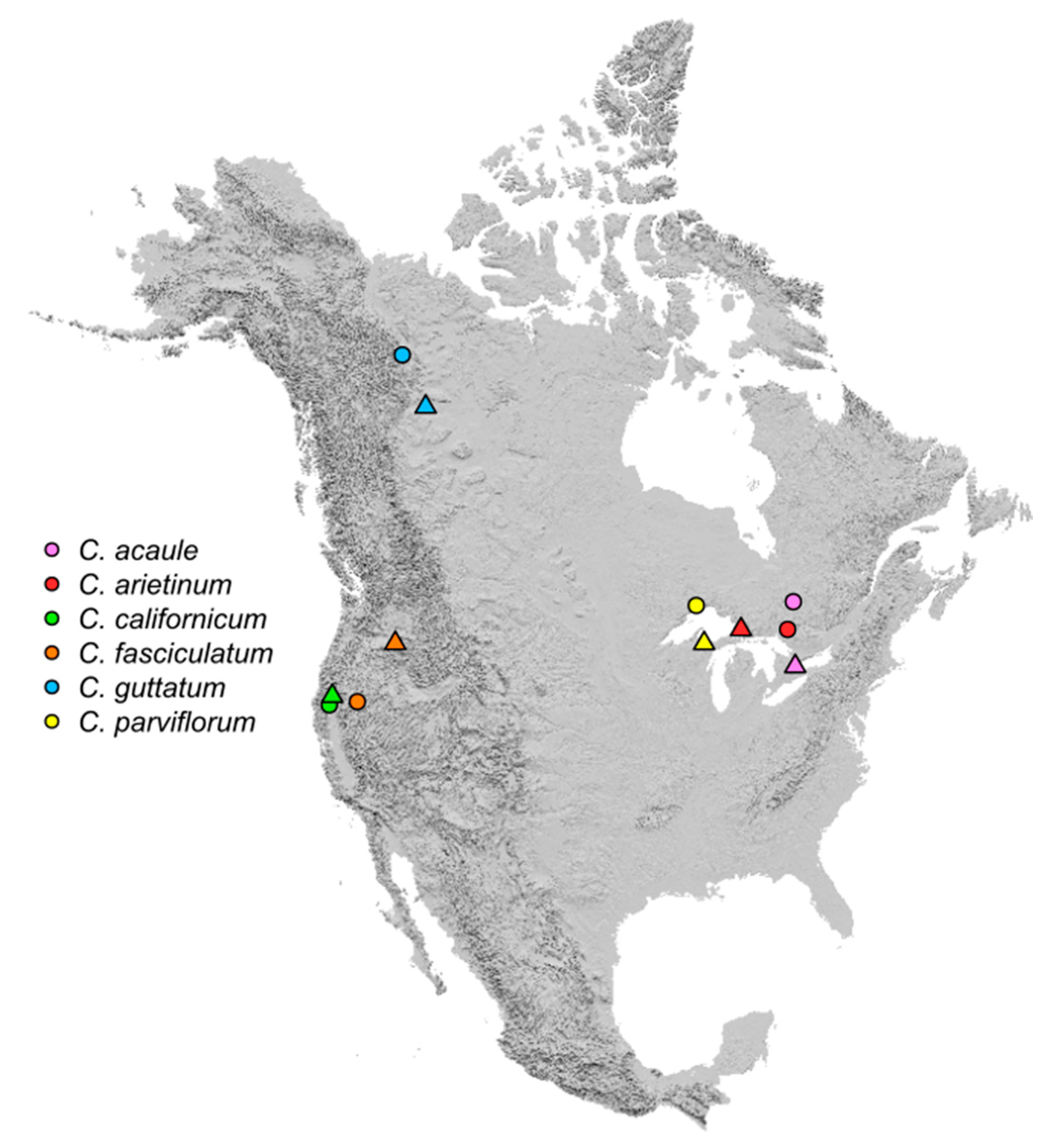
The centroids of suitable habitat shifted by 343.3 km on average (range = 67 to 501 km) and the mean elevational gain across species was 77.3 m (mean %Δ = 16.6%; range = −139 m to 321 m) (Table 1; Figure S1). There was little to moderate overlap in the location of suitable habitat between the two time intervals, with Ω values ranging from 4.2% to 47.4% (mean = 22.9%; Table 1). Models inferred an increase in the total area of habitat for all six Cypripedium spp. between time intervals, with the gains ranging from 564 ha to 156,983 ha. The highest percent change in total area was (%Δ = 2062.2%), inferred for C. fasciculatum. The mean increase in suitable habitat was 82,884 ha (mean %Δ = 528.3%; Table 1). Maxent models reveal increased fragmentation of suitable habitat in the LTI, as quantified by SIP, for C. acaule, C. californicum, C. fasciculatum, and C. parviflorum but reduced fragmentation for C. arietinum and C. guttatum (Table 1).
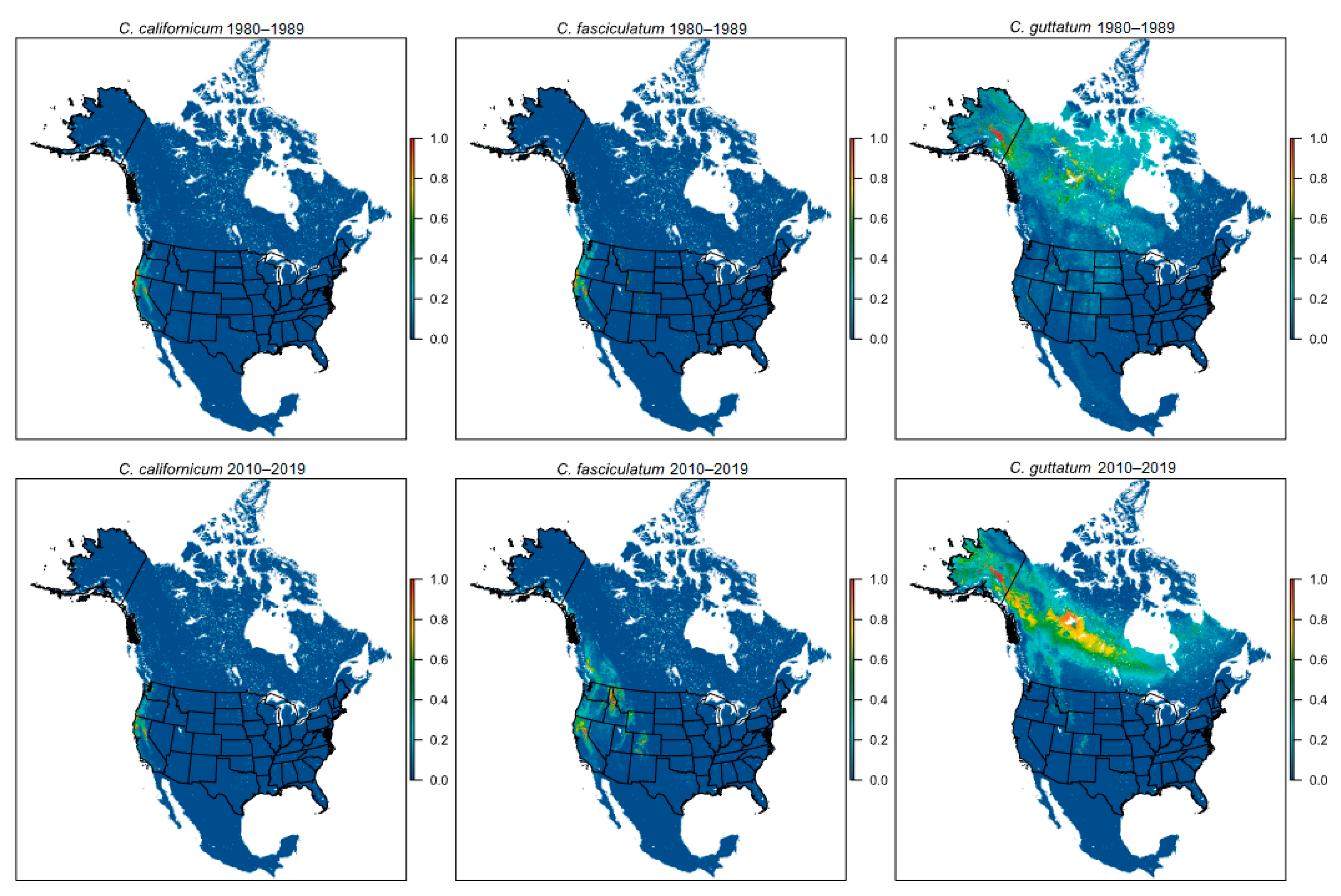
Model inferred centroids of suitable habitat for C. californicum and C. fasciculatum shifted northeastward between the ETI and LTI by 67 km and 501 km, respectively (Figure 1 and Figure S2). While the directionality of habitat shift for these two species was consistent, the change in elevation was not. For C. californium, mean elevation decreased by 139 m (%Δ = −14.7%), while for C. fasciculatum it increased by 321 m (%Δ = 24.8%; Table 1; Figure S1). The area of suitable habitat increased for both species, although the gains differed substantially: C. californicum gained 564 ha (%Δ = 9.1%), while C. fasciculatum gained 79,599 ha (%Δ = 2062.2%; Table 1; Figure 2 and Figure S2). However, for both species suitable habitat became more fragmented with %ΔSIP = 179.2% for C. californicum and 40.1% for C. fasciculatum (Table 1; Figure 2).
The centroid of suitable habitat for C. guttatum shifted to the southeast by 411 km (Figure 1) and mean elevation increased by 84 m (%Δ = 20.1%; Table 1; Figure S1). The extent of suitable habitat increased between time intervals by 104,193 ha (%Δ = 408.0%; Table 1; Figure 2) and models indicate that fragmentation of C. guttatum habitat declined (%ΔSIP = −66.0%).
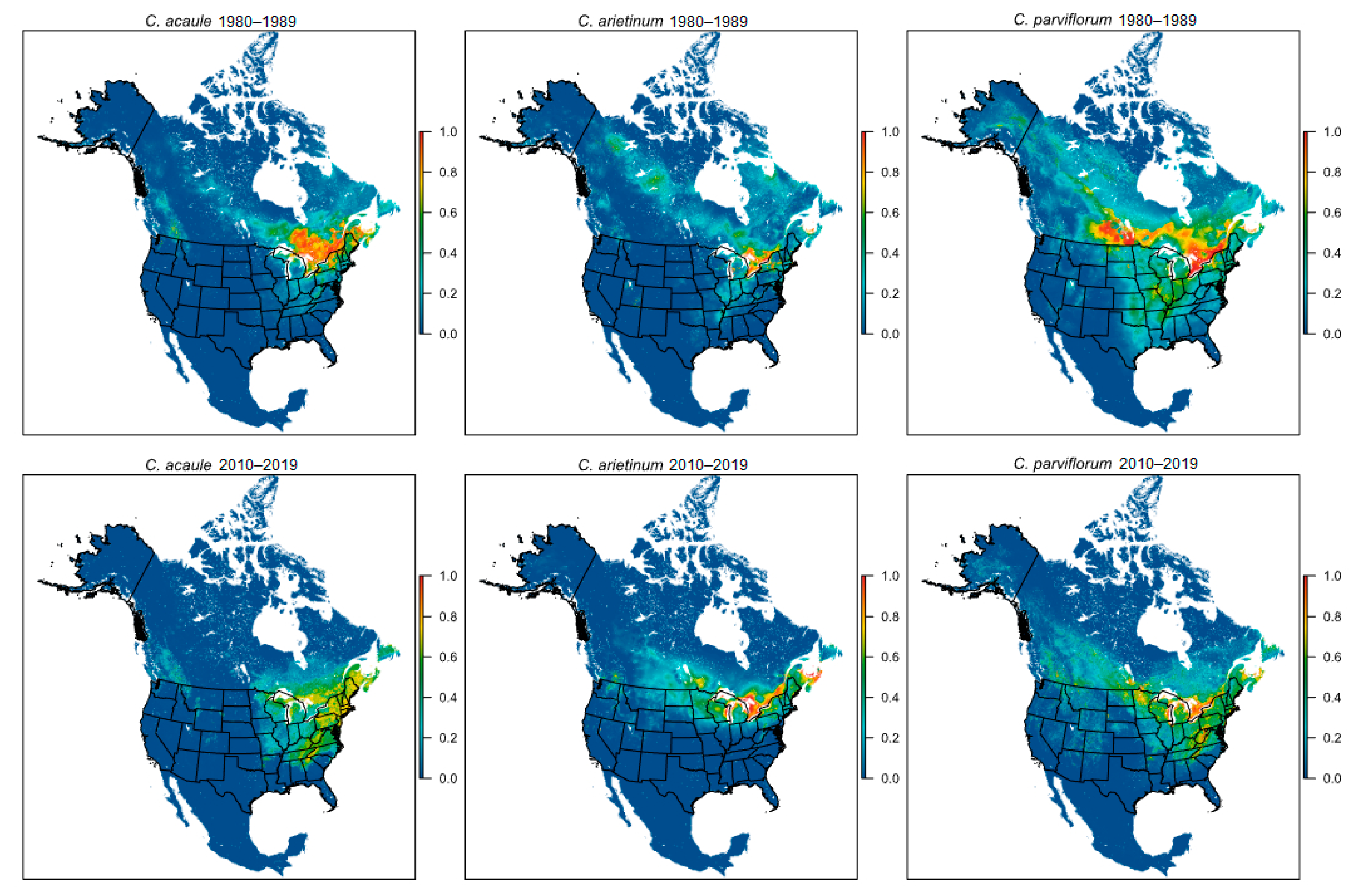
In contrast, the three eastern species did not show a consistent directional response between the ETI and LTI. Models indicate that habitat for C. acaule and C. parviflorum shifted southward (centroid shifts of 466 km and 279 km, respectively), while for C. arietinum it shifted westward (centroid shift of 336 km), with all three species converging on the Great Lakes region (Table 1; Figure 1 and Figure 3 and Figure S3). Mean elevation increased for all three species: 4 m for C. acaule (%Δ = 1.1%), 88 m for C. arietinum (%Δ = 35.8%), and 106 m for C. parviflorum (%Δ = 32.3%; Table 1; Figure S1). Suitable habitat also expanded for all three eastern species by 41,249 ha (C. acaule; %Δ = 26.0%) to 156,983 ha (C. parviflorum; %Δ = 111.2%). However, habitat fragmentation increased for C. acaule (%ΔSIP = 93.7%) and C. parviflorum (%ΔSIP = 83.8%), while it decreased for C. arietinum (%ΔSIP = −81.7%; Table 1).
4. Discussion
Construction and comparison of SDMs for comparable time intervals in the recent past is a powerful approach for objectively assessing shifts in suitable habitat, particularly for rare and/or endangered species. There are also major benefits to including citizen science occurrence records (iNaturalist, NOAH, etc.), not least of which is the wealth of data generated since its advent, as evidenced by the mean increase of 173.1 records per focal Cypripedium species between the ETI, when occurrence data are predominantly from herbarium records, and the LTI when occurrence data are available from both herbarium and citizen science records. A second important advantage is the extensive geographic area potentially surveyed by nature enthusiasts in a given year. One obvious caveat is that citizen science records require close scrutiny and stringent criteria for inclusion in SDMs.
Interestingly, the six North American Cypripedium spp. we investigated showed inconsistent directional shifts of optimal habitat between the two decadal intervals separated by 20 years. However, within the two regions of North America where multiple species occur, there was a more consistent response among species. One interpretation is that species occurring within a region likely have similar environmental requirements. The elevational response between time intervals showed more consistency, with habitat for five of the six species shifting to higher elevations (mean = 77.3 m; Table 1). Only for C. californicum, which requires serpentine soils, did habitat shift to a lower elevation (−139 m). Furthermore, the area of suitable habitat for all six species increased between the ETI and LTI by a mean of 528.3% but habitat became increasingly fragmented for four of the six species.
Cypripediumfasciculatum matched our expectation of a northward shift and elevational increase in optimal habitat between the ETI and LTI, allowing this species to track its climatological niche. While C. californicum also experienced a modest northward shift, it otherwise displayed a distinctly different response. Cypripedium californicum had the highest overlap of optimal habitat between time intervals (Ω = 47.4%), smallest change in total area of suitable habitat (+560 ha), and is the only species with a decline in mean elevation (−139 m). We hypothesize that this response reflects the fact that C. californicum is restricted to serpentine soils, a unique substrate, which is characterized by high metal concentrations, low Ca/Mg ratios, and poor water retention [36,37]. Plants endemic to serpentine soils are more drought resistant than congeners with similar geographic distributions and prior work suggests that these species may be more resilient to a warming climate [62,63,64,65,66,67,68]. However, a plant species’ tolerance does not ensure its long-term viability if essential biotic partners (e.g., pollinators, fungal symbionts) are less resilient to shifts in environmental conditions. While the elevational response of C. californicum appears counter-intuitive, previous work has shown similar elevational responses of co-occurring plant taxa across the mountains surrounding the California central valley, with decreases in water availability at higher elevations in recent decades suggested as the driving mechanism [19].
Cypripedium guttatum experienced a southward shift in suitable habitat and elevational gains. This is likely the only environmental tracking response available to northern species. During the ETI, habitat was located near and within the Arctic Circle with limited available landmass likely hindering a northern shift. Thus, climatic tracking might only be possible for such species by shifting to higher elevations.
More puzzling responses were seen in the three eastern species, for which optimal habitat shifted in different directions, all converging on the area around the Great Lakes. A possible explanation for this is that the moderating influence of large bodies of water to the climate of adjoining land masses slows the rate of warming in the area, thus allowing the Great Lakes region to serve as a refugium. While counter-intuitive, the dramatic southward shift in suitable habitat for C. acaule is not without explanation. Decreasing the productivity of agricultural lands coupled with increasing timber value since the 1940s has resulted in land abandonment and anthropogenic afforestation becoming common across the southeastern United States [69]. Both successional processes and land management for timber production have resulted in the continuous dominance of coniferous forest in recent decades. This has led to an expanded area of ecological conditions that are ideal for C. acaule, which is often restricted to conifer-dominated landscapes.
Suitable habitat for four of the focal Cypripedium species appears to have become more fragmented between the ETI and LTI (Table 1), which appears to be related to shifts to higher elevations on separate mountaintop “islands”. Habitat fragmentation may result in (a) the increased isolation of populations and decreased gene flow among populations, (b) increased genetic drift within populations, and (c) loss of genetic variation and selective potential [70,71,72]. The long-lived habit of Cypripedium spp. may allow for the long-term maintenance of genetic diversity in the absence of gene flow, due to the slowed action of genetic drift, as has been documented for Cypripedium calceolus [30]. Unfortunately, maintaining genetic variation within one generation will not ensure the long-term maintenance of species-wide diversity, nor can it ensure the viability of the plant species if essential biotic partners are adversely impacted by climatic shifts (e.g., decline in pollinators). Fortunately, North American Cypripedium species are typically pollinated by bee species of various genera, due to generalized food mimicry [35,38,39]. This might allow for pollinator switching as the composition of the pollinator community changes in response to climate change.
For the Cypripedium species considered, increased mean elevation of suitable habitat between the ETI and LTI appears to be a more common response than a northward shift. While the expectation is that northward shifts would allow Cypripedium spp. to track climatic conditions, spatial variability in edaphic conditions and the slow rate at which edaphic profiles change could limit range modifications. We found that edaphic conditions strongly influence the distribution of Cypripedium spp. habitat (mean model contribution = 19.2%; Tables S1 and S2); thus, the colonization of habitat that falls within an appropriate climatological envelope may be thwarted by an inhospitable edaphic profile. The distribution of USDA soil orders across North America (Figure S4) indicates that edaphic conditions within a region, regardless of elevation, tend to be highly similar, increasing the likelihood that both climatological and edaphic characteristics are hospitable for Cypripedium spp. at higher elevations nearby. Thus, the colonization of new populations at higher elevations may often be the prevailing response in landscapes with topographic heterogeneity because it requires dispersal over shorter distances and edaphic profiles are more likely to be similar to those of proximate source populations.
The obligate relationship between orchids and their mycorrhizal symbionts may explain the importance of edaphic conditions in delimiting optimal habitat. Orchids are reliant on mycorrhizal associations for the germination and acquisition of soil resources through adulthood [25,42]. It has been shown that edaphic conditions have a stronger influence on fungal distributions than climatic conditions [51]. If suitable habitat for required fungal symbionts is strongly restricted by soil conditions, so too is orchid habitat. The finding of non-climatic environmental variables as strong predictors of suitable habitat suggests that both climatic and non-climatic variables must be considered for more accurate inference of suitable habitat in the past, present, and future. If the distribution of suitable habitat for orchids and their mycorrhizal symbionts becomes decoupled under future climatic conditions, then orchid populations will be unable to persist. Further, the distribution of symbionts must be considered for modeling responses to climate change in species that have an obligate relationship with their symbionts. Unfortunately, studies of the geographic distribution of mycorrhizal symbionts and fungal responses to climate change are almost non-existent and future research into this unexplored topic is much needed.
Our study demonstrates the ability of long-lived perennial plants to respond to recent climatic change through range modification and that responses tend to be regional, suggesting that ecological context may be a better predictor of responses than phylogenetic relatedness. Edaphic conditions are particularly influential in the distribution of these six Cypripedium spp., because of their importance for the occurrence of obligate mycorrhizal symbionts. Thus, range modification of terrestrial orchids in response to a changing climate may only be possible if multiple co-occurring species can respond similarly. However, further work is needed to address questions of how biological assemblages, rather than individual species, might be responding to a changing climate.
Supplementary Materials
The following supporting information can be downloaded at: https://www.mdpi.com/article/10.3390/d14090694/s1, Figure S1: change in mean elevation of suitable habitat; Figure S2: binary suitable habitat for C. californicum, C. fasciculatum, and C. guttatum; Figure S3: binary suitable habitat for C. acaule, C. arietinum, and C. parviflorum; Figure S4: distribution of soil classes across North America; Table S1: bioclimatic correlates of suitable habitat used for SDM construction; Table S2: predictor variables for ETI models; Table S3: predictor variables for LTI models.
Author Contributions
Conceptualization, P.A.S. and D.W.T.; Methodology, P.A.S.; Validation, P.A.S.; Formal Analysis, P.A.S.; Investigation, P.A.S.; Resources, D.W.T.; Data Curation, P.A.S.; Writing—Original Draft Preparation, P.A.S. and D.W.T.; Writing—Review and Editing, P.A.S. and D.W.T.; Visualization, P.A.S. and D.W.T.; Supervision, P.A.S. and D.W.T.; Project Administration, P.A.S. and D.W.T. All authors have read and agreed to the published version of the manuscript.
Funding
This research received no external funding.
Institutional Review Board Statement
Not applicable.
Data Availability Statement
No new data were created or analyzed in this study. Data sharing is not applicable to this article.
Acknowledgments
The authors thank Douda Bensasson, Clayton W. Hale, and J.L. Hamrick for valuable insights that aided in construction of models, as well as three anonymous reviewers.
Conflicts of Interest
The authors declare no conflict of interest.
References
- Roe, G. In defense of Milankovitch. Geophys. Res. Lett. 2006, 33, L24703. [Google Scholar] [CrossRef] [Green Version]
- Eliseev, A.V.; Mokhoc, I.I. Influence of volcanic activity on climate change in the past several centuries: Assessments with a climate model of intermediate complexity. Atmos. Ocean. Phys. 2008, 44, 671–683. [Google Scholar] [CrossRef]
- Montañez, I.P.; McElwain, J.C.; Poilsen, C.J.; White, J.D.; DiMichele, W.A.; Wilson, J.P.; Griggs, G.; Hren, M.T. Climate, , and terrestrial carbon cycle linkages during late Palaeozoic glacial-interglacial cycles. Nat. Geosci. 2016, 9, 824–828. [Google Scholar] [CrossRef]
- PAGES 2k Consortium. Continental-scale temperature variability during the past two millennia. Nat. Geosci. 2013, 6, 339–346. [Google Scholar] [CrossRef]
- Neukom, R.; Steiger, N.; Gómez-Navarro, J.J.; Wang, J.; Wener, J.P. Werner. No evidence for globally coherent warm and cold periods over the preindustrial common era. Nature 2019, 571, 550–554. [Google Scholar] [CrossRef]
- Thornton, P.E.; Thorton, M.M.; Mayer, B.W.; Wei, Y.; Devaralonda, R.; Vose, R.S.; Cook, R.B. Daymet: Daily Surface Weather Data on a 1-km Grid of North America, Version 3; ORNL DAAC: Oak Ridge, TN, USA, 2016. [Google Scholar] [CrossRef]
- Jump, A.S.; Peñuelas, J. Running to stand still: Adaptation and the response of plants to rapid climate change. Ecol. Lett. 2005, 8, 1010–1020. [Google Scholar] [CrossRef]
- Franks, S.J.; Weber, J.J.; Aitken, S.N. Evolutionary and plastic responses to climate change in terrestrial plant populations. Evol. Appl. 2014, 7, 123–139. [Google Scholar] [CrossRef]
- Christmas, M.J.; Breed, M.F.; Lowe, A.J. Constraints to and conservation implications for climate change adaptation in plants. Conserv. Genet. 2016, 17, 305–320. [Google Scholar]
- Hamrick, J.L. Response of forest trees to global environmental changes. For. Ecol. Manag. 2014, 197, 323–335. [Google Scholar] [CrossRef]
- Kremer, A. Long-distance gene flow and adaptation of forest trees to rapid climate change. Ecol. Lett. 2012, 15, 378–392. [Google Scholar] [CrossRef] [Green Version]
- Lenoir, J.; Svenning, J.-C. Climate-related range shifts–a global multidimensional synthesis and new research directions. Ecography 2015, 38, 15–28. [Google Scholar] [CrossRef]
- Steinbauer, M.J. Accelerated increase in plant species richness on mountain summits is linked to warming. Nature 2018, 556, 231–234. [Google Scholar] [CrossRef] [PubMed]
- McGillivray, F.; Hudson, I.L.; Lowe, A.J. Herbarium collections and photographic images: Alternative data sources for phenological research. Biol. Conserv. 2010, 157, 172–177. [Google Scholar]
- Melles, S.J.; Fortin, M.-J.; Lindsay, K.; Badzinski, D. Expanding northward: Influence of climate change, forest connectivity, and population processes on a threatened species’ range shift. Glob. Chang. Biol. 2011, 17, 17–31. [Google Scholar] [CrossRef]
- Robbirt, K.M.; Davy, A.J.; Hutchings, M.J.; Roberts, D.L. Validation of biological collections as a source of phenological data for use in climate change studies: A case study with the orchid Ophrys sphegodes. J. Ecol. 2011, 99, 235–241. [Google Scholar] [CrossRef]
- Hoffmann, A.A.; Rymer, P.D.; Byrne, M.; Ruthrof, K.X.; Whinam, J.; McGeoch, M.; Bergstrom, D.M.; Guerin, G.R.; Sparrow, B.; Joseph, L.; et al. Impacts of recent climate change on terrestrial flora and fauna: Some emerging Australian examples. Austral. Ecol. 2019, 44, 3–27. [Google Scholar] [CrossRef] [Green Version]
- Kelly, A.E.; Goulden, M.L. Goulden. Rapid shifts in plant distribution with recent climate change. Proc. Natl. Acad. Sci. USA 2008, 105, 11823–11826. [Google Scholar] [CrossRef] [Green Version]
- Crimmins, S.M.; Dobrowski, S.Z.; Greenberg, J.A.; Abatzoglou, J.T.; Mynsberge, A.R. Changes in climatic water balance drive downhill shifts in plant species’ optimum elevations. Science 2011, 331, 258–261. [Google Scholar] [CrossRef]
- Bertrand, R.; Lenoir, J.; Piedallu, C.; Riofrío-Dillon, G.; de Ruffray, P.; Vidal, C.; Pierrat, J.-C.; Gégout, J.-C. Changes in plant community composition lag behind climate warming in lowland forest. Nature 2011, 479, 517–520. [Google Scholar] [CrossRef]
- Nicholé, F.; Brzosko, E.; Till-Bottraud, I. Population viability analysis of Cypripedium calceolus in a protected area: Longevity, stability and persistence. J. Ecol. 2005, 93, 716–726. [Google Scholar] [CrossRef]
- Dressler, R.L. The Orchids: Natural History and Classification; England Harvard University Press: Cambridge, MA, USA, 1981. [Google Scholar]
- Rasmussen, H. Terrestrial Orchids: From Seed to Mycotrophic Plant; Cambridge University Press: New York, NY, USA, 1995. [Google Scholar]
- Arditti, J.; Ghani, K.A. Tansley review no. 110: Numerical and physical properties of orchid seeds and their biological implications. New Phytol. 2000, 145, 367–421. [Google Scholar] [CrossRef] [Green Version]
- Cozzolino, S.; Cafasso, D.; Pellegrino, G.; Musacchio, A.; Widmer, A. Fine-scale phylogeographical analysis of Mediterranean Anacamptis palustris (Orchidaceae) populations based on chloroplast minisatellite and microsatellite variation. Mol. Ecol. 2003, 12, 2783–2792. [Google Scholar] [CrossRef]
- Trapnell, D.W.; Hamrick, J.L. Partitioning nuclear and chloroplast variation at multiple spatial scales in the Neotropical epiphytic orchid, Laelia rubescens. Mol. Ecol. 2004, 13, 2655–2666. [Google Scholar] [CrossRef]
- Hamrick, J.L.; Trapnell, D.W. Using population genetic analyses to understand patterns of seed dispersal. Acta Oecol. 2011, 37, 641649. [Google Scholar] [CrossRef]
- Kartzinel, T.R.; Shefferson, R.P.; Trapnell, D.W. Relative importance of pollen and seed dispersal across a Neotropical mountain landscape for an epiphytic orchid. Mol. Ecol. 2013, 22, 6048–6059. [Google Scholar] [CrossRef]
- Broeck, A.V.; Landuyt, W.V.; Cox, K.; Bruyn, L.D.; Gyselings, R.; Oostermeijer, G.; Valentin, B.; Bozic, G.; Dolinar, B.; Illyés, Z.; et al. High levels of effective long-distance dispersal may blur ecotypic divergence in a rare terrestrial orchid. BMC Ecol. 2014, 14, 20. [Google Scholar]
- Minasiewicz, J.; Znaniecka, J.M.; Górniak, M.; Kawiński, A. Spatial genetic structure of an endangered orchid Cypripedium calceolus (Orhcidaceae) at a regional scale: Limited gene flow in a fragmented landscape. Conserv. Genet. 2018, 19, 1149–1460. [Google Scholar] [CrossRef] [Green Version]
- Trapnell, D.W.; Hamrick, J.L.; Smallwood, P.A.; Kartzinel, T.R.; Ishibashi, C.D.; Quigley, C.T.C. Phylogeography of the Neotropical epiphytic orchid, Brassavola nodosa: Evidence for a secondary contact zone in northwestern Costa Rica. Heredity 2019, 123, 662–674. [Google Scholar] [CrossRef]
- Kotilínek, M.; Tĕšitelová, T.; Košnar, J.; Fibich, P.; Hemrová, L.; Koutecký, P.; Münzber-gová, Z.; Jersáková, J. Seed dispersal and realized gene flow of two forest orchids in a fragmented landscape. Plant Biol. 2020, 22, 522–532. [Google Scholar] [CrossRef]
- Trapnell, D.W.; Hamrick, J.L.; Ishibashi, C.D.; Kartzinel, T.R. Genetic inference of epiphytic orchid colonization; it may only take one. Mol. Ecol. 2013, 22, 3680–3692. [Google Scholar] [CrossRef]
- The IUCN Red List of Threatened Species, Version 2020-1; IUCN: Grand, Switzerland, 2020; Available online: https://www.iucnredlilst.org (accessed on 3 August 2021).
- Cribb, P. The Genus Cypripedium; Timber Press: Portland, OR, USA, 1997. [Google Scholar]
- Alexander, E.B.; Coleman, R.G.; Keeler-Wolf, T.; Harrison, S.P. Serpentine Geoecology of Western North America: Geology, Soils, and Vegetation; Oxford University Press: New York, NY, USA, 2007. [Google Scholar]
- Coleman, R.A. The Cypripedium of the United States and Canada. Part III: Arietinum, californicum, fasciculatum, guttatum, yatabeanum and X alaskanum. Orchids 2018, 87, 522–529. [Google Scholar]
- Stoutamire, W.P. Flower biology of the Lady’s-slippers (Orchidaceae: Cypripedium). Mich. Bot. 1967, 6, 159–175. [Google Scholar]
- Argue, C.L. The Pollination of North American Orchids: Volume 1: North of Florida and Mexico; Springer: New York, NY, USA, 2012. [Google Scholar]
- Withner, C.L. The Orchids: A Scientific Survey; The Ronald Press Co.: New York, NY, USA, 1959. [Google Scholar]
- Shefferson, R.P.; Bunch, W.; Cowden, C.C.; Lee, Y.-I.; Kartzinel, T.R.; Yukawa, T.; Downing, J.; Jiang, H. Does evolutionary history determine specificity in broad ecological interactions? J. Ecol. 2019, 107, 1582–1593. [Google Scholar] [CrossRef]
- Smith, S.E.; Read, D.J. Mycorrhizal Symbiosis, 3rd ed.; Academic Press: New York, NY, USA, 2010. [Google Scholar]
- Shefferson, R.P.; Jacquemyn, H.; Kull, T.; Hutchings, M.J. The demography of terrestrial orchid: Life history, population dynamics and conservation. Bot. J. Linn. Soc. 2020, 192, 315–332. [Google Scholar] [CrossRef]
- Shefferson, R.P.; Warren, I.I.; Pulliam, H.R. Life history costs make perfect sprouting maladaptive in two herbaceous perennials. J. Ecol. 2014, 102, 1318–1328. [Google Scholar] [CrossRef] [Green Version]
- Phillips, S.J.; Anderson, R.P.; Dudík, M.; Schapire, R.E.; Blair, M.E. Opening the black box: An open-source release of Maxent. Ecography 2017, 40, 887–893. [Google Scholar] [CrossRef]
- GBIF.org GBIF Occurrence Download. 2018. Available online: https://doi.org/10.15468/dl.dujw5l (accessed on 2 February 2020).
- Pebesma, E.J.; Bivand, R.S. 2005. Classes and Methods for Spatial Data in R-R News 5: 2. Available online: https://cran.r-project.org/doc/Rnews (accessed on 20 September 2018).
- R: A language and environment for statistical computing. In R Foundation for Statistical Computing; R Core Team: Vienna, Austria, 2020; Available online: https://www.R-project.org (accessed on 17 September 2018).
- Hijman, R.J.; Phillips, S.; Leathwick, J.; Elith, J. Dismo: Species Distribution Modeling, R Package Version 1.1-4; 2017. Available online: https://CRAN.R-project.org/package=dismo (accessed on 5 August 2018).
- Hengl, T.; de Jesus, J.M.; Heuvelink, G.B.M.; Gonzalez, M.R.; Kilibarda, M.; Blagotić, A.; Shangguan, W.; Wright, M.N.; Geng, X.; Bauer-Marscallinger, B.; et al. SoilGrids250m: Global gridded soil information based on machine learning. PLoS ONE 2017, 12, e0169748. [Google Scholar] [CrossRef] [Green Version]
- Tedersoo, L.; Bahram, M.; Põlme, S.; Kõljalg, U.; Yorou, N.S.; Wijesundera, R.; Ruiz, L.V.; Vasco-Palacios, A.M.; Thu, P.Q.; Siuja, A.; et al. Global diversity and geography of soil fungi. Science 2014, 346, 1256688. [Google Scholar] [CrossRef] [Green Version]
- ESA. Land Cover CCI Produce User Guider Version 2. Tech. Rep. 2017. Available online: Maps.elie.ucl.ac.be/CCI/viewer/download/ESACCI-LC-Ph2-PUGv2_2.0.pdf (accessed on 1 April 2022).
- Fielding, A.H.; Bell, J.F. A review of methods for the assessment of prediction errors in conservation presence/absence models. Environ. Conserv. 1997, 24, 38–49. [Google Scholar] [CrossRef]
- Clifford, P.; Richardson, S.; Hermon, D. Assessing the significance of the correlation between two spatial processes. Biometrics 1989, 45, 123–134. [Google Scholar] [CrossRef]
- Dutilleul, P. Modifying the t test for assessing the correlation between two spatial processes. Biometrics 1993, 49, 305–314. [Google Scholar] [CrossRef]
- Vallejos, R.; Osorio, F.; Bevilacqua, M. Spatial Relationships between Two Georeferenced Variables: With Applications in R.; Springer: New York, NY, USA, 2020. [Google Scholar]
- Liu, C.; Newell, G.; White, M. On the selection of thresholds for predicting species occurrence with presence-only data. Ecol. Evol. 2016, 6, 337–348. [Google Scholar] [CrossRef] [Green Version]
- Kou, X.; Li, Q.; Liu, S. Quantifying species’ range shifts in relation to climate change: A case study of Abies spp. in China. PLoS ONE 2011, 6, e23115. [Google Scholar] [CrossRef]
- Amante, C.; Eakins, B.W. ETOPO1 Arc-Minute Global Relief Model: Procedures, Data Sources and Analysis; NOAA: Washington, DC, USA, 2009. [Google Scholar]
- Patton, D.R. A diversity index for quantifying habitat “edge”. Wildl. Soc. Bull. 1975, 3, 171–173. [Google Scholar]
- Forman, R.T.T.; Godron, M. Landscape Ecology; John Wiley and Sons: New York, NY, USA, 1986. [Google Scholar]
- Cooke, S.S. The Edaphic Ecology of Two Western North American Composite Species. Ph.D. Thesis, University of Washington, Seattle, WA, USA, 18 August 1994. [Google Scholar]
- Armstrong, J.K.; Huenneke, L.F. Spatial and temporal variation in species composition in California grasslands: The interaction of drought and substratum. In The Vegetation of Ultramafic (Serpentine) Soils; Baker, A.J.M., Proctor, J., Reeves, R.D., Eds.; Andover: Hampshire, UK, 1992; pp. 213–233. [Google Scholar]
- Grime, J.P.; Brown, V.K.; Thompson, K.; Masters, G.J.; Hiller, S.H.; Clarke, I.P.; Askew, A.P.; Corker, D.; Kielty, J.P. The response of two contrasting limestone grasslands to simulated climate change. Science 2000, 289, 762–765. [Google Scholar] [CrossRef]
- Grime, J.P.; Fridley, J.D.; Askew, A.P.; Thompson, K.; Hodgson, J.G.; Bennett, C.R. Long-term resistance to simulated climate change in an infertile grassland. Proc. Natl. Acad. Sci. USA 2008, 105, 10028–10032. [Google Scholar] [CrossRef] [Green Version]
- Hughes, R.; Konrad, B.; Smirnoff, N.; Macnair, M.R. The role of drought tolerance in serpentine tolerance in the Mimulus guttatus Fisher ex DC. complex. S. Afr. J. Sci. 2001, 97, 581–586. [Google Scholar]
- Damschen, E.I.; Harrison, S.; Ackerly, D.D.; Fernandez-Going, B.M.; Anacker, B.L. Endemic plant communities on special soils: Early victims or hardy survivors of climate change? J. Ecol. 2012, 100, 1122–1130. [Google Scholar] [CrossRef]
- Fernandez-Going, B.M.; Anacker, B.L.; Harrison, S.P. Temporal variability in California grasslands: Soil type and species functional traits mediate response to precipitation. Ecology 2012, 93, 2104–2114. [Google Scholar] [CrossRef]
- Wear, D.N. Land use. In Southern Forest Resource Assessment. General Technical Report; Wear, D.N., Greis, J.G., Eds.; USDA, Forest Service: Washington, DC, USA, 2002; pp. 153–174. [Google Scholar]
- Young, A.; Boyle, T.; Brown, T. The population genetic consequences of habitat fragmentation for plants. Trends Ecol. Evol. 1996, 11, 413–418. [Google Scholar] [CrossRef]
- Laurance, W.F.; Lovejoy, T.E.; Vasconcelos, H.L.; Bruna, E.M.; Didham, R.K.; Stouffer, P.C.; Gascon, C.; Bierregaard, R.O.; Laurance, S.G.; Sampaio, E. Ecosystem decay of Amazonian forest fragments: A 22-year investigation. Conserv. Biol. 2002, 16, 605–618. [Google Scholar] [CrossRef] [Green Version]
- Reed, D.H. Extinction risk in fragmented habitat. Anim. Conserv. 2004, 7, 181–191. [Google Scholar] [CrossRef]
Figure 1.
Map showing directional shifts of suitable habitat centroids for six Cypripedium species in North America between the ETI and LTI. Colors represent species, circles represent ETI centroids, and triangles represent LTI centroids.
Figure 1.
Map showing directional shifts of suitable habitat centroids for six Cypripedium species in North America between the ETI and LTI. Colors represent species, circles represent ETI centroids, and triangles represent LTI centroids.

Figure 2.
Maps showing Maxent cloglog predictions of suitable habitat for the three western species: C. californicum, C. fasciculatum, and C. guttatum. The top row illustrates the ETI prediction and the bottom row shows the LTI model. Colors illustrate suitability of habitat, with red indicating optimal habitat and dark blue indicating the least suitable habitat.

Figure 3.
Maps showing Maxent cloglog prediction of suitable habitat for the three eastern species: C. acaule, C. arietinum, and C. parviflorum. The top row illustrates the ETI prediction and the bottom the LTI. Colors illustrate suitability of habitat, with red indicating optimal habitat and dark blue indicating the least suitable habitat.


Table 1.
Summary statistics from species distribution models for six North American Cypripedium species for the early (ETI; 1980 to 1989) and late time intervals (LTI; 2010 to 2019). Measures include the number of occurrence records included in model construction (N), percent of records correctly predicted (PCC), overlap criterion (Ω), change in total area of suitable habitat between time intervals (Δ area), percent change in total area (%Δ area), distance the centroid of suitable habitat shifted, change in mean elevation of suitable habitat (Δ elevation), percent change in mean elevation (%Δ elevation), and percent change in Patton’s shape index (%Δ SIP), which is an estimate of change in degree of habitat fragmentation.
| Species | N (ETI) | N (LTI) | PCC (ETI) | PCC (LTI) | Ω | Δ Area (ha) | %Δ Area | Centroid Shift (km) | Δ Elevation (m) | %Δ Elevation | %Δ SIP |
|---|---|---|---|---|---|---|---|---|---|---|---|
| West | |||||||||||
| C. californicum | 35 | 78 | 71.4% | 92.3% | 47.4% | 564 | 9.1% | 67 | −139 | −14.7% | 179.2% |
| C. fasciculatum | 17 | 53 | 64.7% | 94.3% | 4.2% | 79,599 | 2062.2% | 501 | 321 | 24.8% | 40.1% |
| C. guttatum | 12 | 34 | 91.7% | 82.4% | 10.7% | 104,193 | 408.0% | 411 | 84 | 20.1% | −66.0% |
| Mean | 21.3 | 55.0 | 75.93% | 89.67% | 20.77% | 61,452.0 | 826.43% | 326.3 | 88.6 | 10.07% | 51.10% |
| East | |||||||||||
| C. acaule | 82 | 4654 | 81.7% | 97.2% | 39.7% | 41,249 | 26.0% | 466 | 4 | 1.1% | 93.7% |
| C. arietinum | 11 | 91 | 72.7% | 93.4% | 11.5% | 114,714 | 553.5% | 336 | 88 | 35.8% | −81.7% |
| C. parviflorum | 81 | 1560 | 67.9% | 92.7% | 23.9% | 156,983 | 111.2% | 279 | 106 | 32.3% | 83.8% |
| Mean | 58.0 | 2101.7 | 74.10% | 94.43% | 25.03% | 104,315.3 | 230.23% | 360.3 | 66.0 | 23.07% | 31.93% |
| Overall mean | 39.7 | 1078.4 | 75.02% | 92.05% | 22.90% | 82,883.7 | 528.33% | 343.3 | 77.3 | 16.57% | 41.52% |
Publisher’s Note: MDPI stays neutral with regard to jurisdictional claims in published maps and institutional affiliations. |
© 2022 by the authors. Licensee MDPI, Basel, Switzerland. This article is an open access article distributed under the terms and conditions of the Creative Commons Attribution (CC BY) license (https://creativecommons.org/licenses/by/4.0/).
Share and Cite
MDPI and ACS Style
Smallwood, P.A.; Trapnell, D.W. Species Distribution Modeling Reveals Recent Shifts in Suitable Habitat for Six North American Cypripedium spp. (Orchidaceae). Diversity 2022, 14, 694. https://doi.org/10.3390/d14090694
AMA Style
Smallwood PA, Trapnell DW. Species Distribution Modeling Reveals Recent Shifts in Suitable Habitat for Six North American Cypripedium spp. (Orchidaceae). Diversity. 2022; 14(9):694. https://doi.org/10.3390/d14090694
Chicago/Turabian StyleSmallwood, Patrick A., and Dorset W. Trapnell. 2022. "Species Distribution Modeling Reveals Recent Shifts in Suitable Habitat for Six North American Cypripedium spp. (Orchidaceae)" Diversity 14, no. 9: 694. https://doi.org/10.3390/d14090694
Note that from the first issue of 2016, this journal uses article numbers instead of page numbers. See further details here.