Article

High-Resolution Mapping of Seagrass Biomass Dynamics Suggests Differential Response of Seagrasses to Fluctuating Environments

Department of Life Sciences and Innovation and Development Center of Sustainable Agriculture, National Chung Hsing University, Taichung 40227, Taiwan
*
Author to whom correspondence should be addressed.
Diversity 2022, 14(11), 999; https://doi.org/10.3390/d14110999
Submission received: 1 October 2022 / Revised: 12 November 2022 / Accepted: 16 November 2022 / Published: 19 November 2022
(This article belongs to the Special Issue Ecology, Diversity and Conservation of Seagrass)

Abstract

:
Seagrass beds are major blue carbon ecosystems. Climate change-associated factors may change the seagrass community and affect the capacity of carbon sequestration. To explore the possible effects of warming, higher precipitation levels and/or sea level rise on seagrasses, the spatial and seasonal dynamics in shallow seagrass beds comprising the late-successional seagrass Thalassia hemprichii and the early-successional seagrass Halodule uninervis were tracked. The high-resolution mapping of seagrass biomass dynamics showed that T. hemprichii was the dominant species in the study sites year round, as the space occupation by the larger seagrass T. hemprichii was more efficient than that by the smaller seagrass H. uninervis. The space occupation by both species in the low-elevation site was more efficient than in the high-elevation site. In the low-elevation site, while the dominance of the faster growing seagrass H. uninervis was increasing, the dominance of T. hemprichii was decreasing. This suggested that the carbon sequestration capacity of the seagrass beds will decrease, as T. hemprichii was capable of storing more carbon in the sediments. In the high-elevation site, however, the distribution of both species was distinct and showed a clear seasonal succession. The dominance of H. uninervis moved to shallower water in the wet season and then moved back to deeper water in the dry season. Our observations suggested that four possible mechanisms might be involved in the dominance shift in the shallow seagrass beds: (1) the deeper water in the low-elevation site or the higher precipitation levels in the wet season might reduce the drought stress of H. uninervis at low tide and enhance the competition of H. uninervis over T. hemprichii; (2) the growth of H. uninervis might be stimulated more by the flushing of land-based nutrients caused by the higher precipitation rates in the wet season; (3) in the high-elevation site, the faster flow velocity and frequently disturbed sediments in the dry season might constrain the further expansion of H. uninervis to shallower water; (4) the faster flow velocity in the high-elevation site might reduce the impacts of periphyton overgrowth on T. hemprichii and maintain the dominance of T. hemprichii in the community. Our results suggest seagrasses will not necessarily respond to fluctuating environments in the same way in the coming decades.

1. Introduction

Blue carbon ecosystems such as seagrass beds, mangroves and salt marshes can sequester large quantities of carbon efficiently and effectively in the sediments [1,2]. Among these ecosystems, the global area of seagrass beds (0.788 × 10⁶ km2) is 4 times the sum of mangroves and salt marshes (0.194 × 10⁶ km2) [3]. The contribution to global net primary production by seagrasses (310–353 Tg C yr−1) is 2 to 4 times the sum of mangroves (54–138 Tg C yr−1) and salt marshes (24–60 Tg C yr−1) [4]. It is clear that seagrass beds function as critical carbon sinks so that any change in the community may affect the carbon sequestration capacity and coastal carbon cycle.
The carbon sequestration capacity of seagrass beds may vary with seagrass species within the community. In the Indo-Pacific region, Thalassia hemprichii and Halodule uninervis are the dominant seagrasses in shallow waters [5]. T. hemprichii is considered the late-successional seagrass dominating the intertidal zone, whereas H. uninervis is the early-successional species occupying the subtidal zone [6]. For both species, most of the leaf production decomposes within a year [7]. However, the turnover rates of the belowground portion are much longer than those of the aboveground portion. Up to 53% of the long-term organic carbon burial in the sediments might be derived from belowground production [8]. Due to the lower turnover and slower decomposition rates of the belowground portion, T. hemprichii (2.57 ± 0.32 g C m−2 yr−1) can store more carbon in the sediments than H. uninervis (1.49 ± 0.43 g C m−2 yr−1) [8].
Anthropogenic combustion of fossil fuels and land use changes over the past two centuries have fundamentally altered the global carbon cycle [9]. The global average of carbon dioxide (CO2) bypassed 418 ppm in April 2022 (https://www.esrl.noaa.gov/gmd/ccgg/trends/global.html, accessed on 17 July 2022). Compared to 1850–1900, the global surface temperature will increase by 1.0–1.8 °C under SSP1–1.9 and by 3.3–5.7 °C under SSP5–8.5 by 2081–2100 [10]. It is very likely that heavy precipitation events will intensify and become more frequent in most regions with additional global warming. Relative to 1995–2014, the global sea level will rise 0.28–0.55 m (SSP1–1.9) to 0.63–1.01 m (SSP5–8.5) by 2100 [10]. These climate change-associated factors are expected to affect the distribution or physiology of seagrass species [11]. Global warming may cause the migration of temperate seagrasses to higher latitude regions [12]. The greater frequency and higher intensity of heat waves may cause damage to seagrass beds [13] and declines in seagrass biomass and productivity [14,15]. Sea level rise will reduce the exposure time of intertidal seagrasses, which may cause the migration of less drought-resistant species such as H. uninervis landward, and thus increase the carbon sinks [16]. However, the resulting deep water may reduce the received irradiance of subtidal seagrasses and the carbon sequestration capacity [17]. Sea level rise may also induce wave disturbance in shallow waters, which may resuspend sediments and cause unstable sediments for seagrass colonization [18]. Ocean acidification and warming may lead to increases in the belowground biomass and carbon sequestration of T. hemprichii [19]. Wind speed and rainfall are most responsible for the seasonal variations in the abundance and growth of T. hemprichii in southern Taiwan [20]. T. hemprichii is vulnerable to the higher precipitation levels of La Niña events due to the flushing of land-based nutrients into the sea and the overgrowth of periphyton [6].
Seagrass beds are not only important blue carbon sinks but also crucial habitats and feeding grounds for consumers [21]. It will be important to document how blue carbon ecosystems and the carbon sequestration capacity are impacted by climate change-associated factors [10]. In this study, the possible response of T. hemprichii and H. uninervis to either warming, higher precipitation and/or sea level rise were assessed by tracking the seasonal and spatial succession of both species across seasons in high- and low-elevation sites. It was hypothesized that both T. hemprichii and H. uninervis would respond positively to warming and higher precipitation in the wet season. Deeper water in the low-elevation site or higher precipitation in the wet season was hypothesized to reduce the drought stress of H. uninervis and increase the dominance in the community due to the competition for space.

2. Materials and Methods
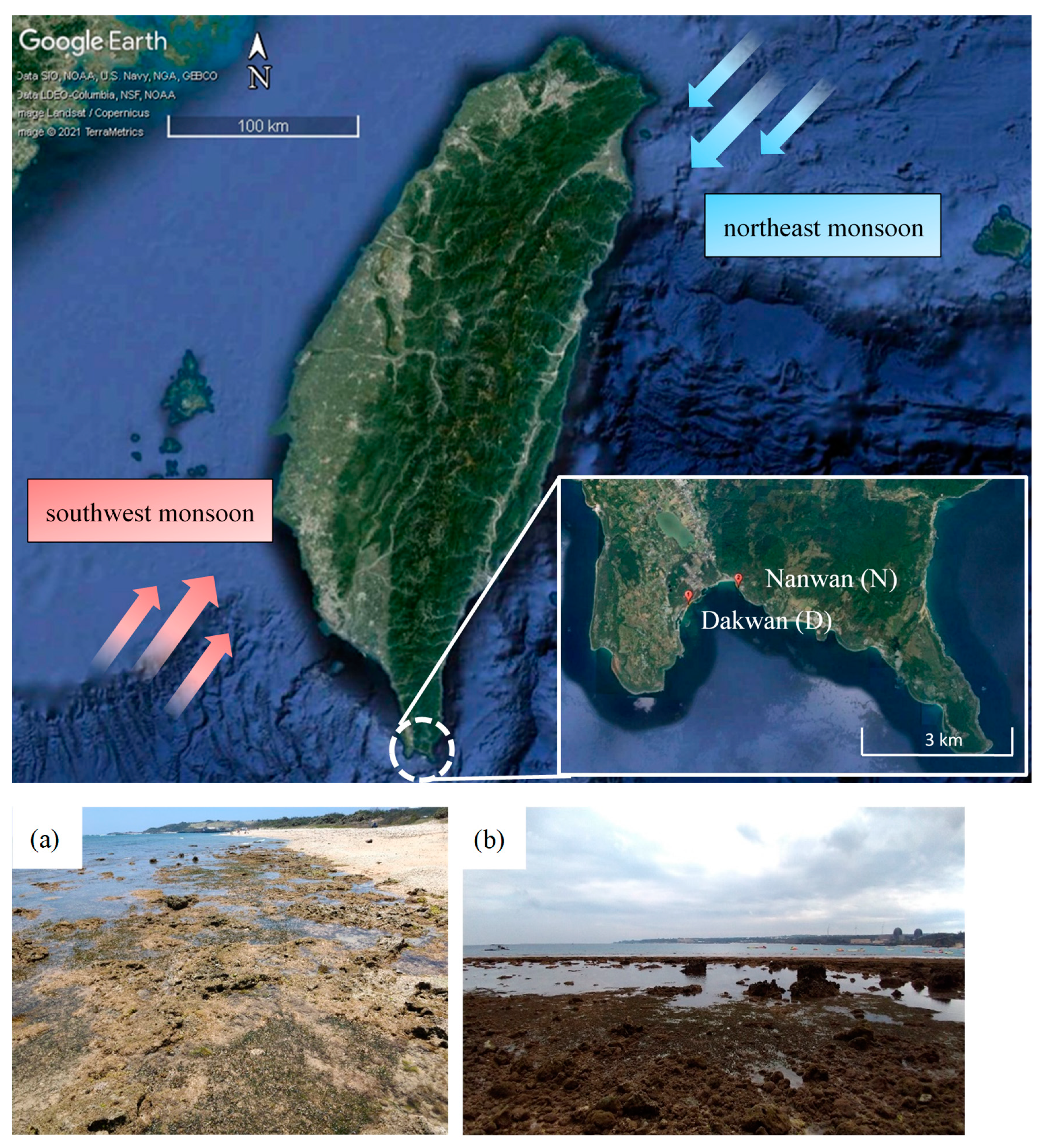
2.1. Study Sites

There were two study sites, the high-elevation site Dakwan (21.95038, 120.74888) and the low-elevation site Nanwan (21.95646, 120.76826), located in the intertidal fringing reef platforms of Nanwan Bay, southern Taiwan (Figure 1). The air temperature was higher in summer (mean: 28.7 °C) and lower in winter (mean: 22.1 °C) (https://e-service.cwb.gov.tw/HistoryDataQuery/ accessed 11 July 2022). Monthly precipitation was also higher in summer (548 mm) and lower in winter (42 mm). The wind speed was faster in winter (mean: 5.5 m/s) during the northeast monsoon and slower in summer during the southwest monsoon (mean: 2.0 m/s).
The areas of seagrass beds in Dakwan and Nanwan were 1800 m2 and 400 m2, respectively. T. hemprichii and H. uninervis were the only two seagrass species mixed in the seagrass beds. The coast of Nanwan Bay had a mixed and predominantly semidiurnal tidal cycle (Chinese Naval Hydrographic and Oceanographic Office). The tidal range along the coast was 1–2 m. The relative substrate elevation was relative to the local chart datum based on the mean sea level of the tide gauge station in Nanwan. Dakwan and Nanwan were −52 and −64 cm above the chart datum, respectively. During spring low tides, the exposure time of seagrasses in Dakwan (high-elevation site) was 4 h, whereas seagrasses in Nanwan (low-elevation site) were exposed to the air for ephemeral periods (minutes–hours).
At each site, there was a fixed transect line perpendicular to the shore. The length of the transect at each site (Dakwan 27 m, Nanwan 21 m) depended on the width of the seagrass bed and extended to the outer limits of the bed. Environmental and seagrass data were acquired within 2 h during low tides along the transect lines in January (winter), April (spring), July (summer), and October (autumn) from April 2018 to April 2020. According to the monthly precipitation data (https://e-service.cwb.gov.tw/HistoryDataQuery/ accessed 11 July 2022), the data collected in winter and spring were classified as the dry season, and the data collected in summer and autumn were classified as the wet season for analyses of the relationship between the seagrass variables and environmental factors, which can be used to explore the possible mechanisms involved in the seagrass dynamics.

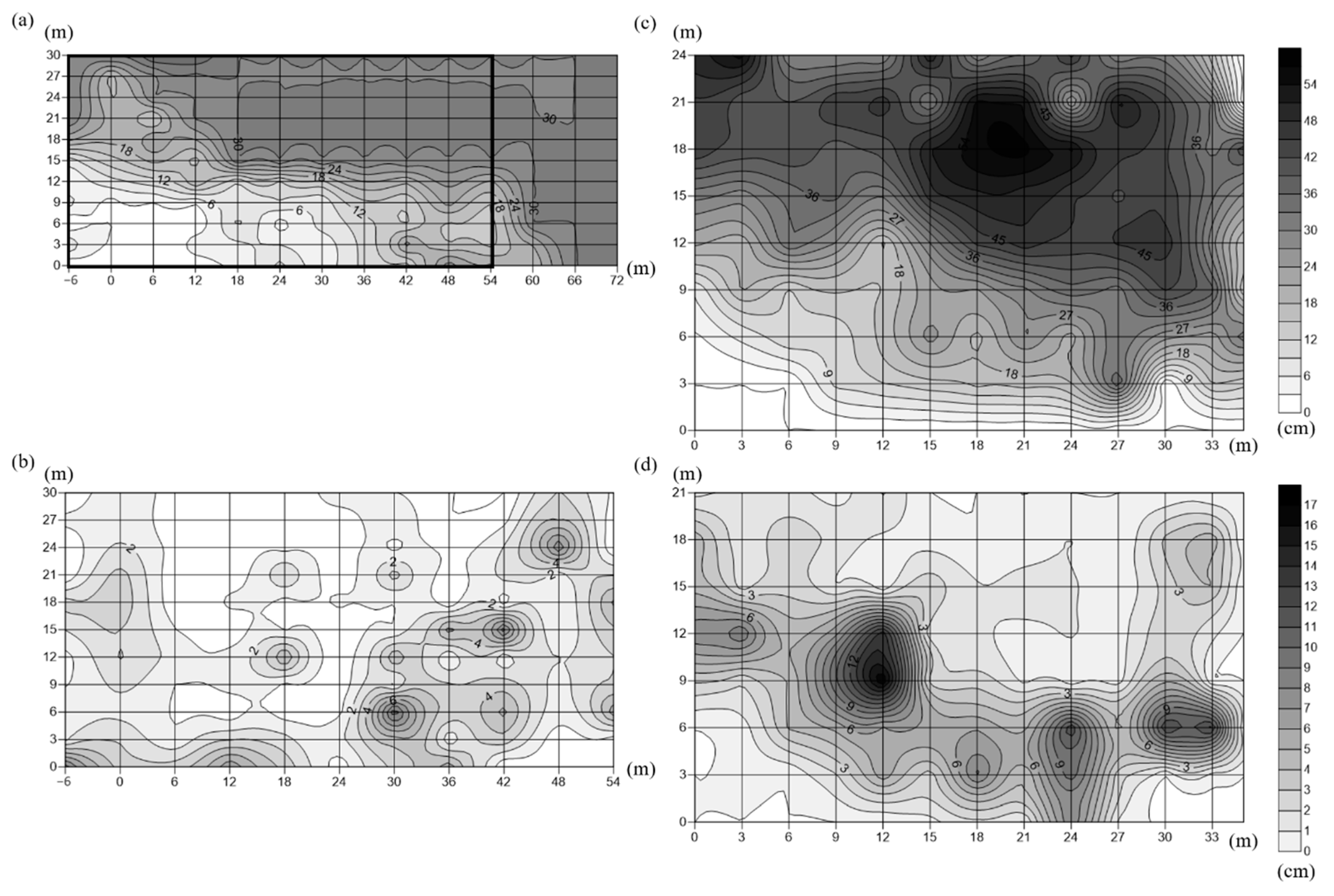
2.2. Sediment Features and Water Quality

Sediment depth was determined by vertically forcing an iron nail (approximately 30 cm) into the sediments until the top of the nail reached a solid substrate of coral reefs at five randomly selected locations at each site for each sampling time [8]. Two of the five measurements were further verified to determine whether the top of the nail reached the bottom of the sediments at each site for each time. Sediment samples were collected at three randomly selected locations near but not directly along the transect line of each site for each time. Cores of the top 5 cm were extracted using a 3.5 cm diameter PVC corer. The sediments were passed through a 0.5 mm sieve to remove large plant and animal pieces. The grain size, silt/clay (S/C) content and sorting coefficient of the sediments were determined following the granulometry methods [22].
Seawater temperature, salinity, turbidity, depth and DIN (NH4+ + NO2 + NO3) and DIP (PO43−) concentrations were also measured in five replicates at each site for each time at low tide. Temperature and salinity were measured using a portable YSI-600XLM meter (YSI, Yellow Springs, OH, USA). Turbidity, defined as the water extinction coefficient for photosynthetically active radiation (PAR), was determined by light measurements using a Li-Cor Li-189 quantum meter. Water depth was measured with a ruler. Water samples collected for the nutrient analysis were filtered in the field through 0.45 μm MFS cellulose nitrate membrane filters and transported back to the laboratory on ice. In the laboratory, these samples were analyzed colorimetrically for PO43− [23], NH4+ [24], NO3 [25] and NO2 [26] concentrations.
The weight loss of the Plaster of Paris as a quantitative expression of the water motion over a period of time was used to measure the hydrography in the shallow seagrass beds [27]. The relative flow velocity at each site in each season was determined using the weight loss of the Plaster of Paris (approximately 36 g dry weight, n = 6) after 1 day of submersion in the water following the procedure [28].

2.3. Seagrass Shoot Density and Biomass

Using a spade, three seagrass biomass samples (10 × 10 cm2 each) were collected from three random locations at least 0.5 m from the transect lines at each site for each seagrass species at each sampling time to prevent affecting the scoring of the seagrass cover described below [20]. The shoot density was also estimated in the three biomass samples by counting individual shoots. In the laboratory, these biomass samples were rinsed quickly with freshwater and divided into aboveground (leaves and sheaths) and belowground portions (stems, rhizomes and roots). The bg/ag ratio was the ratio of the belowground portion to the aboveground portion. Canopy height (cm) was determined by measuring the length of the second longest leaf of each shoot [29]. After removing periphyton, the seagrass and periphyton samples were dried for 48 h at 60 °C to a constant DW. Periphyton biomass was expressed two ways: as periphyton biomass per unit sediment area (g 100 cm−2), and as periphyton biomass relative to seagrass biomass (g g−1).
Biomass–density relations were used to assess the health of seagrass meadows. Using the seagrass biomass and density data, the metric dgrass derived from [30] was used to estimate space occupation by both seagrass species. The metric dgrass calculated as each sampling square’s distance to its respective biomass–density upper boundary reflected the efficiency of seagrass in packing its biomass, which can be used to provide a reliable indicator to discriminate between seagrass species [30]. A smaller dgrass value indicated more efficient space occupation by the seagrass species.

2.4. Seagrass Productivity

Marking techniques were used for the determination of the leaf production of seagrasses. The leaf growth rate was determined from three random plots (10 × 10 cm2 each) at each site using the leaf marking method [6]. Approximately 10 shoots were randomly selected and marked in each plot. A small hole was punched through all of the leaves at the base of each shoot to provide a reference level. The shoot was then cut at the base approximately 8 days after the initial marking, and the new growth increments of the leaves were cut off and dried for 48 h at 60 °C to a constant DW. Using the DW, the leaf growth rate was expressed as the relative growth rate (g g−1 day−1) or leaf productivity (g m−2 day−1) by multiplying with the shoot density described above.

2.5. High-Resolution Mapping of Seagrass Biomass Dynamics

Seagrass biomass mapping at the two sites was conducted first by scoring the biomass at each square using five classes of seagrass cover. A square (10 × 10 cm2) was placed on the substrate right next to each side of the transect lines (left side and right side), and the seagrass cover was scored using the classifications [6]. The classes of cover at each site were surveyed at 3 m intervals along the fixed transect and 7–13 other transects, which were parallel to each other with a distance of 3–6 m and perpendicular to the shoreline by visual census. In total, there were 550 and 400 squares scored for seagrass cover for each time in Dakwan and Nanwan, respectively. The biomass at each class of cover from classes 1 to 5 was determined by randomly collecting six additional seagrass biomass samples (10 × 10 cm2 each) for each class at least 0.5 m from the transect lines for each site at each sampling time to generate the regression line between biomass and cover using Corel-SigmaPlot 12.5. The cover data along all the transects at each site were transformed into biomass data based on the generated regression line. The biomass data were mapped at each site by kriging algorithms using Surfer Version 10.7.972 (Golden Software, Golden, CO, USA).

2.6. Statistical Analyses

Prior to the statistical analysis, the data were examined to determine whether they conformed to the assumptions of normality (Shapiro‒Wilk test) and homogeneity of variance (Brown–Forsythe test). In the case of nonconformance, the data were transformed according to [31]. Square root transformations were necessary for the following data: DIN concentration, shoot density, periphyton biomass, leaf productivity and specific growth rate. A two-way ANOVA was applied to examine whether there were seasonal and site effects on water parameters and sediment features. A three-way ANOVA was applied to examine the effects of season, site and species on the aboveground and belowground biomass, bg/ag ratio, shoot density, canopy height and efficiency of space occupation (dgrass), periphyton biomass, leaf productivity and specific growth rate. The Holm‒Sidak test was further applied for multiple comparisons if the ANOVA results showed a significant difference. These univariate statistical calculations were performed with SigmaPlot v12.5 (Systat Software Inc., San Jose, CA, USA).
The most influential factors in the water parameters and sediment features at the two sites were assessed by a principal coordinate analysis (PCoA). Euclidean distance was used to generate a dissimilarity matrix of the environmental data of water parameters and sediment features. A Bray–Curtis similarity analysis was used to generate a resemblance matrix of the seagrass variable data. The relationship between the seagrass variables and environmental factors was further analyzed, and the fitted models were then visualized by a distance-based redundancy analysis (dbRDA). The fitted models were assessed by the Akaike information criterion (AIC). The abovementioned statistical analyses were conducted using PRIMER Version 6.1.13 and PERMANOVA+ (PRIMER-e, Auckland, New Zealand) [32,33].

3. Results

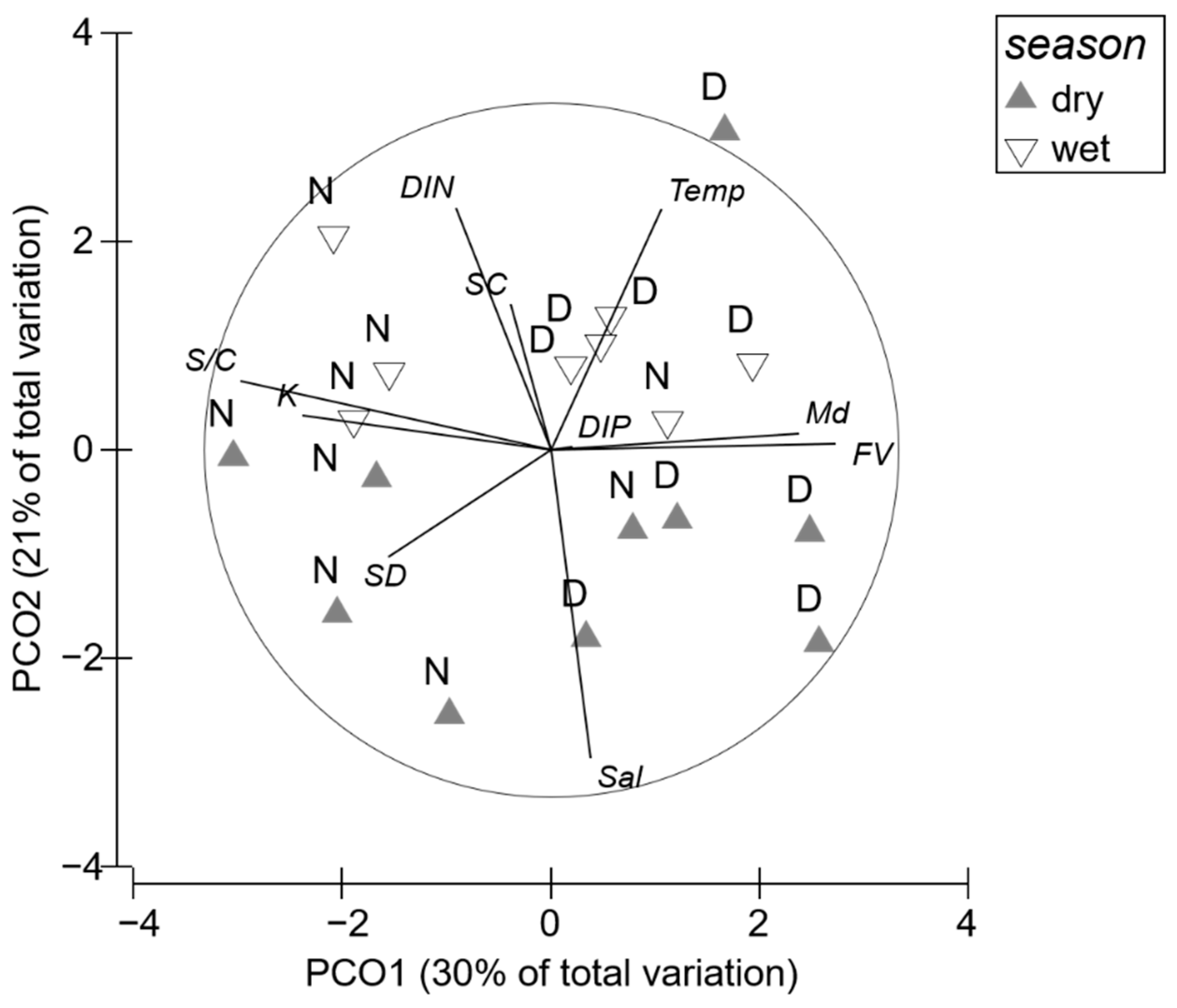
3.1. Environmental Factors

During low tide, seawater temperature and salinity averaged 31.9 °C and 33.1, respectively, in the wet season (summer and autumn) and 28.1 °C and 34.7, respectively, in the dry season (winter and spring) (Table 1). There was no significant difference in the light extinction coefficient between sites and seasons (Table S1). The seawater DIN concentration was 2–3 times higher in the wet season than in the dry season. However, the seawater DIP concentration did not differ between sites or seasons.
The relative flow velocity was faster in Dakwan than in Nanwan, particularly in the dry season (Table S2), suggesting that the seawater was more disturbed by waves and tidal currents during the northeast monsoon. Consequently, sediment grain size was larger in Dakwan than in Nanwan. Conversely, the silt/clay content was higher in Nanwan (4.9%) than in Dakwan (1.9%). The sediments at both sites were poorly sorted.
At a low tide in the high-elevation site Dakwan, the water level of the seagrass bed increased with the distance from the coast and to the right of the fixed transect until the water level was >36 cm (Figure 2a). Most of the water level of the seagrass bed was <9 cm. The seawater became deeper at a distance of 30 m to the right from the fixed transect. The water level of the seagrass bed in the low-elevation site Nanwan was deeper than that in Dakwan, as almost all the water levels were >9 cm (Figure 2c). The deepest water level of the seagrass bed in Nanwan reached 58 cm at a distance of 18 m from the coast.
Sediment depth also varied across the seagrass bed in Dakwan (Figure 2b). In general, the sediments were deeper within 6 m from the coast. The sediments were 50% deeper in Nanwan than in Dakwan. One-third of the sediments in Nanwan were >5 cm deep (Figure 2d). The greatest sediment depth of the seagrass bed in Nanwan reached 17 cm.

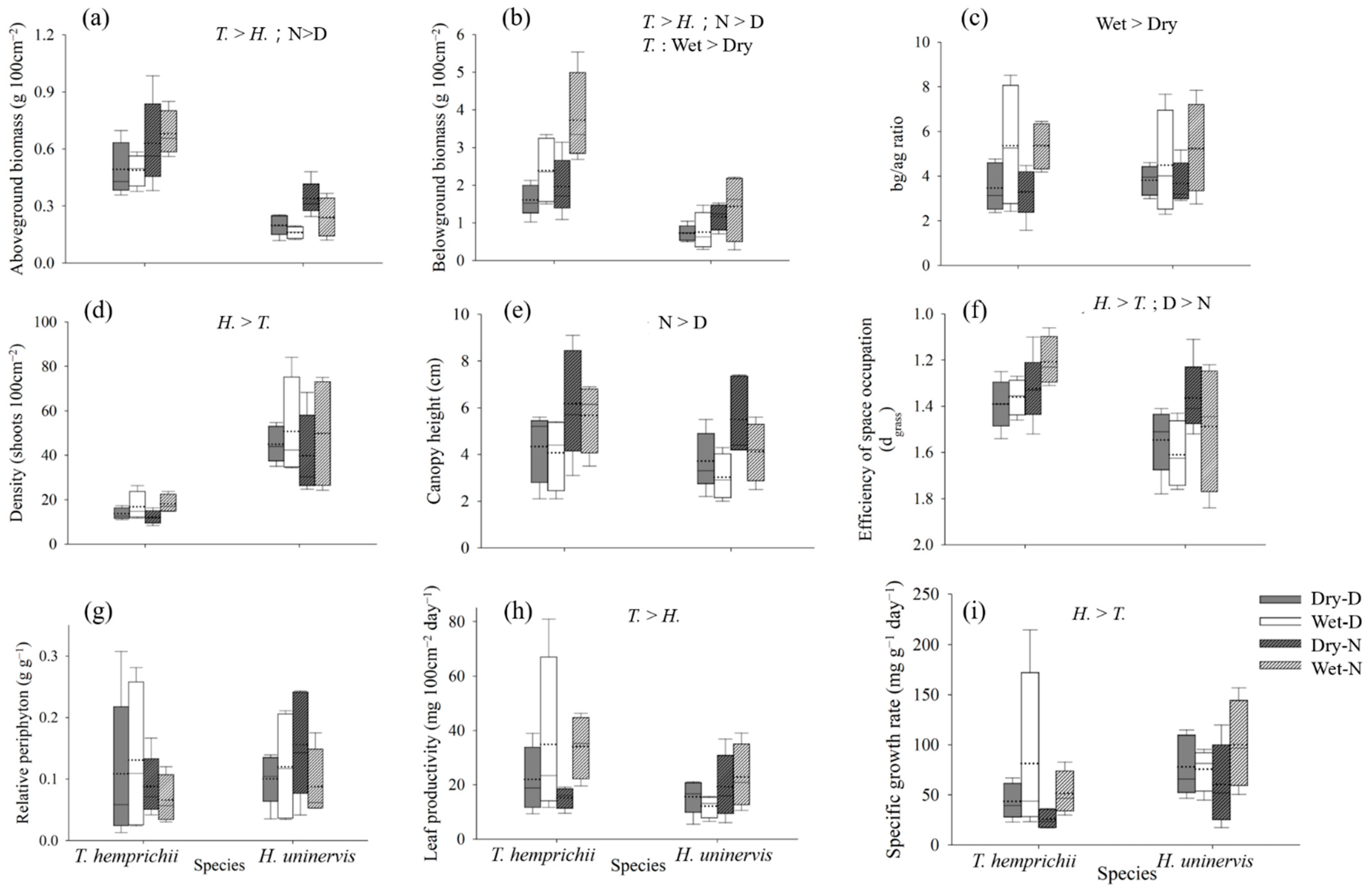
3.2. Seagrass Variables

The aboveground biomass of T. hemprichii averaged approximately 3 times that of H. uninervis (Figure 3a). Similarly, the belowground biomass of T. hemprichii averaged approximately 2.7 times that of H. uninervis (Figure 3b). There was seasonal variation in the belowground biomass of T. hemprichii, in which the belowground biomass was higher in the wet season than in the dry season. The bg/ag ratios of both seagrass species were significantly higher in the wet season than in the dry season (Figure 3c).
The shoot density of H. uninervis averaged approximately 3 times that of T. hemprichii (Figure 3d). However, the canopy height of T. hemprichii averaged 1 cm higher than that of H. uninervis (Figure 3e). The space occupation by T. hemprichii was more efficient than that by H. uninervis (Figure 3f). In addition, the space occupation by both seagrass species in Nanwan was more efficient than in Dakwan.
There were no significant differences in periphyton biomass (not shown) or relative periphyton biomass between sites, seasons and seagrass species (Figure 3g). It was noted that the pattern of seasonal variation in relative periphyton biomass differed at the two sites. In Dakwan, the relative periphyton biomass was lower in the dry season than in the wet season, whereas the relative periphyton biomass in Nanwan was lower in the wet season.
The leaf productivity of T. hemprichii was significantly higher than that of H. uninervis (Figure 3h). However, the specific growth rate of H. uninervis averaged approximately 2 times faster than that of T. hemprichii (Figure 3i). The specific growth rate of both seagrass leaves was faster in the wet season than in the dry season.

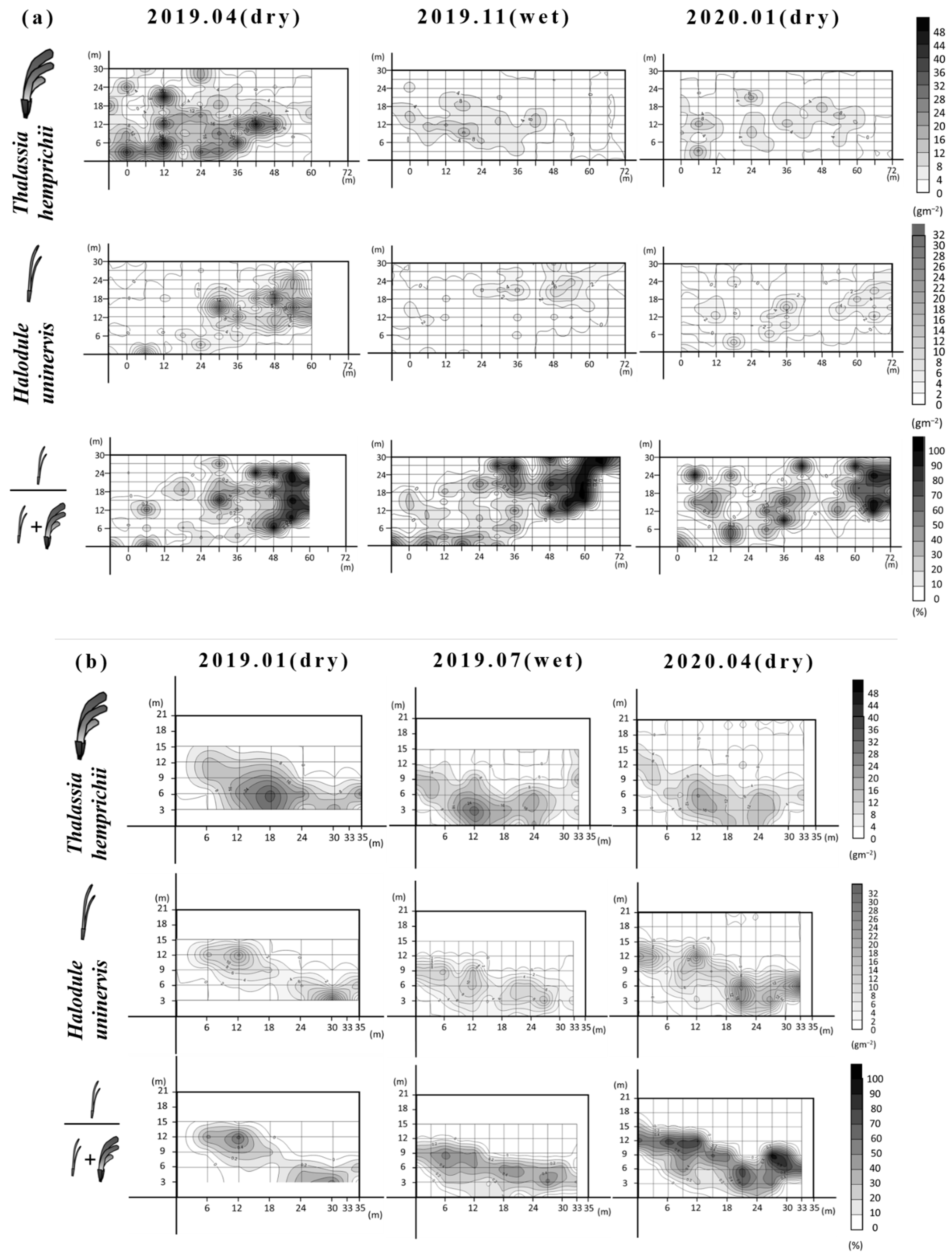
3.3. High-Resolution Mapping of Seagrass Biomass Dynamics

In Dakwan, the cover area of seagrass beds increased from April (the end of the dry season) to November (the end of the wet season) in 2019 (Table 2). However, the mean biomass density of T. hemprichii and H. uninervis decreased remarkably. In January (the dry season) in 2020, the cover area of seagrass beds decreased again. However, the mean biomass density of T. hemprichii and H. uninervis increased slightly. Briefly, the biomass density of both seagrass species in Dakwan was higher in the dry season. However, the cover area of seagrass beds was larger in the wet season.
The dominant area of seagrass species indicated the area where the seagrass species contributed > 50% of the total biomass in the seagrass beds. T. hemprichii was the dominant species at both sites year-round as the percentage of the dominant area was >72% (Table 2). However, the distribution of both species in the seagrass bed of Dakwan was distinct (Figure 4a). The distribution of H. uninervis was dominant in the water > 18 cm deep, whereas the distribution of T. hemprichii was dominant in the water < 12 cm deep. There was a clear seasonal succession in the community structure of seagrass beds. The dominance of H. uninervis moved to shallower water in the wet season and then moved back to deeper water in the dry season.
In Nanwan, the cover area of seagrass beds increased slightly from January (the dry season) to July (the wet season) in 2019 (Table 2). However, the mean biomass density of T. hemprichii decreased, but the biomass density of H. uninervis increased slightly. In April (the end of the dry season) in 2020, the cover area of seagrass beds increased further. The mean biomass density of T. hemprichii decreased, but the biomass density of H. uninervis increased further. Briefly, the cover area of seagrass beds in Nanwan was increasing during the study period. While the dominance of H. uninervis was increasing, the dominance of T. hemprichii was decreasing.
Inconsistent with the distinct distribution pattern of seagrass species in Dakwan, both species were well-mixed in Nanwan. Although H. uninervis was dominant in the water > 18 cm deep and T. hemprichii was dominant in the water < 12 cm deep, the dominance of H. uninervis increased from the first dry season to the second dry season, as most of the seagrass beds in Nanwan were in the water > 18 cm deep (Table 2). Compared to the seasonal succession pattern in Dakwan, the seasonal pattern in the community structure of the seagrass bed was not clear in Nanwan.

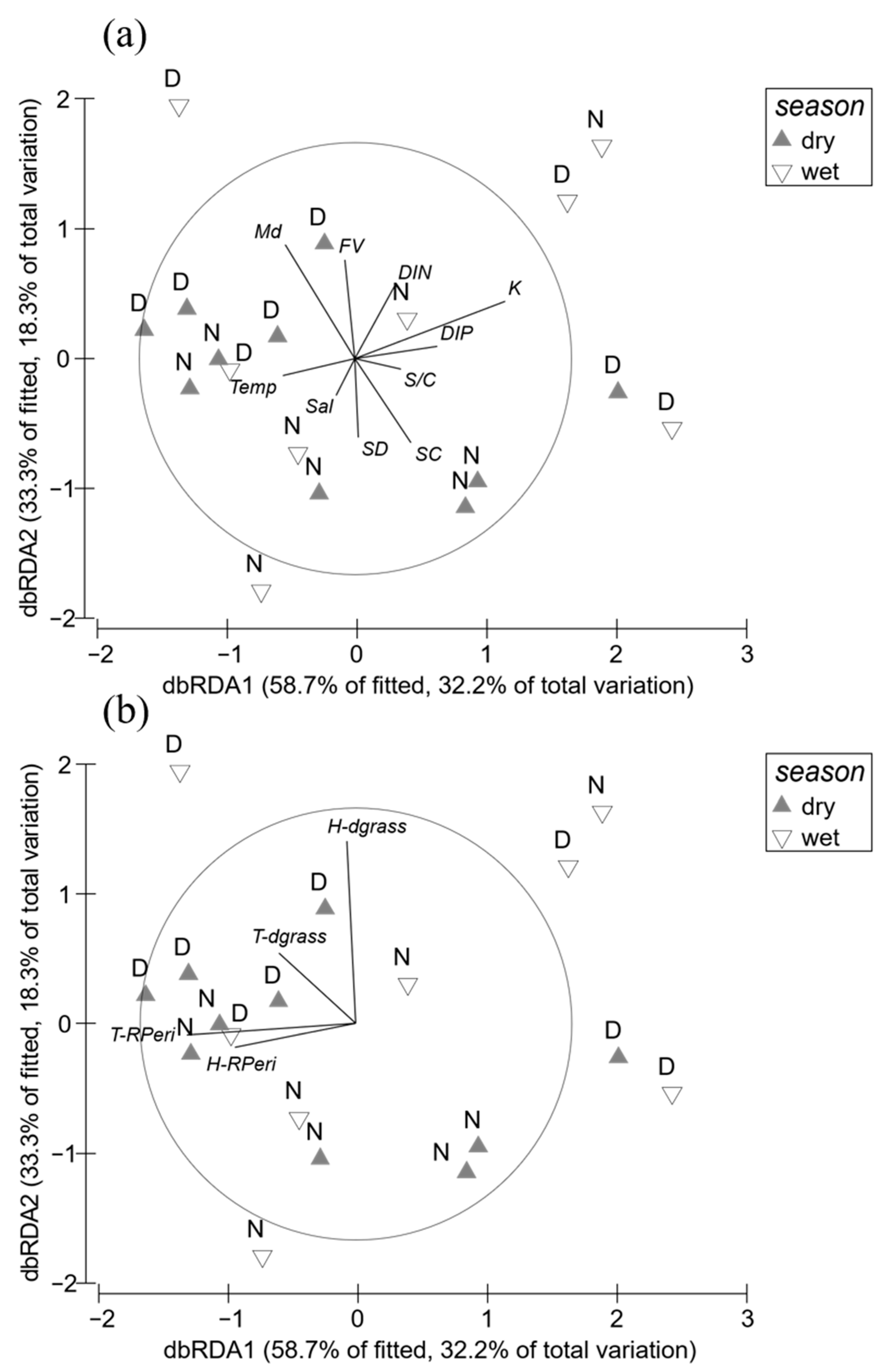
3.4. Relationship between Seagrass Variables and Environmental Factors

A PCoA was used to assess the most influential environmental factors for the seasonal and spatial patterns of seagrass variables at the two sites. The first (PCO1) and second (PCO2) axes of the PCoA explained a total of 51% of the variation in the environmental factors (Figure 5). The axis of PCO1 explaining 30% of the total variation separated the samples into the right side collected from Dakwan, and the left side from Nanwan. The axis of PCO2 explaining 22% of the total variation separated the samples into the upper part collected from the wet season and the lower part from the dry season. The samples collected from the wet season were characterized by higher temperatures, DIN concentrations and sorting coefficients, whereas the dry season samples were characterized by higher salinity values. While the samples collected in Dakwan featured faster flow velocity and larger grain size, the samples collected in Nanwan featured a higher silt/clay content in the sediment, light extinction coefficient and sediment depth.
The dbRDA results showed that there was a positive correlation between the dgrass of T. hemprichii and the periphyton biomass, whereas there was no correlation between the dgrass of H. uninervis and the periphyton biomass (Figure 6). This result suggested that periphyton imposed a negative effect on T. hemprichii but little effect on H. uninervis. There was a positive correlation between the relative flow velocity and the dgrass of H. uninervis, and negative correlations between sediment depth and the sorting coefficient and the dgrass of H. uninervis. This suggested that the conditions of faster flow velocity, shallower sediment depth and smaller sorting coefficient constrained the growth of H. uninervis. Although similar correlations also occurred in the dgrass of T. hemprichii, the results of dbRDA suggested that the negative effects of sediment depth and sorting coefficient on H. uninervis were more serious than those on T. hemprichii.

4. Discussion

4.1. Competition in Seagrass Community

Interspecific competition and resource availability are often the main factors structuring seagrass communities [34]. The possible mechanism for the shift of the dominance of T. hemprichii in the seagrass beds can be partly referred from the competition between In the Caribbean, Thalassia testudinum and Halodule wrightii, which are the sister species of T. hemprichii and H. uninervis in the Caribbean. The leaf growth of T. testudinum and H. wrightii is affected mainly by their competition when nutrients are not limited in the environment [35]. The turnover rate of the belowground part is faster for the early-successional seagrass.
H. wrightii so that it is capable of expanding to new space. However, the lifespan of the late-successional seagrass T. testudinum is longer, which can avoid the expansion of H. wrightii to the space of T. testudinum [36]. The dominance of the larger seagrass T. testudinum is possibly due to the shading of the light reaching the smaller seagrass H. wrightii [37]. H. wrightii is capable of adapting to low irradiance [38], so H. wrightii is often observed growing in mixed seagrass beds, as in our case of H. uninervis in southern Taiwan [39]. The decline in T. testudinum at fertilized sites is outcompeted by H. wrightii in response to nutrient enrichment [40]. The faster growing seagrass H. wrightii may even inhibit the restoration of T. testudinum [41]. Gaubert-Boussarie et al. [42] indicated that the feasibility of irradiance and nutrients may coregulate the coverage and biomass of T. testudinum and H. wrightii in the community. Robbins et al. [43] further indicated that the shift of T. testudinum and H. wrightii in the community of mixed seagrass beds is not simply driven by water depth but also involves flow velocity. These results suggested that the availability of irradiance and nutrients and hydrodynamic movement might affect the competition of T. hemprichii and H. uninervis in the community.

4.2. Differential Response of Seagrasses to Environments

Seagrasses in shallow water have to cope with drought, high irradiances and temperatures [44]. In this study, T. hemprichii was more dominant in the seagrass beds because it is more resistant to drought than H. uninervis [39]. The dominance of H. uninervis in the water >18 cm deep likely stems from its faster growth rates and its ability to effectively compete for space [39]. The wet season is characterized by higher temperatures, precipitation levels and seawater DIN concentrations, which can increase the leaf and belowground production of both seagrass species [6,8,20]. Consequently, the cover area of both seagrass species increased in the wet season, which supports our hypothesis that both seagrass species will respond positively to warming and increased precipitation. However, the specific growth rate of H. uninervis is faster than that of T. hemprichii. The rhizome productivity of H. uninervis is even 5 times higher than that of T. hemprichii [8]. The turnover rates of both aboveground and belowground parts of H. uninervis are higher than those of T. hemprichii [8], so that H. uninervis is capable of expanding more space than T. hemprichii.
In the dry season, the northeast monsoon prevailed, which imposed drought stress on seagrasses, particularly H. uninervis [39]. This might reduce the aboveground biomass when exposed to air at low tide [45]. Additionally, the larger seagrass T. hemprichii was more dominant in the water with faster flow velocity than the smaller seagrass H. uninervis. This was evident by the dbRDA results that the dgrass of H. uninervis correlated positively with flow velocity and negatively with sediment depth and sorting coefficient. The faster flow velocity in the high-elevation site (Dakwan) might disturb the sediment frequently, as observed by Congdon et al. [18], and constrain the further expansion of H. uninervis to shallow water in the wet season when the northeast monsoon ceased. Chiu et al. [46] quantified the carbon budget of T. hemprichii leaves in Dakwan and concluded that 32% of leaf production was exported to neighboring coral reefs. The faster flow velocity in Dakwan has thus resulted in lower sedimentation rates than in Nanwan over the past 20 years [8]. This may be the reason why the dominance of H. uninervis was lower (15–22%) in Dakwan than in the relatively sheltered Nanwan (up to 28%).
The high-resolution mapping on the seagrass bed of Dakwan further showed a clear seasonal succession in dominant species (Table 2). The dominance area of H. uninervis shifted from 16.9% in the dry season to 22.0% in the wet season (23% increase), and then back to 15.2% in the dry season. Simultaneously, the dominance of T. hemprichii shifted correspondingly in the dry and wet seasons. The wet season in southern Taiwan is characterized by higher temperature, precipitation levels and seawater DIN concentrations. The observed seasonal succession pattern supports the hypothesis [6] that T. hemprichii shoots are more vulnerable to higher precipitation levels and DIN concentrations in the wet season, and particularly heavy precipitation during La Niña years. This may have been due to competition for space with H. uninervis, as the more intense precipitation may reduce drought stress at low tide, and the high DIN concentration may stimulate the growth of H. uninervis; both can increase its competition over T. hemprichii within the community [6].
Deeper water may also reduce the drought stress of H. uninervis at low tide and increase its competition over T. hemprichii within the community. In the low-elevation site (Nanwan), the dominance of T. hemprichii decreased remarkably from 98.3% in 2019 to 72.1% in early 2020 (Table 2). Conversely, the dominance of H. uninervis increased from 1.7% in 2019 to 27.9% in 2020. This suggested that the carbon sequestration capacity of the seagrass beds will decrease, as T. hemprichii is capable of storing more carbon in the sediments. The results also suggested that the effects of deeper water were more remarkable than the effects of warming and higher precipitation, as the seasonal succession pattern in the wet season was masked by the effects of deeper water (>9 cm at low tide) in Nanwan; therefore, the seasonal succession pattern was not clear.
The flushing of land-based nutrients into the sea by heavy rainfall in the wet season may impose stress on seagrasses [6]. The overgrowth of periphyton has long been reported to pose negative impacts on seagrasses [47,48]. La Nafie et al. [45] indicated that the seagrass beds of Zostera noltii would decline in response to the joint effects of waves and high nutrient loads, which may decrease the mechanical properties and survival. Periphyton biomass was observed to grow on both seagrass species at both sites. The increase in periphyton biomass on the seagrasses at the two sites can be attributed to the loading of anthropogenic wastewater [49]. Periphyton biomass on seagrasses is often reduced by water flow velocity [50] and herbivory [51,52]. In this study, the periphyton biomass on seagrasses showed inconsistent seasonal patterns at the two sites, which appeared to be affected by the monsoon. Dakwan is located on the windward side of the northeast monsoon, whereas Nanwan is located on the windward side of the southwest monsoon. The periphyton biomass on the seagrasses at both sites was lower during the period when the windward monsoon prevailed. The periphyton biomass was lower in Dakwan in the dry season, but it was lower in Nanwan in the wet season. This suggested that flow velocity caused by monsoons, particularly the northeast monsoon, was a main factor removing periphyton on the seagrasses in the high-elevation site.
However, according to the dbRDA results of the efficiency of space occupation analysis, the periphyton biomass had a negative impact on T. hemprichii but little negative effect on H. uninervis. This differential effect of periphyton biomass can be attributed to the distinct turnover rates of the two seagrass species. In addition to grazing and waves, seagrass leaf turnover is also a main mechanism to reduce periphyton growing on the leaves [53]. The lower growth and slower turnover rates of the leaves of the late-successional seagrass T. hemprichii would be more difficult to reduce periphyton in Nanwan, where flow velocity was slower and nutrient loads were higher in the wet season. Conversely, the competitive capability of the early-successional seagrass H. uninervis with higher growth and faster turnover rates of leaves and belowground parts [8] would increase, especially in Nanwan, where the seawater was deeper and drought stress was much lower. While the shedding of old leaves may also be a primary means of reducing the impacts of periphyton overgrowth on seagrasses, H. uninervis would be less detrimental than T. hemprichii due to the former’s faster leaf growth and shorter turnover time.

5. Conclusions

The high-resolution mapping of seagrass biomass dynamics showed that T. hemprichii was the dominant species in the study sites year round. In the high-elevation site, the distribution of both species was distinct and showed a clear seasonal succession. The dominance of H. uninervis moved to shallower water in the wet season and then moved back to deeper water in the dry season. However, the seasonal pattern was not clear in the low-elevation site. Our observations suggested that four possible mechanisms might be involved in the dominance shift in the shallow seagrass beds: (1) deeper water or more intense precipitation might reduce the drought stress of H. uninervis at low tide and enhance its competition; (2) the growth of H. uninervis might be stimulated more by the flushing of land-based nutrients in the wet season; (3) faster flow velocity might constrain the expansion of H. uninervis to shallower water; (4) faster flow velocity might reduce the impacts of periphyton overgrowth on T. hemprichii and maintain the dominance of T. hemprichii in the community. This study demonstrated that seagrass species responded differently to environmental drivers, showing the importance of considering species-specific responses when predicting the effects of climate change-associated factors on seagrasses.

Supplementary Materials

Supplementary data associated with this article can be found online at https://www.mdpi.com/article/10.3390/d14110999/s1. Table S1: Two-way ANOVA results of season (wet vs. dry) and site (Dakwan vs. Nanwan) on environmental parameters collected in southern Taiwan. Table S2: The results of Student’s t test, Welch’s t test and Mann-Whitney U test of the effects of season (wet vs. dry) and site (Dakwan vs. Nanwan) on flow velocity and salinity measured in southern Taiwan. Table S3: Three-way ANOVA results of season (dry vs. wet), site (Dakwan vs. Nanwan) and species (Thalassia hemprichii vs. Halodule uninervis) on seagrass variables measured in southern Taiwan.

Author Contributions

K.-Y.C. and H.-J.L. conceived and designed the study, carried out the field work and contributed to the data analysis, interpretation and manuscript writing. All authors have read and agreed to the published version of the manuscript.

Funding

This study was financially supported by the “Innovation and Development Center of Sustainable Agriculture” from The Featured Areas Research Center Program within the Higher Education Sprout Project by the Ministry of Education (MOE) of Taiwan.

Institutional Review Board Statement

Not applicable.

Data Availability Statement

The data presented in this study are available on request from the corresponding author.

Acknowledgments

We thank Yi-Fang Zou, Yu-Chen Kao, Meng-Quen Chou, Ming-Ru Song and Yu-Hung Zhou for field assistance.

Conflicts of Interest

The authors declare no competing interest.

References

  1. Nelleman, C.; Corcoran, E.; Duarte, C.M.; Valdes, L.; DeYoung, C.; Fonseca, L.; Grimsditch, G. Blue Carbon: The Role of Healthy Oceans in Binding Carbon; UNEP/FAO/UNESCO/IUCN/CSIC: Madrid, Spain, 2008. [Google Scholar]
  2. Laffoley, D.; Grimsditch, G.D. The Management of Natural Coastal Carbon Sinks; IUCN: Gland, Vaud, Switzerland, 2009. [Google Scholar]
  3. Davidson, N.C.; Finlayson, C.M. Updating global coastal wetland areas presented in Davidson and Finlayson (2018). Mar. Freshw. Res. 2019, 70, 1195–1200. [Google Scholar] [CrossRef]
  4. Lin, W.-J.; Wu, J.; Lin, H.-J. Contribution of unvegetated tidal flats to coastal carbon flux. Glob. Chang. Biol. 2020, 26, 3443–3454. [Google Scholar] [CrossRef]
  5. Mukai, H. Biogeography of the tropical seagrasses in the western Pacific. Mar. Freshw. Res. 1993, 44, 1–17. [Google Scholar] [CrossRef]
  6. Lin, H.-J.; Lee, C.-L.; Peng, S.-E.; Hung, M.-C.; Liu, P.-J.; Mayfield, A.B. The effects of El Niño-Southern Oscillation events on intertidal seagrass beds over a long-term timescale. Glob. Chang. Biol. 2018, 24, 4566–4580. [Google Scholar] [CrossRef] [PubMed]
  7. Huang, Y.-H.; Lee, C.-L.; Chung, C.-Y.; Hsiao, S.-C.; Lin, H.-J. Carbon budgets of multispecies seagrass beds at Dongsha Island in the South China Sea. Mar. Environ. Res. 2015, 106, 92–102. [Google Scholar] [CrossRef] [PubMed]
  8. Zou, Y.-F.; Chen, K.-Y.; Lin, H.-J. Significance of belowground production to the long-term carbon sequestration of intertidal seagrass beds. Sci. Total Environ. 2021, 800, 149579. [Google Scholar] [CrossRef] [PubMed]
  9. Friedlingstein, P.; Jones, M.W.; O’Sullivan, M.; Andrew, R.M.; Bakker, D.C.; Hauck, J.; Le Quéré, C.; Peters, G.P.; Peters, W.; Pongratz, J. Global carbon budget 2021. Earth Syst. Sci. Data 2022, 14, 1917–2005. [Google Scholar] [CrossRef]
  10. Arias, P.; Bellouin, N.; Coppola, E.; Jones, R.; Krinner, G.; Marotzke, J.; Naik, V.; Palmer, M.; Plattner, G.-K.; Rogelj, J.; et al. Climate Change 2021: The Physical Science Basis. Contribution of Working Group I to the Sixth Assessment Report of the Intergovernmental Panel on Climate Change; Technical Summary. In Proceedings of the Intergovernmental Panel on Climate Change AR6; Cambridge University Press: Cambridge, UK; New York, NY, USA, 2021. [Google Scholar]
  11. Mazarrasa, I.; Samper-Villarreal, J.; Serrano, O.; Lavery, P.S.; Lovelock, C.E.; Marbà, N.; Duarte, C.M.; Cortés, J. Habitat characteristics provide insights of carbon storage in seagrass meadows. Mar. Pollut. Bull. 2018, 134, 106–117. [Google Scholar] [CrossRef] [PubMed]
  12. Krause-Jensen, D.; Duarte, C.M. Expansion of vegetated coastal ecosystems in the future Arctic. Front. Mar. Sci. 2014, 1, 77. [Google Scholar] [CrossRef] [Green Version]
  13. Clausen, K.K.; Krause-Jensen, D.; Olesen, B.; Marbà, N. Seasonality of eelgrass biomass across gradients in temperature and latitude. Mar. Ecol. Prog. Ser. 2014, 506, 71–85. [Google Scholar] [CrossRef]
  14. Collier, C.J.; Langlois, L.; Ow, Y.; Johansson, C.; Giammusso, M.; Adams, M.P.; O’Brien, K.R.; Uthicke, S. Losing a winner: Thermal stress and local pressures outweigh the positive effects of ocean acidification for tropical seagrasses. New Phytol. 2018, 219, 1005–1017. [Google Scholar] [CrossRef] [PubMed] [Green Version]
  15. George, R.; Gullström, M.; Mangora, M.M.; Mtolera, M.S.; Björk, M. High midday temperature stress has stronger effects on biomass than on photosynthesis: A mesocosm experiment on four tropical seagrass species. Ecol. Evol. 2018, 8, 4508–4517. [Google Scholar] [CrossRef] [PubMed]
  16. Saunders, M.I.; Leon, J.; Phinn, S.R.; Callaghan, D.P.; O’Brien, K.R.; Roelfsema, C.M.; Lovelock, C.E.; Lyons, M.B.; Mumby, P.J. Coastal retreat and improved water quality mitigate losses of seagrass from sea level rise. Glob. Chang. Biol. 2013, 19, 2569–2583. [Google Scholar] [CrossRef]
  17. Short, F.T.; Neckles, H.A. The effects of global climate change on seagrasses. Aquat. Bot. 1999, 63, 169–196. [Google Scholar] [CrossRef]
  18. Congdon, V.M.; Bonsell, C.; Cuddy, M.R.; Dunton, K.H. In the wake of a major hurricane: Differential effects on early vs. late successional seagrass species. Limnol. Oceanogr. Lett. 2019, 4, 155–163. [Google Scholar] [CrossRef] [Green Version]
  19. Liu, P.-J.; Chang, H.-F.; Mayfield, A.B.; Lin, H.-J. Assessing the Effects of Ocean Warming and Acidification on the Seagrass Thalassia hemprichii. J. Mar. Sci. Eng. 2022, 10, 714. [Google Scholar] [CrossRef]
  20. Lin, H.-J.; Shao, K.-T. Temporal changes in the abundance and growth of intertidal Thalassia hemprichii seagrass beds in southern Taiwan. Bot. Bull. Acad. Sin. 1998, 39, 191–198. [Google Scholar]
  21. Lee, C.-L.; Lin, W.-J.; Liu, P.-J.; Shao, K.-T.; Lin, H.-J. Highly productive tropical seagrass beds support diverse consumers and a large organic carbon pool in the sediments. Diversity 2021, 13, 544. [Google Scholar] [CrossRef]
  22. Hsieh, H.-L. Spatial and temporal patterns of polychaete communities in a subtropical mangrove swamp: Influences of sediment and microhabitat. Mar. Ecol. Prog. Ser. 1995, 127, 157–167. [Google Scholar] [CrossRef]
  23. Murphy, J.; Riley, J.P. A modified single solution method for the determination of phosphate in natural waters. Anal. Chim. Acta 1962, 27, 31–36. [Google Scholar] [CrossRef]
  24. Pai, S.-C.; Tsau, Y.-J.; Yang, T.-I. pH and buffering capacity problems involved in the determination of ammonia in saline water using the indophenol blue spectrophotometric method. Anal. Chim. Acta 2001, 434, 209–216. [Google Scholar] [CrossRef]
  25. Jenkins, D.; Medsker, L.L. Brucine Method for the Determination of Nitrate in Ocean, Estuarine, and Fresh Waters. Anal. Chem. 1964, 36, 610–612. [Google Scholar] [CrossRef]
  26. Pai, S.-C.; Yang, C.-C.; Riley, J.P. Formation kinetics of the pink azo dye in the determination of nitrite in natural waters. Anal. Chim. Acta 1990, 232, 345–349. [Google Scholar] [CrossRef]
  27. Doty, M.S. Measurement of water movement in reference to benthic algal growth. Bot. Mar. 1971, 14, 32–35. [Google Scholar] [CrossRef]
  28. Lin, H.-J.; Wang, T.-C.; Su, H.-M.; Hung, J.-J. Relative importance of phytoplankton and periphyton on oyster-culture pens in a eutrophic tropical lagoon. Aquaculture 2005, 243, 279–290. [Google Scholar] [CrossRef]
  29. Short, F.T.; Coles, R.G. Global Seagrass Research Methods; Elsevier: Amsterdam, The Netherlands, 2003. [Google Scholar]
  30. Vieira, V.M.; Lopes, I.E.; Creed, J.C. The biomass–density relationship in seagrasses and its use as an ecological indicator. BMC Ecol. 2018, 18, 44. [Google Scholar] [CrossRef] [PubMed] [Green Version]
  31. Clarke, K.R.; Warwick, R. Change in Marine Communities: An Approach to Statistical Analysis and Interpretation; PRIMER-E: Plymouth, UK, 2001. [Google Scholar]
  32. Clarke, K.R.; Gorley, R.N. PRIMER v6: User Manual/Tutorial; PRIMER-E: Plymouth, UK, 2006. [Google Scholar]
  33. Anderson, M.J.; Gorley, R.N.; Clarke, K.R. PERMANOVA+ for PRIMER: Guide to Software and Statistical Methods; PRIMER-E: Plymouth, UK, 2008. [Google Scholar]
  34. Tilman, D. The resource-ratio hypothesis of plant succession. Am. Nat. 1985, 125, 827–852. [Google Scholar] [CrossRef]
  35. Rose, C.D.; Dawes, C.J. Effects of community structure on the seagrass Thalassia testudinum. Mar. Ecol. Prog. Ser. 1999, 184, 83–95. [Google Scholar] [CrossRef] [Green Version]
  36. Gallegos, M.E.; Merino, M.; Rodriguez, A.; Marbà, N.; Duarte, C.M. Growth patterns and demography of pioneer Caribbean seagrasses Halodule wrightii and Syringodium filiforme. Mar. Ecol. Prog. Ser. 1994, 109, 99–104. [Google Scholar] [CrossRef]
  37. Zieman, J.C. The Ecology of the Seagrasses of South Florida: A Community Profile; Department of the Interior, US Fish and Wildlife Service: Washington, DC, USA, 1982.
  38. Iverson, R.L.; Bittaker, H.F. Seagrass distribution and abundance in Eastern Gulf of Mexico coastal waters. Estuar. Coast. Shelf Sci. 1986, 22, 577–602. [Google Scholar] [CrossRef]
  39. Lan, C.-Y.; Kao, W.-Y.; Lin, H.-J.; Shao, K.-T. Measurement of chlorophyll fluorescence reveals mechanisms for habitat niche separation of the intertidal seagrasses Thalassia hemprichii and Halodule uninervis. Mar. Biol. 2005, 148, 25–34. [Google Scholar] [CrossRef]
  40. Fourqurean, J.W.; Powell, G.V.; Kenworthy, W.J.; Zieman, J.C. The effects of long-term manipulation of nutrient supply on competition between the seagrasses Thalassia testudinum and Halodule wrightii in Florida Bay. Oikos 1995, 72, 349–358. [Google Scholar] [CrossRef] [Green Version]
  41. Furman, B.T.; Merello, M.; Shea, C.P.; Kenworthy, W.J.; Hall, M.O. Monitoring of physically restored seagrass meadows reveals a slow rate of recovery for Thalassia testudinum. Restor. Ecol. 2019, 27, 421–430. [Google Scholar] [CrossRef]
  42. Gaubert-Boussarie, J.; Altieri, A.H.; Duffy, J.E.; Campbell, J.E. Seagrass structural and elemental indicators reveal high nutrient availability within a tropical lagoon in Panama. PeerJ 2021, 9, e11308. [Google Scholar] [CrossRef]
  43. Robbins, B.D.; Bell, S.S. Dynamics of a subtidal seagrass landscape: Seasonal and annual change in relation to water depth. Ecology 2000, 81, 1193–1205. [Google Scholar] [CrossRef]
  44. Jupp, B.; Durako, M.J.; Kenworthy, W.; Thayer, G.; Schillak, L. Distribution, abundance, and species composition of seagrasses at several sites in Oman. Aquat. Bot. 1996, 53, 199–213. [Google Scholar] [CrossRef]
  45. La Nafie, Y.A.; De Los Santos, C.B.; Brun, F.G.; Van Katwijk, M.M.; Bouma, T.J. Waves and high nutrient loads jointly decrease survival and separately affect morphological and biomechanical properties in the seagrass Zostera noltii. Limnol. Oceanogr. 2012, 57, 1664–1672. [Google Scholar] [CrossRef] [Green Version]
  46. Chiu, S.-H.; Huang, Y.-H.; Lin, H.-J. Carbon budget of leaves of the tropical intertidal seagrass Thalassia hemprichii. Estuar. Coast. Shelf Sci. 2013, 125, 27–35. [Google Scholar] [CrossRef]
  47. Burkholder, J.M.; Tomasko, D.A.; Touchette, B.W. Seagrasses and eutrophication. J. Exp. Mar. Biol. Ecol. 2007, 350, 46–72. [Google Scholar] [CrossRef]
  48. Camacho, R.; Houk, P. Decoupling seasonal and temporal dynamics of macroalgal canopy cover in seagrass beds. J. Exp. Mar. Biol. Ecol. 2020, 525, 151310. [Google Scholar] [CrossRef]
  49. Lin, H.-J.; Wu, C.-Y.; Kao, S.-J.; Kao, W.-Y.; Meng, P.-J. Mapping anthropogenic nitrogen through point sources in coral reefs using δ15N in macroalgae. Mar. Ecol. Prog. Ser. 2007, 335, 95–109. [Google Scholar] [CrossRef]
  50. Strand, J.A.; Weisner, S.E. Wave exposure related growth of epiphyton: Implications for the distribution of submerged macrophytes in eutrophic lakes. Hydrobiologia 1996, 325, 113–119. [Google Scholar] [CrossRef]
  51. Christianen, M.J.; Govers, L.L.; Bouma, T.J.; Kiswara, W.; Roelofs, J.G.; Lamers, L.P.; van Katwijk, M.M. Marine megaherbivore grazing may increase seagrass tolerance to high nutrient loads. J. Ecol. 2012, 100, 546–560. [Google Scholar] [CrossRef]
  52. Lee, C.-L.; Huang, Y.-H.; Chung, C.-Y.; Lin, H.-J. Tidal variation in fish assemblages and trophic structures in tropical Indo-Pacific seagrass beds. Zool. Stud. 2014, 53, 56. [Google Scholar] [CrossRef] [Green Version]
  53. Nelson, W.G. Development of an epiphyte indicator of nutrient enrichment: Threshold values for seagrass epiphyte load. Ecol. Indic. 2017, 74, 343–356. [Google Scholar] [CrossRef] [PubMed]
Figure 1. The seagrass beds at low tide in (a) Dakwan, which is the windward side of the northeast monsoon in winter; and (b) Nanwan, which is the windward side of the southwest monsoon in summer.
Diversity 14 00999 g001
Figure 2. (a) Water depth (cm) and (b) sediment depth (cm) in the seagrass bed of Dakwan during a low tide. (c) Water depth (cm) and (d) sediment depth (cm) in the seagrass bed of Nanwan during a low tide. The x-axis was the distance (m) from the fixed transect (#0), and the y-axis was the distance from the coast.
Diversity 14 00999 g002
Figure 3. Normal quantile plots of (a) aboveground biomass, (b) belowground biomass, (c) bg/ag ratio, (d) density, (e) canopy height, (f) efficiency of space occupation, (g) relative periphyton biomass, (h) leaf productivity, and (i) specific growth rate of Thalassia hemprichii and Halodule uninervis measured in the dry and wet seasons in Dakwan (D) and Nanwan (N) from 2018 to 2020. Post-hoc differences (see Table S3) have been mentioned at the top of each panel when species-, site- and/or season-related differences were detected in the three-way ANOVA.
Diversity 14 00999 g003
Figure 4. High-resolution mapping of the biomass density of Thalassia hemprichii and Halodule uninervis and the proportion of H. uninervis compared to the total biomass density of T. hemprichii and H. uninervis in the seagrass beds of (a) Dakwan and (b) Nanwan. The x-axis was the distance (m) from the fixed transect (#0), and the y-axis was the distance from the coast.
Diversity 14 00999 g004
Figure 5. PCoA of the environmental factors measured in Dakwan (D) and Nanwan (N) in the dry and wet seasons. Temp: seawater temperature; Sal: seawater salinity; DIN: dissolved inorganic nitrogen concentration; DIP: dissolved inorganic phosphorus; K: light extinction coefficient; FV: seawater flow velocity; SD: sediment depth; Md: sediment grain size; S/C: sediment silt/clay content (%); SC: sorting coefficient.
Diversity 14 00999 g005
Figure 6. dbRDA plots showing the relationships between (a) environmental factors, (b) efficiency of space occupation (dgrass) and relative periphyton biomass (RPeri) and seagrass variables (Thalassia hemprichii and Halodule uninervis) measured in Dakwan (D) and Nanwan (N) in the dry and wet seasons. Temp: seawater temperature; Sal: seawater salinity; DIN: dissolved inorganic nitrogen concentration; DIP: dissolved inorganic phosphorus concentration; K: light extinction coefficient; FV: seawater flow velocity; SD: sediment depth; Md: sediment grain size; S/C: silt/clay content (%); and SC: sorting coefficient.
Diversity 14 00999 g006
Table 1. Water, sediment and seagrass variables determined in the seagrass beds of Dakwan and Nanwan in southern Taiwan during the dry and wet seasons (mean ± SE, n = 3–6).
LocationDakwan (D)Nanwan (N)
(21.95038, 120.74888)(21.95646, 120.76826)
SeasonDryWetDryWet
 Seawater temperature (°C)28.12 ± 3.3032.89 ± 2.3927.96 ± 2.8333.15 ± 1.51
 Salinity34.81 ± 0.1733.21 ± 0.2334.66 ± 0.2032.99 ± 0.70
 Light extinction coefficient (m−1)0.97 ± 0.301.54 ± 0.771.88 ± 0.621.63 ± 0.51
 Seawater DIN (μM)4.02 ± 2.009.45 ± 5.593.12 ± 1.459.89 ± 8.68
 Seawater DIP (μM)0.14 ± 0.090.21 ± 0.090.13 ± 0.100.16 ± 0.09
 Flow velocity (%)49.96 ± 3.5243.78 ± 3.2536.59 ± 4.5440.42 ± 6.08
 Sediment depth (cm)7.79 ± 0.876.14 ± 2.4112.68 ± 4.4314.61 ± 4.01
 Medium grain size (mm)0.59 ± 0.280.53 ± 0.230.36 ± 0.140.36 ± 0.11
 Silt/clay content (%)1.69 ± 0.882.15 ± 0.625.00 ± 2.174.67 ± 1.63
 Sorting coefficient1.70 ± 0.41.72 ± 0.391.75 ± 0.321.77 ± 0.17
T. hemprichiiAboveground biomass (g 100 cm−2)0.49 ± 0.120.49 ± 0.070.63 ± 0.200.68 ± 0.11
Belowground biomass (g 100 cm−2)1.61 ± 0.372.39 ± 0.781.97 ± 0.683.73 ± 1.08
bg/ag ratio3.47 ± 0.965.37 ± 2.393.29 ± 0.975.35 ± 0.93
Density (shoots 100 cm−2)13.73 ± 2.2816.83 ± 5.6612.13 ± 2.7118.08 ± 3.56
Canopy height (cm)4.35 ± 1.324.09 ± 1.356.17 ± 2.105.68 ± 1.30
Periphyton biomass (g 100 cm−2)0.05 ± 0.060.06 ± 0.060.06 ± 0.020.04 ± 0.02
Relative periphyton biomass (g g−1)0.11 ± 0.110.13 ± 0.110.09 ± 0.040.07 ± 0.03
Leaf productivity (mg 100 cm−2 day−1)21.98 ± 10.6434.86 ± 27.0215.18 ± 3.4734.07 ± 10.15
Specific growth rate (mg g−1 day−1)43.6 ± 15.8581.34 ± 77.4625.86 ± 8.1651.44 ± 19.28
Efficiency of space occupation (dgrass)1.39 ± 0.101.36 ± 0.071.32 ± 0.131.21 ± 0.09
H. uninervisAboveground biomass (g 100 cm−2)0.20 ± 0.050.16 ± 0.030.34 ± 0.080.24 ± 0.09
Belowground biomass (g 100 cm−2)0.73 ± 0.190.76 ± 0.441.16 ± 0.311.44 ± 0.78
bg/ag ratio3.81 ± 0.604.49 ± 2.043.67 ± 0.845.26 ± 1.80
Density (shoots 100 cm−2)45.00 ± 7.2050.75 ± 19.9839.80 ± 16.3349.83 ± 21.70
Canopy height (cm)3.70 ± 1.123.02 ± 0.835.49 ± 1.524.11 ± 1.10
Periphyton biomass (g 100 cm−2)0.02 ± 0.010.02 ± 0.010.06 ± 0.040.03 ± 0.03
Relative periphyton biomass (g g−1)0.10 ± 0.040.12 ± 0.080.16 ± 0.080.09 ± 0.05
Leaf productivity (mg 100 cm−2 day−1)15.58 ± 5.6212.15 ± 3.5019.29 ± 10.6422.84 ± 10.36
Specific growth rate (mg g−1 day−1)77.98 ± 26.7375.68 ± 18.7860.41 ± 36.22100.01 ± 38.49
Efficiency of space occupation (dgrass)1.55 ± 0.131.61 ± 0.131.36 ± 0.141.49 ± 0.24
Table 2. Seasonal changes in cover area, aboveground biomass density and dominance area of Thalassia hemprichii and Halodule uninervis in the mixed seagrass beds of Dakwan and Nanwan.
LocationSpeciesTime (Season)2019.04 (Dry)2019.11 (Wet)2020.01 (Dry)
DakwanT. hemprichiiCover area (m2)169318621756
Average aboveground biomass density (range) (g/m2)10.7 (0.1–49.5)3.4 (0.1–18.5)3.5 (0.1–18.6)
Total aboveground biomass (g)1823664916683
Dominant area (m2) (%)1228.0 (83.1%)1268.2 (78.0%)1305.7 (84.8%)
H. uninervisAverage aboveground biomass density (range) (g/m2)3.9 (0.0–29.1)1.6 (0.1–7.9)1.8 (0.0–10.8)
Total aboveground biomass (g)664630223177
Dominant area (m2) (%)250.0 (16.9%)358.1 (22.0%)234.0 (15.2%)
LocationSpeciesTime (Season)2019.01 (Dry)2019.07 (Wet)2020.04 (Dry)
NanwanT. hemprichiiCover area (m2)331355414
Average aboveground biomass density (range) (g/m2)11.4 (5.7–34.4)8.6 (0.7–31.6)6.3 (0.2–20.8)
Total aboveground biomass (g)403436353067
Dominant area (m2) (%)313.1 (98.3%)305.1 (99.1%)259.2 (72.1%)
H. uninervisAverage aboveground biomass density (range) (g/m2)4.3 (0.4–26.2)4.5 (0.3–12.6)6.5 (0.3–30.6)
Total aboveground biomass (g)142515862685
Dominant area (m2) (%)5.3 (1.7%)2.8 (0.9%)100.2 (27.9%)
Publisher’s Note: MDPI stays neutral with regard to jurisdictional claims in published maps and institutional affiliations.

