Article

Resilience and Species Accumulation across Seafloor Habitat Transitions in a Northern New Zealand Harbour

1
National Institute of Water and Atmospheric Research, Hamilton 3216, New Zealand
2
Department of Statistics, University of Auckland, Auckland 1010, New Zealand
*
Author to whom correspondence should be addressed.
Diversity 2022, 14(11), 998; https://doi.org/10.3390/d14110998
Submission received: 6 September 2022 / Revised: 10 November 2022 / Accepted: 15 November 2022 / Published: 18 November 2022

Abstract

:
Biodiversity is crucial for maintaining ecosystem stability and functionality under increasing anthropogenic stress. Part of this resilience comes from having many species performing the same function (functional redundancy) leading to the quantification of community composition and functional redundancy in relation to increasing stress. However, much of the research within coastal ecosystems focuses on distinct areas, rather than whole ecosystems. Here, we investigate the relationship between biodiversity and functional redundancy across two environmental gradients (sediment mud content and water column depth) and different habitat types following a survey of benthic macrofauna and sediment characteristics at 24 sites within Whangārei Harbour, New Zealand. We observed strong gradients in biodiversity which fragmented communities into fewer species that were a subset of the wider community. The lowest biodiversity was observed at muddy, intertidal and shallow subtidal sites which also had the lowest predicted functional redundancy. We show the stronger influence of water column depth on predicted functional redundancy than sediment mud content, highlighting the importance of subtidal regions. Overall, our study highlights the importance of studying the individual contributions of different areas in a landscape to characterise effective colonist pool size and how this can be used to predict recovery potential following disturbance.

1. Introduction

Biodiversity is an important contributor to resilience in ecosystems facing threats from anthropogenic stressors [1,2]. Whilst there are many definitions, a key element of resilience is the ability of ecosystems to maintain functioning while under pressure, that is, to resist change or to recover following impacts [3,4]. Theoretically, diverse ecosystems have more species contributing to the delivery of functions (e.g., primary production, organic matter breakdown, nutrient recycling) than species poor systems. Having multiple species performing similar functions, also known as functional redundancy, means that those functions can continue even if some of the species disappear [5]. Therefore, species losses in diverse ecosystems may be less disruptive to functioning than species losses in depauperate ecosystems [6].
Although the functional redundancy concept makes intuitive sense, it is simplistic because species are not perfectly interchangeable in terms of their contributions to functioning and do not respond identically to anthropogenic stressors. Stress-impacted areas with reduced biodiversity may be less resilient because of reduced functional redundancy [7,8], but could alternatively be more resilient if stressors have already eliminated the most sensitive species, making them resistant to further change [9,10,11]. There is evidence of dynamic stability in impacted systems that have been conditioned to cope with stress [10]. Investigating how biodiversity and functional diversity change across stress gradients allows us to explore these concepts and their associated management implications.
The effects of local species losses can also be modulated by connectivity among patches [12]. For example, local losses may be ameliorated by the arrival of conspecifics from the surrounding species pool. Therefore, high connectivity among patches or populations in a landscape will tend to promote resilience and recovery. However, this is dependent upon the availability of species to recolonise disturbed patches, which is affected by natural gradients and the distributions of stressors across the landscape [13,14,15], and therefore the nestedness of species assemblages within the landscape [16,17]. These concepts have led to interest in characterising local (α-) and regional (γ-) scale biodiversity, and how biodiversity changes between these two scales (turnover and ecological connectivity, β-diversity) [18,19,20].
Estuaries are highly heterogenous environments with strong environmental gradients (e.g., salinity, turbidity and hydrodynamic conditions [21,22,23]). Whilst individual estuaries can form relatively distinct units separated by areas of open coast, tidal and wind-driven hydrodynamic transport of colonists can facilitate high connectivity between different benthic habitats, e.g., [24]. However, much of the research informing our understanding of the influence of biodiversity on functional redundancy and resilience within coastal ecosystems has focused on the intertidal environment. This is in part due to logistical difficulties regarding subtidal sampling. The focus on intertidal flats results in relatively few datasets available which sample across both subtidal and intertidal habitat types and the associated environmental gradients. However, understanding the ecology and biodiversity of subtidal ecosystems is becoming increasingly important as coastal managers aim to better understand the implications of sea-level rise, including the impact of shifts from intertidal into subtidal habitats, and how to best manage these transitions.
Environmental gradients can also be a product of anthropogenic disturbance, which has resulted in the degradation and fragmentation of estuarine habitats worldwide [25]. Although the history of human influence is shorter in New Zealand than in the northern hemisphere ~700 years; [26], New Zealand estuaries have also been heavily impacted in the modern era [27,28,29]. One of the largest and most pervasive threats to estuaries within New Zealand has been the delivery of sediments eroded from the land following deforestation and poor land use practices, which has increased sediment deposition rates and elevated sediment muddiness in estuaries [30,31]. Elevated mud content can alter the sediment’s organic matter content, cohesiveness, permeability and pore water solute (including O2) concentrations [32,33], changes that influence the abundance and composition of sediment assemblages and the ecosystem functions they contribute [34,35,36].
Whangārei Harbour is a large harbour containing a wide variety of habitats including intertidal and subtidal flats, mangroves, saltmarshes, seagrass beds and extensive channels. Additionally, it has a diverse catchment of urban development, livestock farming and forestry further contributing to strong environmental gradients (e.g., sedimentation rates of >25 mm yr−1 in the inner part harbour and <1 mm yr−1 near the mouth) [37]. Along with the adjacent Bream Bay system, it therefore presents an ideal study area to examine the relationship between biodiversity and functional redundancy across multiple environmental gradients. To achieve this, we examined species accumulation patterns by building habitat-, mud- and depth-specific species accumulations in varying orders, and assessed the ecological connectivity through understanding contributions of different areas to local and regional biodiversity. We then applied a standard metric of functional redundancy developed specifically for soft-sediment systems within New Zealand. Based on our results, we aimed to assess how functional diversity is modified by differing environmental conditions, and the contributions of different areas to the recovery and resilience of estuarine communities.

2. Materials and Methods

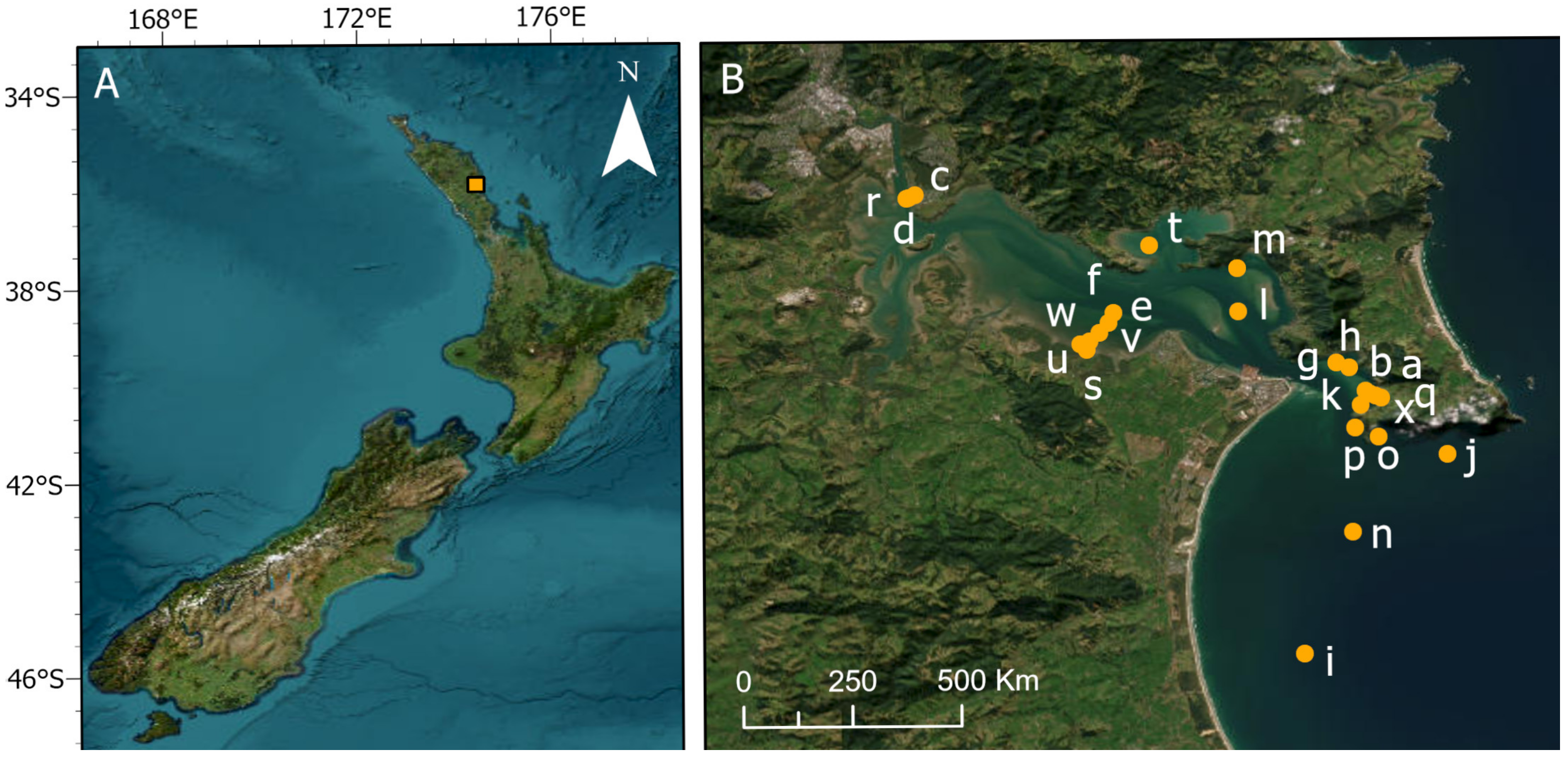
2.1. Study Area and Sampling

Twenty-four benthic sites were sampled in Whangārei Harbour and adjacent Bream Bay on the North Island of New Zealand (Figure 1).
Sampling was conducted during austral summer over 2 years, with 10 sites sampled in December 2019 and 14 sites in November 2020. At each site we videoed the seafloor to characterise habitat type and collected sediment cores to quantify benthic biodiversity and sediment characteristics (grain size, mud content, organic content and chlorophyll-a concentration). Either n = 3 or n = 10 large cores of sediment (13 cm internal diameter, 15 cm deep, area of 133 cm2) were collected for subsequent identification and enumeration of all sediment-associated invertebrates >500 µm (hereafter macrofauna). All macrofauna cores were sieved on a 500 µm mesh screen in the field before preservation in 70% Isopropyl alcohol. Five smaller cores of surficial sediment (2 cm internal diameter, 2 cm deep, area of 3.14 cm2) were collected and amalgamated (n = 1 per site) for later determination of sediment mud content (%), organic matter content (%) and chlorophyll-a concentration (µg/g dry weight of sediment). Sediment samples were frozen and stored in the dark until analysis.
Sediment samples for macrofauna were sorted, macrofauna identified to the lowest possible taxonomic level and counted. Sediment samples were analysed for particle size distribution, organic matter content, and chlorophyll-a concentration using previously published standard methods, e.g., [38]. Sediment particle size distribution was assessed by digesting a homogenised subsample in ~9% hydrogen peroxide, wet-sieving samples through 2000, 500, 250, and 63 μm mesh sieves, and measuring the dry weights of each fraction. Sediment organic matter content was determined as percentage dry weight lost following ignition in a 400 °C muffle furnace. For sediment chlorophyll-a content, a subsample of sediment was freeze dried, weighed, and homogenised before boiling in 90% ethanol. Concentrations of pigments in the ethanol extract were determined spectrophotometrically, with an acidification step used to distinguish chlorophyll-a from its degradation product, phaeophytin.
Each site was categorised according to habitat type, sediment mud content and water column depth (Table 1). Habitat at each site was determined following analysis of video collected by divers along a single 25 m transect per site (width of view ~70 cm; camera ~1 m above the seafloor). Structural features on the seafloor included physical characteristics and densities of habitat forming organisms, which were quantified during video analysis and the dominant habitat type determined at each site. Six broad habitat types were identified in this study: “seagrass”, shell hash dominated (hereafter “shelly”), polychaete worm tube mats (hereafter “tube mat”), “small burrows”, “large burrows”, and coarse sand with limited visible epifauna, dominated by infaunal molluscs Austrovenus stutchburyi and Notoacmea scapha (hereafter “infaunal molluscs”).
Sediment mud content categories were based on thresholds reported in the literature, e.g., [39,40,41,42,43]. Muddiness categories were defined as follows: 0–3%, 3–10%, 10–30%, >35% mud content. The mud content categories represented increasing levels of stress, based on a wealth of New Zealand literature documenting the deleterious effects of high bed sediment mud content on macrofauna abundance, diversity and functions, e.g., [33,44,45].
Water depth categories were defined so that there was a similar number of sites in each category (minimum of n = 3 sites per depth band). Intertidal sites were given a depth of 0 m and the six depth groupings were 0 m, 1–3 m, 3–6 m, 6–10 m, 10–15 m and 15–22 m. No values were on the group boundaries (e.g., 3, 6, 10 and 15 m, and 3 and 10% muddiness). Seabed depths were recorded by divers while on site and later adjusted according to tide height at the time of sampling (tidal range in Whangārei Harbour is ~2.3 m during a mean spring tide). Considering the significant influence of sediment mud content on estuarine biodiversity, the three sites within the highest mud grouping (>35%) were removed from all depth categories to deconfound the role of mud when investigating depth.
Although a key objective of the analysis was to determine the roles of biotic habitat type, mud content category, and depth zone on species richness, accumulation pattern, and functional redundancy (see below), the three types of categories created were not entirely independent. For example, none of the deepest sites were muddy, all of the intertidal sites were the same habitat type (infaunal molluscs) and all of the 1–3 m depth category were seagrass. In addition, the muddiest sites were between 1–6 m depth, and all of the muddiest sites made up the large burrows habitat group (see Figure S1 for a map of the locations of sites with each category grouping).

2.2. Data Analysis

To visualise the macrofaunal communities within and between sites, a non-metric multidimensional scaling (nMDS) of distances among centroids based on Bray–Curtis resemblance matrices (square root transformed) was conducted. Normalised and transformed environmental variables (depth, mud content, phaeophytin concentration and chlorophyll-a) which have the potential to covary with macrofaunal community structure were overlaid.
A combination of diversity metrics and analyses were used to describe the complexity of macrofauna community structure and composition. Accumulation curves were used to determine taxonomic richness within each category group as a function of sampling effort, using an approach similar to Ugland et al. [46]. The diversity of each group as a whole (γ-diversity) was determined from the richness predicted from an accumulation curve based on 16 cores. Sixteen cores was chosen as it represents the highest number of cores within all groups, and thus allowed for comparisons of γ-diversity among groups given a standardised sampling effort. Local α-diversity was defined as the average species richness within each group. Numerous measures of β-diversity have been reported in the literature, however, we calculated additive β-diversity, defined as γ-α diversity. Thus, we subtracted the average α-diversity of each group from the γ-diversity of that group. Additive β-diversity (rather than γ/α) was used as it more accurately describes heterogeneity from local to larger scales and connectivity between sites, rather than species turnover [47,48,49]. Species evenness (Pielou’s evenness), Shannon-Weiner and Simpson’s diversity indices were also calculated. A Kruskal–Wallis test followed by a Dunn’s test was performed for diversity indices where appropriate to identify any significant differences between groups.
To investigate the dissimilarity of species composition between groups, two approaches were used which focused on the species present/absent. The first involved multiple iterations of species accumulation curve building, where groups were combined in specific orders and new species accumulation curves were generated following each new addition to show the contribution of individual groups (habitat types, mud categories, depth zones) to total species pool richness. Mud and depth groups were combined in ascending order first (from lowest to highest mud, and from shallowest to deepest, respectively) and then descending order. Habitat types (which cannot be ordered numerically) were added in the order of increasing then decreasing average α-diversity. The second method used to analyse dissimilarity in species community composition between groups involved calculations of Jaccard’s dissimilarity index. This method was applied to each group based on average (across all replicated cores in a grouping) species composition. The resulting index enables a comparison of community composition by determining what percent of species identified were present in both populations, and thus provides a ratio of how similar (close to 0) or dissimilar (close to 1) a community is.
To assess functional redundancy, a Trait-Based Index (TBI) developed for New Zealand soft-sediment macrofauna was calculated at each site as detailed by Rodil et al. [50]. This index is derived from species richness within functional groups and therefore provides an assessment that is closely related to functional redundancy. TBI scores are based on the richness of species in seven particular trait modalities that were selected for their sensitivity to sediment muddiness and heavy metal contamination [50], the primary stressors influencing macrofaunal communities within New Zealand [51,52,53]: a living position in the top 2 cm, having an erect tube or structure, a mover of sediment from surface to surface (not vertically), sedentary, suspension feeding, worm shaped, of medium body size. The functional traits of all species present at each site were assigned using a collaboratively developed functional traits database held by the National Institute of Water & Atmospheric research (NIWA, New Zealand). Higher TBI index scores indicate higher functional redundancy (i.e., higher richness within the seven trait modalities). The relationship between TBI score and sediment mud content and water column depth were investigated using bivariate scatter plots with a regression line fitted based on lowest Akaike Information Criterion (AIC) value of separate polynomial models up to the 4th degree (Table S1). This allowed the assessment of both linear and curvilinear relationships. A multiple regression was then performed including both mud and depth using best fit procedure to investigate the combined contribution of mud and depth in explaining the variability of TBI score between sites.

3. Results

3.1. Estuary Characterisation and Group Selection

An nMDS ordination (Figure 2) of macrofaunal community data collected in the Whangārei/Bream Bay system showed replicates from individual sites clustering relatively close together, suggesting less variability within sites than among sites. Overlaid environmental vectors highlight the influence of water column depth and sediment mud content in driving the variability among sites. The individual species driving these differences between groups can be found in Table S2. For example, Micromaldane sp. was the most highly abundant taxa in the small burrows and tube mat habitat types, but was absent from all other habitats. In addition, the intertidal group was dominated by the amphipod family Lysianassidae and two mollusc species, Austrovenus stutchburyi and Notoacmea scapha which were absent in the subtidal groups.

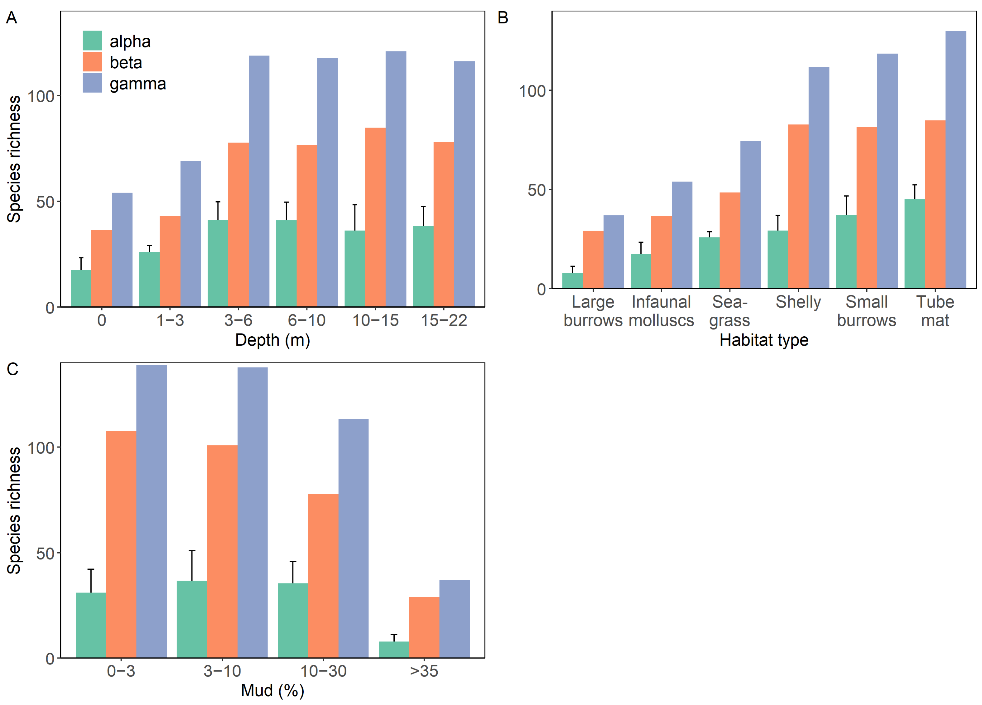
3.2. Patterns of Diversity within Groups

α- diversity was highly variable between groupings and ranged from an average of 8 to 45 species per group (Figure 3). α-, β- and γ- diversity increased with increasing depth up until 3–6 m, after which all values stabilised (Figure 3). Reductions in β- and γ- diversity were observed in communities with >10% mud, and >30% mud for α-diversity. When comparing habitat types, the lowest within-habitat α-, β- and γ-diversity values were observed within large burrow and then infaunal molluscs habitats, with all indices increasing across seagrass, shelly, small burrow and then tube mat habitats.
These patterns of diversity were reflected when comparing three different diversity indices (Shannon-Weiner diversity, Simpson’s diversity and Pielou’s evenness index (Figure S2)). Significantly lower Shannon diversity was observed within intertidal communities compared to all other depth groups (Kruskal–Wallis test, p < 0.001; Table S3), however, few differences were observed when using Simpson’s diversity. Pielou’s index suggests a slightly higher degree of evenness in the intertidal and lower subtidal habitats. Sediment mud content was strongly related to community diversity, whereby significantly lower Simpson and Shannon diversity values were observed in communities with >35% mud compared to all other groupings (Kruskal–Wallis test, Simpson diversity p < 0.001; Shannon diversity p < 0.001; Table S3). Additionally, communities of 10–30% mud had lower Simpson diversity than those with <10% mud, but Shannon diversity and evenness were comparable (Table S3). Between habitat types, the composition of the large burrows group containing only sites with >35% mud resulted in this group having significantly lower diversity than all other habitat types (Table S3). Infaunal molluscs habitats were the only other habitat type to have significantly lower Shannon diversity when compared to almost all other groups (except tube mats).

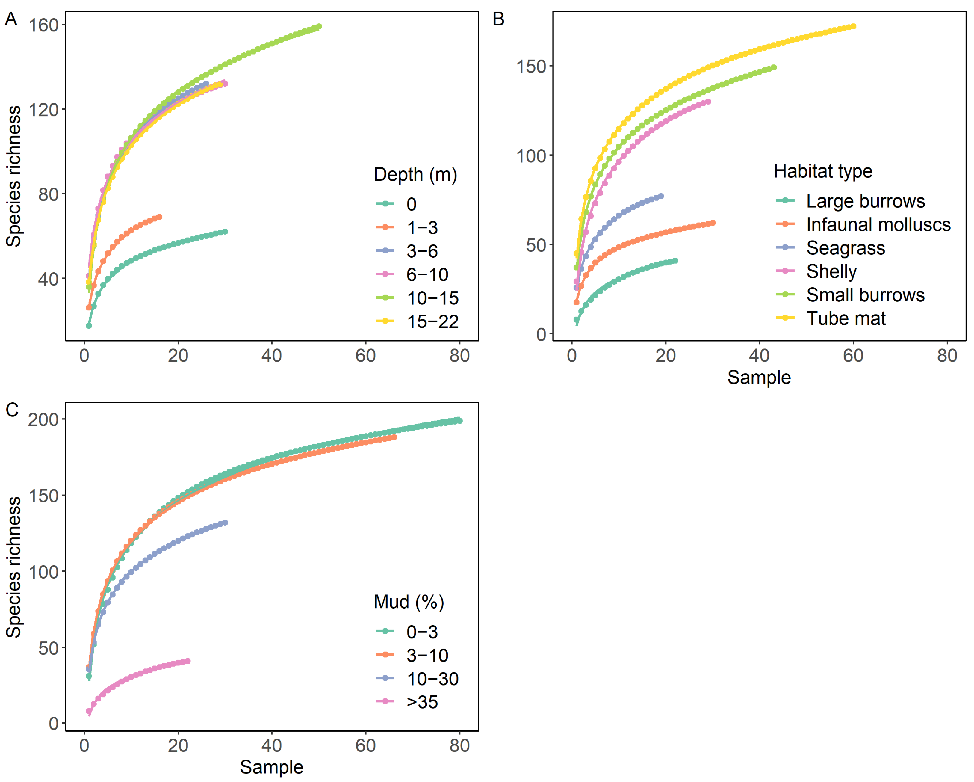
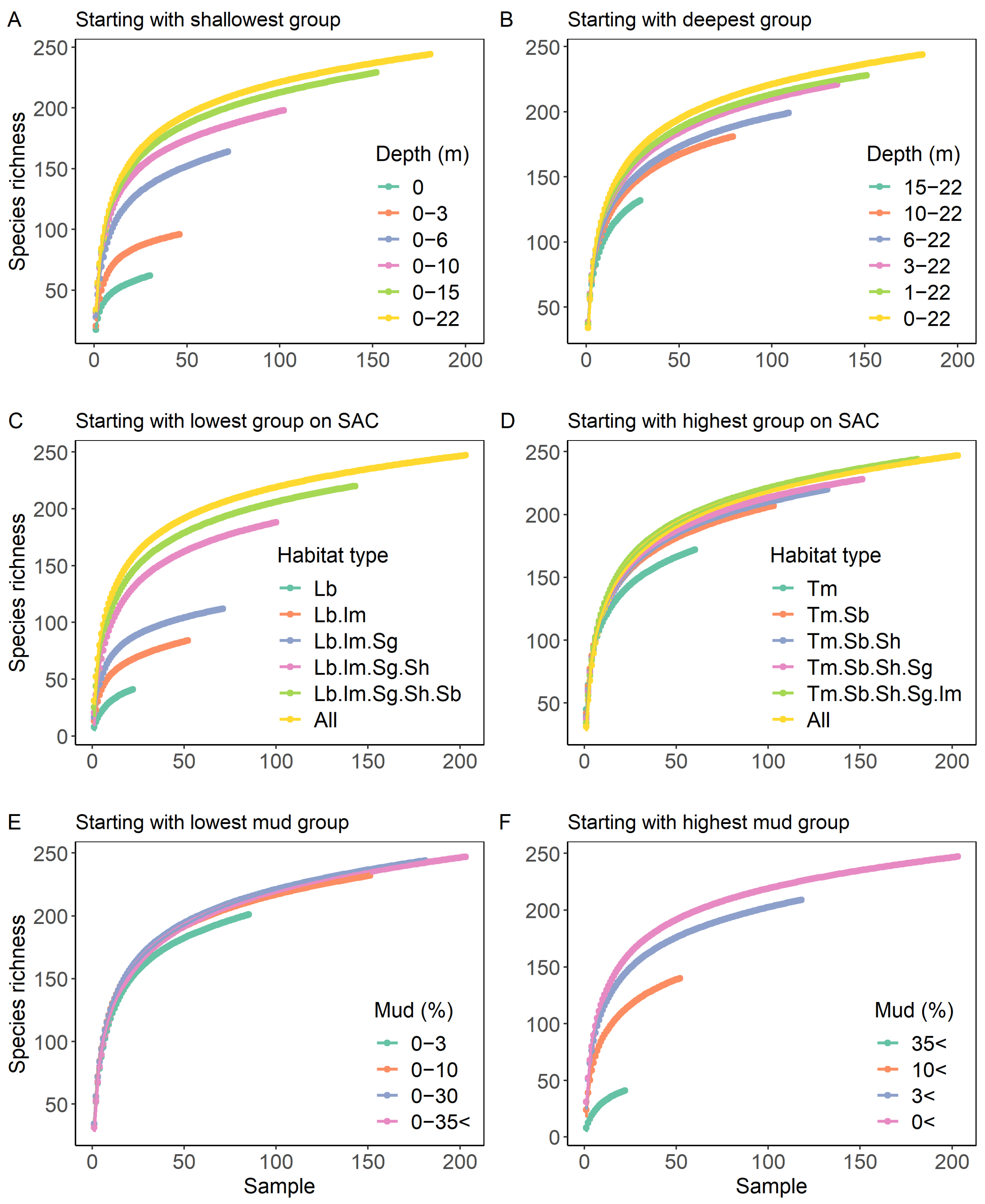
3.3. Species Accumulation in Relation to Sediment Mud Content, Water Column Depth and Habitat Type

Species accumulation curves highlight the differences in species richness among groups relative to sampling effort (Figure 4). When standardised by sampling effort, species richness was similar in the two lowest mud content categories (0–3 and 3–10% mud) but decreased by 19% and 73% when mud content increased to 10–30% and >35%, respectively. Species richness for subtidal communities deeper than 3 m were relatively indistinguishable from each other and did not reach an asymptote within the sampling range (up to 50 replicate samples). However, species richness was considerably lower at a depth of 1–3 m (−41%) and for intertidal communities (−54%). Species richness varied by habitat type, with a 71% difference between the lowest and highest species richness for a given sampling effort. The lowest richness was observed in large burrow, followed by infaunal molluscs and seagrass habitats, whilst the other three habitat types had considerably higher species richness.

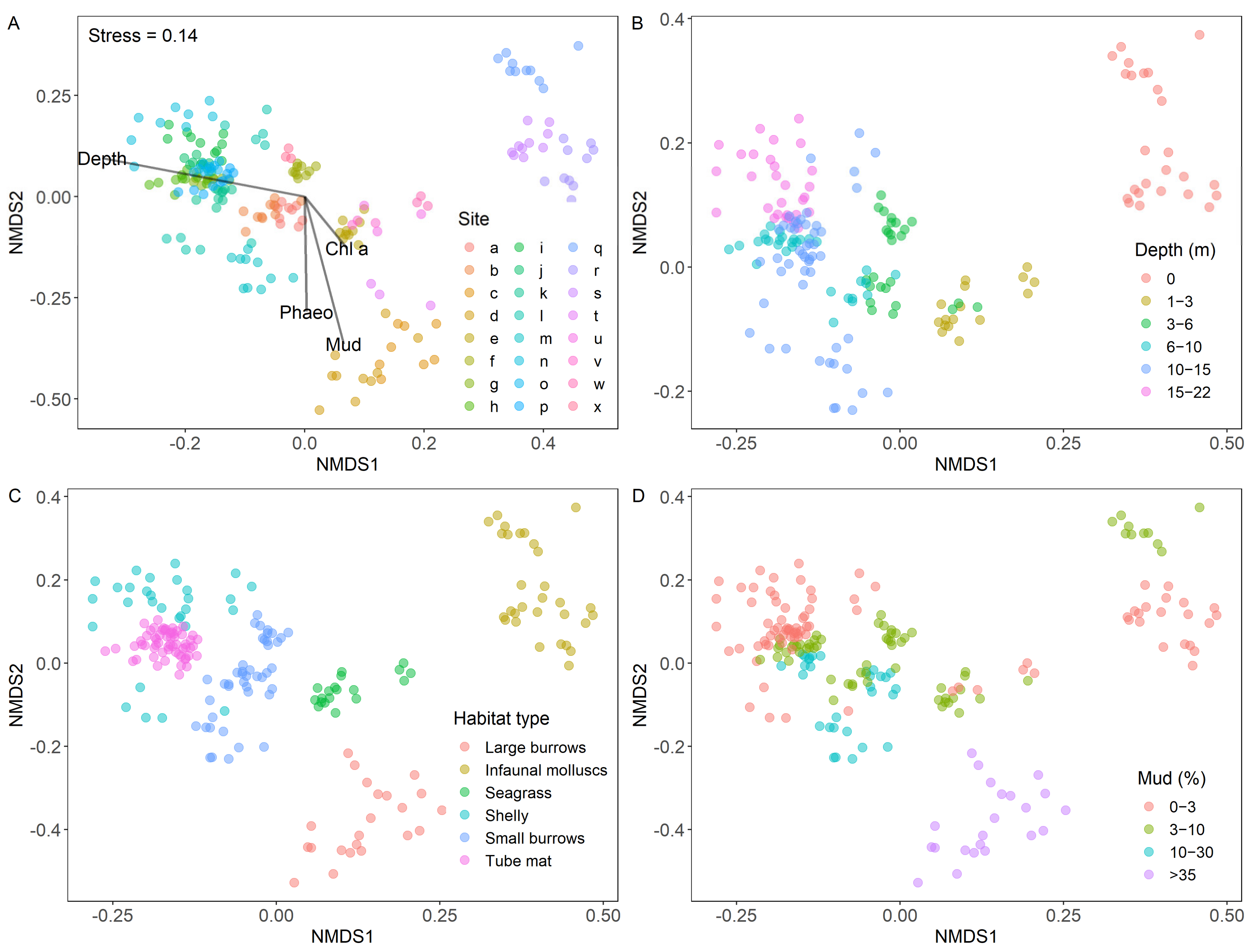
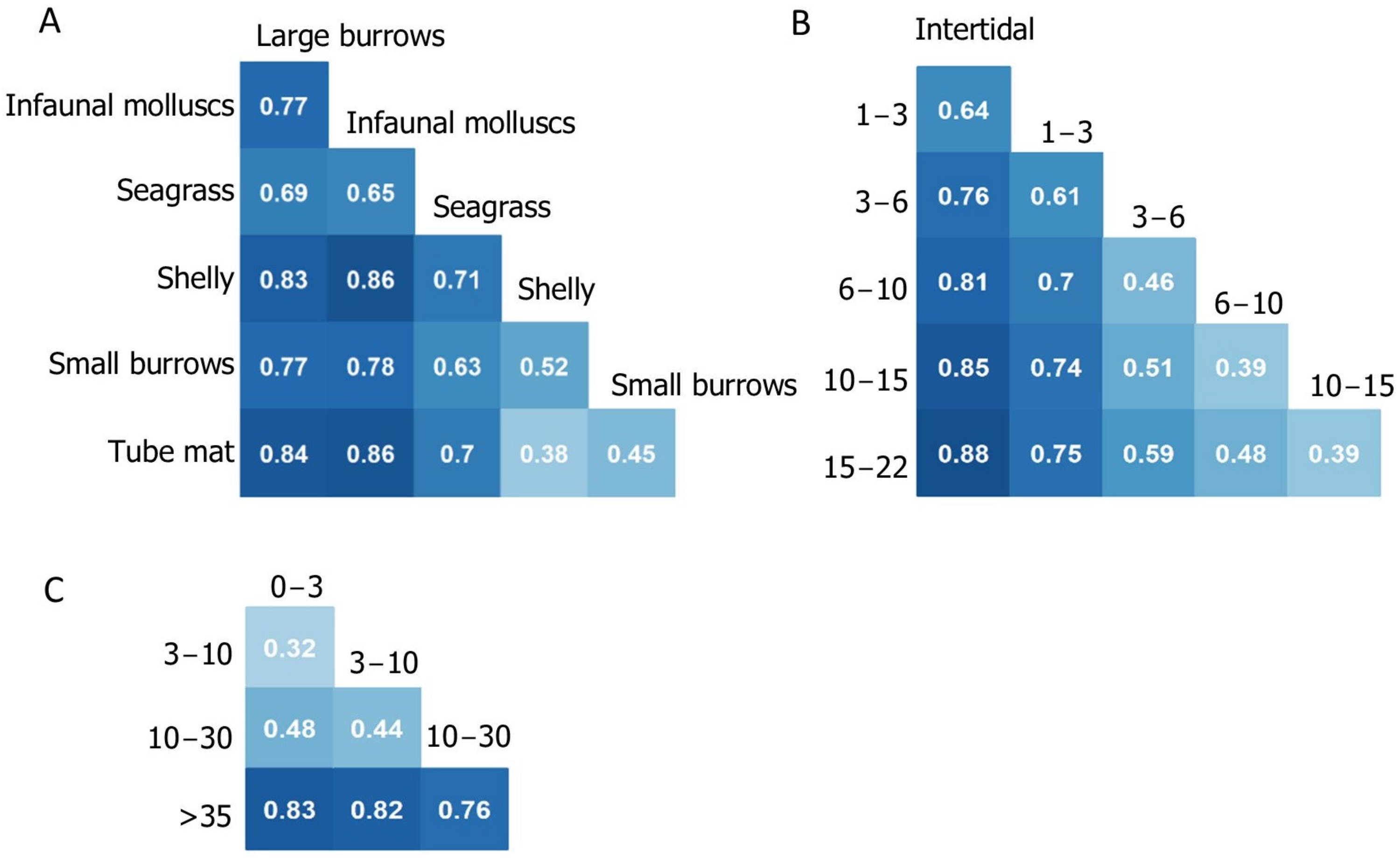
3.4. Dissimilarity Patterns within Groups

Whilst species richness may be similar among sites and groups for a given sampling effort, community composition (i.e., the particular species present) can differ widely (i.e., there can be turnover) (Table S2).

3.4.1. Water Column Depth

In Figure 5A, the first group plotted was the 0 m depth group (intertidal), followed by the 0 and 1–3 m depth groups combined (i.e., a 0–3 m grouping). The large difference between the first two curves of Figure 5A (0 m and 0–3 m) indicated that many new species contributed to the increased species richness. Conversely, when the last depth group was added (adding the 15–22 m group to produce a 0–22 m curve), a relatively small increase in species richness resulted. Thus, the species occurring within this group were mostly a subset of those found in the remaining groups. On the other hand, when starting with the deepest depth group (Figure 5B), increases in species richness were less pronounced, with the majority of species included within the two deepest depth groups. These relationships were reflected in the calculation of Jaccard’s dissimilarity index (Figure 6). The lowest dissimilarity (<50%) was observed between the deeper subtidal groups (>3 m) and dissimilarity in species composition was lowest in adjacent groups. For example, intertidal communities had the highest similarity to 1–3 m depth, with dissimilarity increasing with increasing depth.

3.4.2. Habitat Type

Similar to the patterns observed with depth, when starting with the habitat type with the highest species richness (analogous to starting with the deepest group, Figure 5D), few new species were added when including additional habitat groups. Conversely, when starting with “large burrows”, the habitat type with the lowest species richness, new species were added with each additional habitat group (Figure 5C). The majority of habitat groups showed high dissimilarity to each other, with an average dissimilarity of 70% across all habitat groups. Dissimilarity was highest for the least diverse groups: large burrows and infaunal molluscs habitats.

3.4.3. Sediment Mud Content

When comparing species richness within the sediment mud content groups, almost all species occurred in the two groups with the least mud (0–3% and 3–10%; Figure 5E). Few new species occurred within the highest mud groups (10–30% mud and >35% mud). In contrast, when starting with the highest mud group (which was relatively species poor; Figure 5F), large increases in richness occurred when sites with less mud were incorporated into the groupings. Jaccard’s dissimilarity index supports the considerable difference in species composition between >35% mud and all other groups, with dissimilarity ranging between 76–83%. The lowest dissimilarity occurred between the 0–3 and 3–10% mud categories, which increased with increasing mud content.

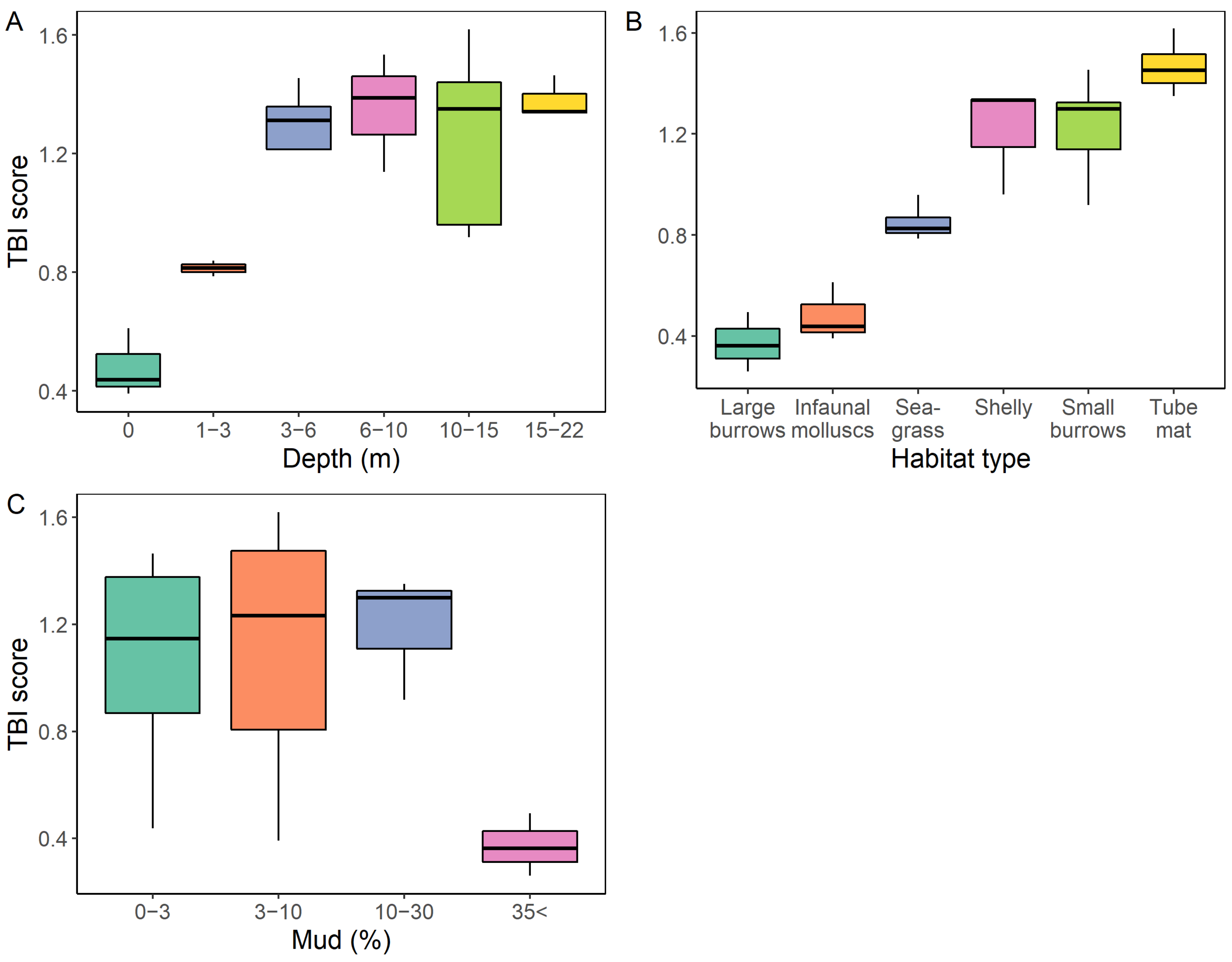
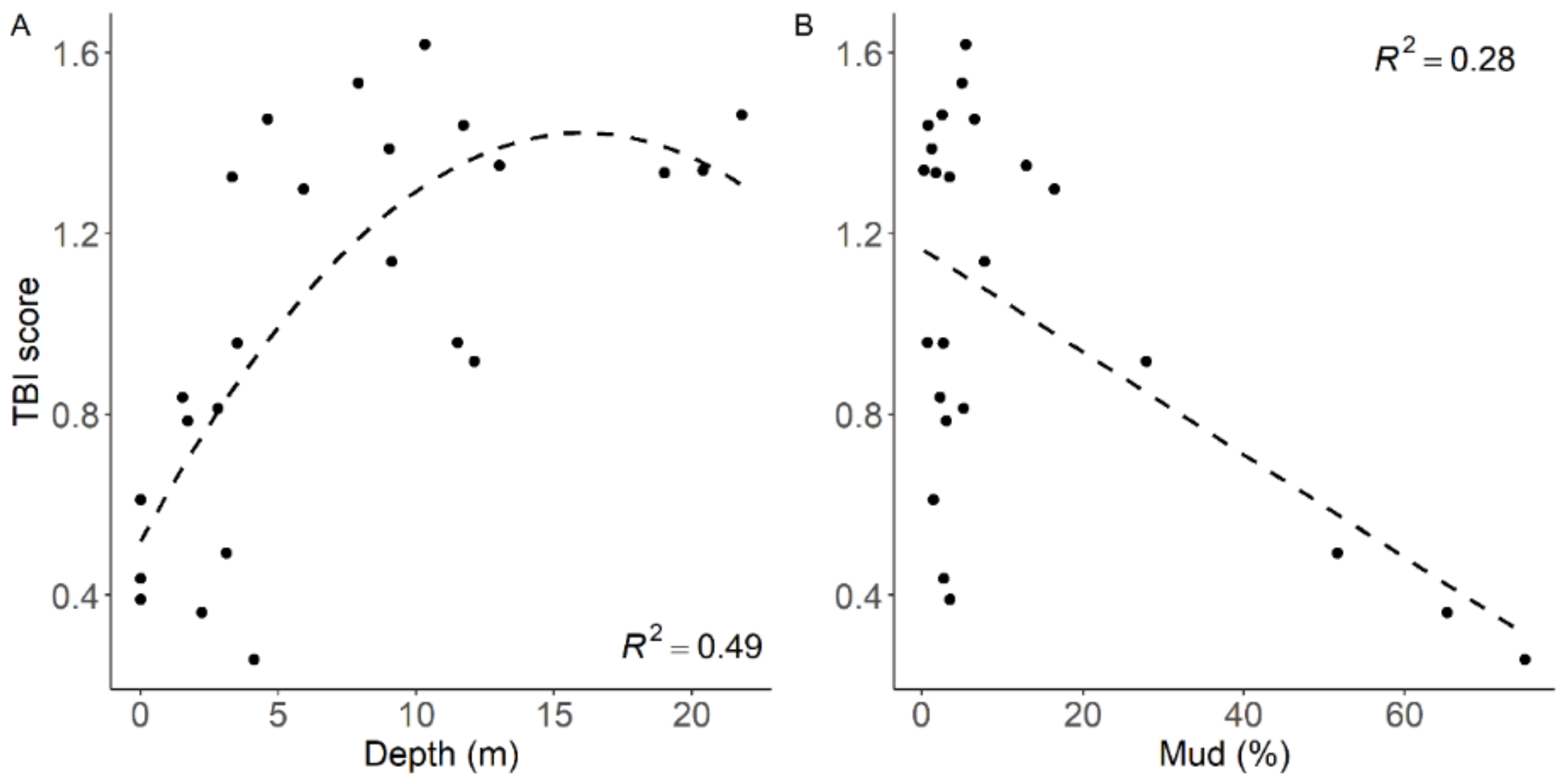
3.5. Changes in Functional Redundancy between Groups

TBI scores ranged between 0.26 and 1.62, with 50% of scores over 1, and 88% of scores over 0.4 (Figure 7). Sites with the lowest functional redundancy index values were observed at sites with >35% mud and in the shallower parts of the estuary (intertidal and 1–3 m depth groupings), which were categorised as infaunal molluscs and large burrow habitats (Figure 7).
TBI scores were originally developed in relation to species responsiveness to gradients of mud and heavy metal concentration in intertidal areas. Across sites in Whangārei Harbour, sediment mud content was inversely correlated to TBI score, but there was high variability when mud content was below 3% (Figure 8). This resulted in maximal TBI scores at ~5% mud, before a strong decrease and thus the lowest calculated TBI scores when sediment mud content was high (>60%). TBI scores were low in the intertidal zone and at depths <3 m, increasing to maximal TBI scores when depth was between 4–12 m, before decreasing at depths greater than 15 m. Combined, sediment mud content and water column depth explained 56% of the variability in TBI score between sites.

4. Discussion

This study highlights the high heterogeneity of macrofauna communities that can occur within estuarine ecosystems and the influence of different environmental gradients in determining species richness and functional redundancy, which provide insights into resilience and recovery responses. We observed strong gradients in biodiversity, with the highest biodiversity at sandier, deeper sites with more abundant macrofauna community structure. In contrast, the lowest biodiversity was observed at muddy, intertidal and shallow subtidal sites, which were dominated by large burrows and low abundances of macrofauna. As biodiversity is a key contributor to ecosystem resilience, these results suggest that the impact of future stressors such as sea level rise or increased sedimentation are likely to be highly spatially variable across different estuarine habitat types. In addition, our research indicates that a comparative lack of subtidal sampling within estuaries may be resulting in assessments of vulnerability to future change inadequately protecting high value subtidal habitats. This is particularly the case where estuarine monitoring programmes (such as those within New Zealand) focus primarily on intertidal habitats and thus may be substantially underestimating biodiversity and functional redundancy within these areas. Moreover, the high biodiversity observed within the subtidal habitats of this study suggested these areas may contribute the most to the overall species pool, indicative of their potential importance to disturbance recovery dynamics.
A strong driver of biodiversity in our study was sediment mud content, with increased muddiness (particularly >35%) resulting in a reduction of all measures of biodiversity, in agreement with previous research, e.g., [33,34,35,44]. For example, Shannon and Simpson diversity indices were significantly lower for sites with >35% mud, and when compared to 0–10% mud, γ-diversity decreased by 19% and 73% for mud content between 10–30% and >35%, respectively. Low γ- and β- diversity as observed in the >35% group has previously been suggested to indicate these areas are highly degraded [18]. Furthermore, iteratively combining species accumulation curves showed there were few new species present at sites with >35% mud when compared to all other mud groups. This suggests species within the high mud group were a small subset of those found within the wider community, resulting in less diverse communities dominated by a small number of species that were tolerant of high mud content.
Increased muddiness is often a consequence of hydrodynamic conditions, with quiescent areas of low flow predisposed to increased accumulations of fine sediments. Eroded soil (terrigenous sediment) is considered to be one of key contaminants affecting New Zealand’s estuaries, with an estimated 192 million tonnes of soil being lost from the land each year [54]. Over time, as sediment accumulates in estuaries it can result in changes to the cohesiveness of surface sediment, inhibit diffusive and advective transport of solutes resulting in changes to porewater geochemistry, alter food quality through nutritional differences of terrestrial and marine sediments, block filter-feeding appendages, and deter larval settlement [44,45,55]. The resulting changes to community composition have direct effects on ecosystem functioning such that high mud regions have been shown to have reduced nutrient processing capacity (including denitrification) and benthic primary productivity [34,35,36,56].
Whilst the relationship between biodiversity and mud is relatively well established, fewer comparisons exist between biodiversity and water column depth, with the majority of studies focusing on either intertidal or subtidal areas separately. However, within this study, water column depth had a significant influence on community composition and biodiversity, as highlighted by 88% maximum dissimilarity of species composition between depth groups (Figure 6). Differences were greater within intertidal and shallow subtidal regions (0 and 1–3 m), resulting in significantly lower α-, β- and γ- diversity values, which were comparable to those found in intertidal areas elsewhere [24]. However, shallower depth groups had higher evenness (Pielou’s index) than those >3 m and showed considerable overlap in species composition (Figure 5), suggesting the potential loss of several highly abundant species which were less tolerant to shallow subtidal and intertidal conditions (e.g., differential flow rates, oscillating emerged periods) such as the polychaete tube mats found only at depths >6 m. Differences in hydrodynamic conditions have previously been associated with changes in biodiversity within intertidal areas globally [57], and have been attributed to intertidal extent negatively affecting biodiversity [24]. This can be a consequence of high wave-exposure and changes in current patterns influencing erosion rates and the dispersal of organisms [58,59]. While the inclusion of only one habitat within the intertidal depth group within this study restricts the ability to make generalisations over varied intertidal areas and to comprehensively compare subtidal and intertidal biodiversity, the comparable biodiversity estimates to those across a number of other intertidal habitats and estuaries [24] suggests the intertidal area within this study is likely to be representative of those found elsewhere.
The strong influence of both sediment mud content and water column depth on the biota was also evident within the habitat groupings. For example, the “large burrows” habitat category occurred exclusively at high mud sites (>35%), the “infaunal molluscs” habitat was restricted to the intertidal zone (0 m group), and the majority of seagrass sites (3 out of 4) were present in the 1–3 m depth grouping. Consequently, these three habitat types had the lowest biodiversity. Within mud and sand habitats, the absence or low abundances of habitat formers can result in a homogenous sediment that lacks 3-dimensional complexity and thus can have lower α-diversity than other habitats [57,60]. Conversely, polychaete tube mat habitats, for example, can increase sediment deposition (including organic matter) which can enhance sediment stability and facilitate deposit feeders [61,62,63]. Reduced structural complexity is also likely to have influenced the seagrass habitat because of the sparse growth form and relatively short blades of the species that grows within New Zealand (Zostera mulleri) [24,64] and the infauna mollusc group which had variable abundances of the cockle Austrovenus stutchburyi.
Analysis of functional groups is frequently used to provide more information on the consequences of species loss than overall taxonomic richness [65,66]. In this study, sites with lower sediment mud content had much higher TBI scores indicating greater functional redundancy (e.g., 1.0 for <3% mud vs. 0.37 for the >35% mud), however there was significant variation around very low mud sites (<3% mud). The high variance around sites with <3% mud and the relationship between sediment mud content and TBI scores observed in Whangārei Harbour (r2 = 0.28) was similar to that observed previously (negative trend, r2 = 0.36, across other North Island sites; [50]). The former was attributed to differences in hydrodynamic conditions, such as high wind and wave activity resuspending fine sediments (mud) resulting in unstable and poor-quality food availability rather than a response to anthropogenic impacts. However, it should be noted that TBI scores were much higher overall in this study relative to the more urbanised and human-affected estuaries of the Auckland Region where the TBI index was developed, where >0.4 is considered a high TBI score.
More influential than sediment mud content, this study showed a stronger relationship of TBI score with water column depth (r2 = 0.49), the first use of the index in this way. Combined with sediment mud content, 56% of the variability in TBI score was explained, highlighting the dominance of these two gradients in influencing community composition. It should, however, be noted that only a small number of intertidal sites were included within this study, restricting intertidal versus subtidal comparisons. Nonetheless, TBI score increased with depth up to ~15 m whereby it plateaued, most likely a consequence of the similarity in community composition between the deeper subtidal sites (39% dissimilarity). Consequently, intertidal and shallow subtidal regions were estimated to have lower functional redundancy and are therefore suggested to be more susceptible to new or increased stressors. Whilst this would imply these communities are unable to cope with further stress and thus the effects of new stressors are amplified, e.g., [7,8], it has also been argued that these communities may alternatively be adapted to stress and therefore the response to further stressors may instead be lessened [9,10,11]. Discerning how emerging stressors will interact with current environmental pressures and gradients is therefore essential when trying to predict community responses to future change.
Sea-level rise is already impacting coastal areas globally, and whilst the magnitude is uncertain, it will likely create new pressures on benthic fauna through the deepening of subtidal areas which will shift or squeeze intertidal areas [67]. Within this study we observed significant changes in estuarine biodiversity along a gradient of water column depth highlighting the need to quantify what exists subtidally in order to understand the vulnerability of estuaries to future change. Increases in subtidal habitats have the potential to provide the opportunity for biodiversity enhancement due to increased surface area of highly biodiverse subtidal regions, such as those reported within this study. However, sea-level rise will co-occur with changes in hydrodynamic conditions as well as increases in rainfall, suggesting sedimentation may intensify in the future resulting in increased turbidity and the deposition of sediment [68]. For some habitats, the interaction between these two stressors may inhibit the potential for biodiversity enhancement. For example, seagrass beds are highly sensitive to water column turbidity and sedimentation [69], therefore, sea-level rise would restrict the emerged periods currently providing a refuge from this temporal stressor and thus reduce the viability of these important habitats [70]. Understanding the differences in biodiversity and functionality between intertidal and subtidal areas is fundamental to informing management decisions in order to better facilitate these transitions.
Low diversity areas in Whangārei Harbour including intertidal habitats and sites with >35% mud may be areas of higher ecological stress where only relatively stress-tolerant species survive. Species living in permanently submerged, deeper areas would be less likely to experience thermal extremes, desiccation, and physical disturbance by waves, and therefore may be less resilient to future change than habitats which have adapted or been degraded due to higher stress. Similarly, muddy sites are generally associated with high stress in the form of high suspended sediment concentrations, high rates of sediment deposition, lower levels of sediment oxygenation, and higher concentrations of ammonium and sulphides, e.g., [32,33]. Our analysis suggests the species present in muddy and intertidal sites were a subset of the species present in adjacent sandier and deeper habitats in Whangārei, which likely increases their resilience (via connectivity) and improves their chances for recovery when disturbed (if the stressor is displaced). Our study highlights the importance of studying the individual contributions of different habitats in a landscape to characterise effective colonist pool size and how this can be used to predict recovery potential at disturbed sites.

Supplementary Materials

The following supporting information can be downloaded at: https://www.mdpi.com/article/10.3390/d14110998/s1, Figure S1: Locations of the sampling sites as a function of grouping; Figure S2: Pielous’ evenness, Simpson index and Shannon Wiener diversity indices by group; Table S1: AIC values of the regression models; Table S2: Ten of the most highly abundant taxa per group; Table S3: Results of the Kruskal–Wallis tests.

Author Contributions

Conceptualization, S.M., A.M.L., J.E.H. and R.H.B.; methodology, S.M., A.M.L., J.E.H. and R.H.B.; formal analysis, S.M.; investigation, A.M.L., B.L.G., S.F.H., K.C. and R.H.B.; data curation, R.H.B., B.L.G., S.F.H. and K.C.; writing—original draft preparation, S.M.; writing—review and editing, S.M., A.M.L., B.L.G., S.F.H., K.C., J.E.H. and R.H.B.; visualization, S.M.; supervision, A.M.L. and R.H.B.; project administration, A.M.L. and R.H.B.; funding acquisition, A.M.L. All authors have read and agreed to the published version of the manuscript.

Funding

This research was supported by the New Zealand Government’s Strategic Science Investment Fund (SSIF) to the National Institute for Water & Atmospheric Research (NIWA) and the Sustainable Seas National Science Challenge (CO1X1515).

Institutional Review Board Statement

Not applicable.

Data Availability Statement

The data presented in this study are available on request from the corresponding author.

Acknowledgments

Special thanks to Patuharakeke for co-developing the research with us and to Taryn Shirkey specifically who participated in field work. We acknowledge the Marine Ecology team at NIWA for assistance with sample processing and Jack Massuger and Fabrice Stephenson for diving/boating support. We also thank two anonymous reviewers for constructive comments on the manuscript.

Conflicts of Interest

The authors declare no conflict of interest. The funders had no role in the design of the study; in the collection, analyses, or interpretation of data; in the writing of the manuscript; or in the decision to publish the results.

References

  1. Hughes, T.P.; Bellwood, D.R.; Folke, C.; Steneck, R.S.; Wilson, J. New paradigms for supporting the resilience of marine ecosystems. Trends Ecol. Evol. 2005, 20, 380–386. [Google Scholar] [CrossRef] [PubMed]
  2. Palumbi, S.R.; McLeod, K.L.; Grünbaum, D. Ecosystems in Action: Lessons from Marine Ecology about Recovery, Resistance, and Reversibility. BioScience 2008, 58, 33–42. [Google Scholar] [CrossRef]
  3. Oliver, T.H.; Heard, M.S.; Isaac, N.J.B.; Roy, D.B.; Procter, D.; Eigenbrod, F.; Freckleton, R.; Hector, A.; Orme, C.D.L.; Petchey, O.L.; et al. A Synthesis is Emerging between Biodiversity-Ecosystem Function and Ecological Resilience Research: Reply to Mori. Trends Ecol. Evol. 2016, 31, 89–92. [Google Scholar] [CrossRef] [PubMed] [Green Version]
  4. Oliver, T.H.; Heard, M.S.; Isaac, N.J.B.; Roy, D.B.; Procter, D.; Eigenbrod, F.; Freckleton, R.; Hector, A.; Orme, C.D.L.; Petchey, O.L.; et al. Biodiversity and Resilience of Ecosystem Functions. Trends Ecol. Evol. 2015, 30, 673–684. [Google Scholar] [CrossRef] [PubMed] [Green Version]
  5. Walker, B.H. Biodiversity and Ecological Redundancy. Conserv. Biol. 1992, 6, 18–23. [Google Scholar] [CrossRef]
  6. Gamfeldt, L.; Lefcheck, J.S.; Byrnes, J.E.K.; Cardinale, B.J.; Duffy, J.E.; Griffin, J.N. Marine biodiversity and ecosystem functioning: What’s known and what’s next? Oikos 2015, 124, 252–265. [Google Scholar] [CrossRef] [Green Version]
  7. Albright, R.; Mason, B. Projected Near-Future Levels of Temperature and pCO2 Reduce Coral Fertilization Success. PLoS ONE 2013, 8, e56468. [Google Scholar] [CrossRef] [Green Version]
  8. Lenihan, H.S.; Micheli, F.; Shelton, S.W.; Peterson, C.H. The influence of multiple environmental stressors on susceptibility to parasites: An experimental determination with oysters. Limnol. Oceanogr. 1999, 44, 910–924. [Google Scholar] [CrossRef] [Green Version]
  9. Maltby, L. Studying stress: The importance of organism-level responses. Ecol. Appl. 1999, 9, 431–440. [Google Scholar] [CrossRef]
  10. Elliott, M.; Quintino, V. The Estuarine Quality Paradox, Environmental Homeostasis and the difficulty of detecting anthropogenic stress in naturally stressed areas. Mar. Pollut. Bull. 2007, 54, 640–645. [Google Scholar] [CrossRef]
  11. Rautenberger, R.; Bischof, K. Impact of temperature on UV-susceptibility of two Ulva (Chlorophyta) species from Antarctic and Subantarctic regions. Polar Biol. 2006, 29, 988–996. [Google Scholar] [CrossRef] [Green Version]
  12. Gladstone-Gallagher, R.V.; Pilditch, C.A.; Stephenson, F.; Thrush, S.F. Linking Traits across Ecological Scales Determines Functional Resilience. Trends Ecol. Evol. 2019, 34, 1080–1091. [Google Scholar] [CrossRef] [PubMed]
  13. Greenfield, B.L.; Kraan, C.; Pilditch, C.A.; Thrush, S.F. Mapping functional groups can provide insight into ecosystem functioning and potential resilience of intertidal sandflats. Mar. Ecol. Prog. Ser. 2016, 548, 1–10. [Google Scholar] [CrossRef] [Green Version]
  14. Loreau, M.; Mouquet, N.; Gonzalez, A. Biodiversity as spatial insurance in heterogeneous landscapes. Proc. Natl. Acad. Sci. USA 2003, 100, 12765–12770. [Google Scholar] [CrossRef] [Green Version]
  15. Tscharntke, T.; Tylianakis, J.M.; Rand, T.A.; Didham, R.K.; Fahrig, L.; Batáry, P.; Bengtsson, J.; Clough, Y.; Crist, T.O.; Dormann, C.F.; et al. Landscape moderation of biodiversity patterns and processes—Eight hypotheses. Biol. Rev. 2012, 87, 661–685. [Google Scholar] [CrossRef]
  16. Baselga, A. Partitioning the turnover and nestedness components of beta diversity. Glob. Ecol. Biogeogr. 2010, 19, 134–143. [Google Scholar] [CrossRef]
  17. Legendre, P. Interpreting the replacement and richness difference components of beta diversity. Glob. Ecol. Biogeogr. 2014, 23, 1324–1334. [Google Scholar] [CrossRef]
  18. De Juan, S.; Thrush, S.F.; Hewitt, J.E. Counting on β-Diversity to Safeguard the Resilience of Estuaries. PLoS ONE 2013, 8, e65575. [Google Scholar] [CrossRef]
  19. Hewitt, J.E.; Thrush, S.F.; Lohrer, A.M.; Townsend, M.J. A latent threat to biodiversity: Consequences of small-scale heterogeneity loss. Biodivers. Conserv. 2010, 19, 1315–1323. [Google Scholar] [CrossRef]
  20. Thrush, S.F.; Hewitt, J.E.; Cummings, V.J.; Norkko, A.; Chiantore, M. β-Diversity and Species Accumulation in Antarctic Coastal Benthos: Influence of Habitat, Distance and Productivity on Ecological Connectivity. PLoS ONE 2010, 5, e11899. [Google Scholar] [CrossRef]
  21. Telesh, I.V.; Khlebovich, V.V. Principal processes within the estuarine salinity gradient: A review. Mar. Pollut. Bull. 2010, 61, 149–155. [Google Scholar] [CrossRef] [PubMed]
  22. Van der Wal, D.; Lambert, G.I.; Ysebaert, T.; Plancke, Y.M.G.; Herman, P.M.J. Hydrodynamic conditioning of diversity and functional traits in subtidal estuarine macrozoobenthic communities. Estuar. Coast. Shelf Sci. 2017, 197, 80–92. [Google Scholar] [CrossRef] [Green Version]
  23. Zhu, C.; van Maren, D.S.; Guo, L.; Lin, J.; He, Q.; Wang, Z.B. Effects of Sediment-Induced Density Gradients on the Estuarine Turbidity Maximum in the Yangtze Estuary. J. Geophys. Res. Ocean. 2021, 126, e2020JC016927. [Google Scholar] [CrossRef]
  24. De Juan, S.; Hewitt, J. Relative importance of local biotic and environmental factors versus regional factors in driving macrobenthic species richness in intertidal areas. Mar. Ecol. Prog. Ser. 2011, 423, 117–129. [Google Scholar] [CrossRef] [Green Version]
  25. Lotze, H.K.; Lenihan, H.S.; Bourque, B.J.; Bradbury, R.H.; Cooke, R.G.; Kay, M.C.; Kidwell, S.M.; Kirby, M.X.; Peterson, C.H.; Jackson, J.B.C. Depletion, Degradation, and Recovery Potential of Estuaries and Coastal Seas. Science 2006, 312, 1806–1809. [Google Scholar] [CrossRef]
  26. McWethy, D.B.; Whitlock, C.; Wilmshurst, J.M.; McGlone, M.S.; Fromont, M.; Li, X.; Dieffenbacher-Krall, A.; Hobbs, W.O.; Fritz, S.C.; Cook, E.R. Rapid landscape transformation in South Island, New Zealand, following initial Polynesian settlement. Proc. Natl. Acad. Sci. USA 2010, 107, 21343–21348. [Google Scholar] [CrossRef] [Green Version]
  27. Abrahim, G.; Parker, R. Heavy-metal contaminants in Tamaki Estuary: Impact of city development and growth, Auckland, New Zealand. Environ. Geol. 2002, 42, 883–890. [Google Scholar] [CrossRef]
  28. Moller, H.; MacLeod, C.J.; Haggerty, J.; Rosin, C.; Blackwell, G.; Perley, C.; Meadows, S.; Weller, F.; Gradwohl, M. Intensification of New Zealand agriculture: Implications for biodiversity. N. Z. J. Agric. Res. 2008, 51, 253–263. [Google Scholar] [CrossRef] [Green Version]
  29. Swales, A.; Williamson, R.B.; Van Dam, L.F.; Stroud, M.J.; McGlone, M.S. Reconstruction of urban stormwater contamination of an estuary using catchment history and sediment profile dating. Estuaries 2002, 25, 43–56. [Google Scholar] [CrossRef]
  30. Hicks, D.M.; Shankar, U.; McKerchar, A.I.; Basher, L.; Lynn, I.; Page, M.; Jessen, M. Suspended sediment yields from New Zealand rivers. J. Hydrol. 2011, 50, 81–142. [Google Scholar]
  31. Thrush, S.F.; Hewitt, J.E.; Cummings, V.J.; Ellis, J.I.; Hatton, C.; Lohrer, A.; Norkko, A. Muddy Waters: Elevating Sediment Input to Coastal and Estuarine Habitats. Front. Ecol. Environ. 2004, 2, 299–306. [Google Scholar] [CrossRef]
  32. Cummings, V.; Vopel, K.; Thrush, S. Terrigenous deposits in coastal marine habitats: Influences on sediment geochemistry and behaviour of post-settlement bivalves. Mar. Ecol. Prog. Ser. 2009, 383, 173–185. [Google Scholar] [CrossRef]
  33. Lohrer, A.M.; Thrush, S.F.; Hewitt, J.E.; Berkenbusch, K.; Ahrens, M.; Cummings, V.J. Terrestrially derived sediment: Response of marine macrobenthic communities to thin terrigenous deposits. Mar. Ecol. Prog. Ser. 2004, 273, 121–138. [Google Scholar] [CrossRef] [Green Version]
  34. Pratt, D.R.; Lohrer, A.M.; Pilditch, C.A.; Thrush, S.F. Changes in Ecosystem Function Across Sedimentary Gradients in Estuaries. Ecosystems 2014, 17, 182–194. [Google Scholar] [CrossRef]
  35. Robertson, B.P.; Gardner, J.P.A.; Savage, C. Macrobenthic–mud relations strengthen the foundation for benthic index development: A case study from shallow, temperate New Zealand estuaries. Ecol. Indic. 2015, 58, 161–174. [Google Scholar] [CrossRef]
  36. Rodil, I.F.; Lohrer, A.M.; Chiaroni, L.D.; Hewitt, J.E.; Thrush, S.F. Disturbance of sandflats by thin terrigenous sediment deposits: Consequences for primary production and nutrient cycling. Ecol Appl 2011, 21, 416–426. [Google Scholar] [CrossRef]
  37. Swales, A.; Gibbs, M.; Pritchard, M.; Budd, R.; Olsen, G.; Ovenden, R.; Costley, K.; Hermanspahn, N.; Griffiths, R. Whangarei Harbour Sedimentation: Sediment Accumulation Rates and Present-Day Sediment Sources; National Institute of Water and Atmospheric Research: Auckland, New Zealand, 2013; p. 40. [Google Scholar]
  38. Bulmer, R.H.; Schwendenmann, L.; Lohrer, A.M.; Lundquist, C.J. Sediment carbon and nutrient fluxes from cleared and intact temperate mangrove ecosystems and adjacent sandflats. Sci. Total Environ. 2017, 599–600, 1874–1884. [Google Scholar] [CrossRef]
  39. Cummings, V.J.; Thrush, S.F. Behavioural response of juvenile bivalves to terrestrial sediment deposits: Implications for post-disturbance recolonisation. Mar. Ecol. Prog. Ser. 2004, 278, 179–191. [Google Scholar] [CrossRef] [Green Version]
  40. Hohaia, A.; Vopel, K.; Pilditch, C.A. Thin terrestrial sediment deposits on intertidal sandflats: Effects on pore-water solutes and juvenile bivalve burial behaviour. Biogeosciences 2014, 11, 2225–2235. [Google Scholar] [CrossRef] [Green Version]
  41. Norkko, A.; Thrush, S.F.; Hewitt, J.E.; Cummings, V.J.; Norkko, J.; Ellis, J.I.; Funnell, G.A.; Schultz, D.; MacDonald, I. Smothering of estuarine sandflats by terrigenous clay: The role of wind-wave disturbance and bioturbation in site-dependent macrofaunal recovery. Mar. Ecol. Prog. Ser. 2002, 234, 23–42. [Google Scholar] [CrossRef] [Green Version]
  42. Thrush, S.F.; Hewitt, J.; Lohrer, A. Interaction networks in coastal soft-sediments highlight the potential for change in ecological resilience. Ecol. Appl. A Publ. Ecol. Soc. Am. 2012, 22, 1213–1223. [Google Scholar] [CrossRef] [PubMed]
  43. Thrush, S.F.; Hewitt, J.E.; Norkko, A.; Cummings, V.J.; Funnell, G.A. Macrobenthic Recovery Processes Following Catastrophic Sedimentation on Estuarine Sandflats. Ecol. Appl. 2003, 13, 1433–1455. [Google Scholar] [CrossRef]
  44. Cummings, V.; Thrush, S.F.; Hewitt, J.; Norkko, A.; Pickmere, S. Terrestrial deposits on intertidal sandflats: Sediment characteristics as indicators of habitat suitability for recolonising macrofauna. Mar. Ecol. Prog. Ser. 2003, 253, 39–54. [Google Scholar] [CrossRef] [Green Version]
  45. Ellis, J.; Cummings, V.; Hewitt, J.; Thrush, S.; Norkko, A. Determining effects of suspended sediment on condition of a suspension feeding bivalve (Atrina zelandica): Results of a survey, a laboratory experiment and a field transplant experiment. J. Exp. Mar. Biol. Ecol. 2002, 267, 147–174. [Google Scholar] [CrossRef]
  46. Ugland, K.I.; Gray, J.S.; Ellingsen, K.E. The species–accumulation curve and estimation of species richness. J. Anim. Ecol. 2003, 72, 888–897. [Google Scholar] [CrossRef] [Green Version]
  47. Crist, T.O.; Veech, J.A.; Gering, J.C.; Summerville, K.S. Partitioning species diversity across landscapes and regions: A hierarchical analysis of alpha, beta, and gamma diversity. Am. Nat. 2003, 162, 734–743. [Google Scholar] [CrossRef] [PubMed] [Green Version]
  48. Gering, J.C.; Crist, T.O.; Veech, J.A. Additive Partitioning of Species Diversity across Multiple Spatial Scales: Implications for Regional Conservation of Biodiversity. Conserv. Biol. 2003, 17, 488–499. [Google Scholar] [CrossRef]
  49. Ricotta, C. Computing additive beta-diversity from presence and absence scores: A critique and alternative parameters. Popul. Biol. 2008, 73, 244–249. [Google Scholar] [CrossRef]
  50. Rodil, I.F.; Lohrer, A.M.; Hewitt, J.E.; Townsend, M.; Thrush, S.F.; Carbines, M. Tracking environmental stress gradients using three biotic integrity indices: Advantages of a locally-developed traits-based approach. Ecol. Indic. 2013, 34, 560–570. [Google Scholar] [CrossRef]
  51. Hewitt, J.E.; Anderson, M.J.; Hickey, C.W.; Kelly, S.; Thrush, S.F. Enhancing the Ecological Significance of Sediment Contamination Guidelines through Integration with Community Analysis. Environ. Sci. Technol. 2009, 43, 2118–2123. [Google Scholar] [CrossRef]
  52. Hewitt, J.E.; Thrush, S.F.; Halliday, J.; Duffy, C. The importance of small-scale habitat structure for maintaining beta diversity. Ecology 2005, 86, 1619–1626. [Google Scholar] [CrossRef]
  53. Thrush, S.F.; Hewitt, J.E.; Hickey, C.W.; Kelly, S. Multiple stressor effects identified from species abundance distributions: Interactions between urban contaminants and species habitat relationships. J. Exp. Mar. Biol. Ecol. 2008, 366, 160–168. [Google Scholar] [CrossRef]
  54. Ministry for the Environment; Stats NZ. New Zealand’s Environmental Reporting Series: Our Land 2018; Ministry for the Environment and Stats NZ: Auckland, New Zealand, 2018.
  55. Marinelli, R.L.; Woodin, S.A. Experimental evidence for linkages between infaunal recruitment, disturbance, and sediment surface chemistry. Limnol. Oceanogr. 2002, 47, 221–229. [Google Scholar] [CrossRef]
  56. Douglas, E.J.; Lohrer, A.M.; Pilditch, C.A. Biodiversity breakpoints along stress gradients in estuaries and associated shifts in ecosystem interactions. Sci. Rep. 2019, 9, 17567. [Google Scholar] [CrossRef] [Green Version]
  57. Gray, J.S. Species richness of marine soft sediments. Mar. Ecol. Prog. Ser. 2002, 244, 285–297. [Google Scholar] [CrossRef] [Green Version]
  58. Aller, J.Y. Quantifying sediment disturbance by bottom currents and its effect on benthic communities in a deep-sea western boundary zone. Deep Sea Res. Part A Oceanogr. Res. Pap. 1989, 36, 901–934. [Google Scholar] [CrossRef]
  59. Turner, S.J.; Grant, J.; Pridmore, R.D.; Hewitt, J.E.; Wilkinson, M.R.; Hume, T.M.; Morrisey, D.J. Bedload and water-column transport and colonization processes by post-settlement benthic macrofauna: Does infaunal density matter? J. Exp. Mar. Biol. Ecol. 1997, 216, 51–75. [Google Scholar] [CrossRef]
  60. Thrush, S.F.; Hewitt, J.E.; Gibbs, M.; Lundquist, C.; Norkko, A. Functional Role of Large Organisms in Intertidal Communities: Community Effects and Ecosystem Function. Ecosystems 2006, 9, 1029–1040. [Google Scholar] [CrossRef]
  61. Berkenbusch, K.; Rowden, A.A. An examination of the spatial and temporal generality of the influence of ecosystem engineers on the composition of associated assemblages. Aquat. Ecol. 2007, 41, 129–147. [Google Scholar] [CrossRef]
  62. Hewitt, J.E.; Norkko, J. Incorporating temporal variability of stressors into studies: An example using suspension-feeding bivalves and elevated suspended sediment concentrations. J. Exp. Mar. Biol. Ecol. 2007, 341, 131–141. [Google Scholar] [CrossRef]
  63. Widdows, J.; Brinsley, M.D.; Salkeld, P.N.; Elliott, M. Use of annular flumes to determine the influence of current velocity and bivalves on material flux at the sediment-water interface. Estuaries 1998, 21, 552–559. [Google Scholar] [CrossRef]
  64. Turner, S.J.; Thrush, S.F.; Hewitt, J.E.; Cummings, V.J.; Funnell, G. Fishing impacts and the degradation or loss of habitat structure. Fish. Manag. Ecol. 1999, 6, 401–420. [Google Scholar] [CrossRef]
  65. Bremner, J.; Rogers, S.I.; Frid, C.L.J. Assessing functional diversity in marine benthic ecosystems: A comparison of approaches. Mar. Ecol. Prog. Ser. 2003, 254, 11–25. [Google Scholar] [CrossRef]
  66. Tilman, D.; Knops, J.; Wedin, D.; Reich, P.; Ritchie, M.; Siemann, E. The Influence of Functional Diversity and Composition on Ecosystem Processes. Science 1997, 277, 1300–1302. [Google Scholar] [CrossRef] [Green Version]
  67. Nicholls, R.J.; Cazenave, A. Sea-Level Rise and Its Impact on Coastal Zones. Science 2010, 328, 1517–1520. [Google Scholar] [CrossRef]
  68. Seneviratne, S.; Nicholls, N.; Easterling, D.; Goodess, C.; Kanae, S.; Kossin, J.; Luo, Y.; Marengo, J.; McInnes, K.; Rahimi, M.; et al. Changes in climate extremes and their impacts on the natural physical environment. In Managing the Risks of Extreme Events and Disasters to Advance Climate Change Adaptation; Field, C.B., Barros, V., Stocker, T.F., Qin, D., Dokken, D.J., Ebi, K.L., Mastrandrea, M.D., Mach, K.J., Plattner, G.-K., Allen, S.K., et al., Eds.; A Special Report of Working Groups I and II of the Intergovernmental Panel on Climate Change (IPCC); Cambridge University Press: Cambridge, UK; New York, NY, USA, 2012; pp. 109–230. [Google Scholar]
  69. Bulmer, R.H.; Kelly, S.; Jeffs, A.G. Light requirements of the seagrass, Zostera muelleri, determined by observations at the maximum depth limit in a temperate estuary, New Zealand. N. Z. J. Mar. Freshw. Res. 2016, 50, 183–194. [Google Scholar] [CrossRef]
  70. Drylie, T.P.; Lohrer, A.M.; Needham, H.R.; Bulmer, R.H.; Pilditch, C.A. Benthic primary production in emerged intertidal habitats provides resilience to high water column turbidity. J. Sea Res. 2018, 142, 101–112. [Google Scholar] [CrossRef]
Figure 1. (A) Location of the study estuary situated on the North Island of New Zealand and (B) locations of the 24 sites within Whangārei Harbour and adjacent Bream Bay.
Diversity 14 00998 g001
Figure 2. Non-metric multidimensional scaling (nMDS) plot of the macrofauna community as a function of (A) site, (B) water column depth, (C) habitat type and (D) sediment mud content.
Diversity 14 00998 g002
Figure 3. Within-in category α-, β- and γ- diversity as a function of (A) water column depth (m), (B) habitat type or (C) sediment mud content (%). α-diversity is displayed as mean ± SD.
Diversity 14 00998 g003
Figure 4. Species accumulation curves grouped by (A) water column depth, (B) habitat type and (C) sediment mud content.
Diversity 14 00998 g004
Figure 5. Additive species accumulation curves grouped by water column depth (A,B), habitat type (C,D), and sediment mud content (E,F). Lb = large burrows; Im = infaunal molluscs; Sg = seagrass; Sh = shelly; Sb = small burrows and Tm = tube mat.
Diversity 14 00998 g005
Figure 6. Jaccard’s dissimilarity matrices for (A) habitat type, (B) water column depth (m) and (C) sediment mud content (%).
Diversity 14 00998 g006
Figure 7. TBI scores as a function of (A) water column depth, (B) habitat type, and (C) sediment mud content.
Diversity 14 00998 g007
Figure 8. Regression plots of TBI scores versus (A) water column depth and (B) sediment mud content.
Diversity 14 00998 g008
Table 1. The number of sites and individual core replicates within each of the habitat, mud and depth categories. N.B. the three sites with >35% mud were excluded from the depth categories to deconfound the role of mud when investigating depth.
No. Sites
(No. Cores)
Habitat
(No. Sites)
Mud (%)
(No. Sites)
Depth (m)
(No. Sites)
Habitat
Large burrows3 (22) >35 (3)1–3 (1), 3–6 (2)
Infaunal molluscs3 (30) 0–3 (2), 3–10 (1)Intertidal (3)
Seagrass4 (19) 0–3 (2), 3–10 (2)1–3 (3), 3–6 (1)
Shelly3 (29) 0–3 (3)10–15 (1),
15–22 (2)
Small burrows5 (43) 3–10 (3),
10–30 (2)
3–6 (3), 6–10 (1), 10–15 (1)
Tube mat6 (60) 0–3 (3), 3–10 (2), 10–30 (1)6–10 (2), 10–15 (3), 15–22 (1)
Sediment mud content (%)
0–310 (85)Infaunal molluscs (2), seagrass (2), shelly (3), tube mat (3) Intertidal (2),
1–3 (1), 3–6 (1), 6–10 (1), 10–15 (2), 15–22 (3)
3–108 (66)Infaunal molluscs (1), seagrass (2), small burrows (3), tube mat (2) Intertidal (1),
1–3 (2), 3–6 (2), 6–10 (2), 10–15 (1)
10–303 (30)Small burrows (2), tube mat (1) 3–6 (1),
10–15 (2)
>353 (22)Large burrows (3) 1–3 (1),
3–6 (2)
Depth (m)
Intertidal3 (30)Infaunal molluscs (3)0–3 (2), 3–10 (1)
1–33 (16)Seagrass (3)0–3 (1), 3–10 (2)
3–64 (26)Small burrows (3), seagrass (1)0–3 (1), 3–10 (2), 10–30 (1)
6–103 (30)Small burrows (1), tube mat (2)0–3 (1), 3–10 (2)
10–155 (50)Small burrows (1), shelly (1), tube mat (3)0–3 (2), 3–10 (1), 10–30 (2)
15–223 (29)Shelly (2), tube mat (1)0–3 (3)
Publisher’s Note: MDPI stays neutral with regard to jurisdictional claims in published maps and institutional affiliations.

