
Dynamic Asset Allocation with Expected Shortfall via Quantum Annealing

Abstract
:1. Introduction
- We demonstrate how optimization problems with non-polynomial constraints such as the Expected Shortfall could be solved with a hybrid quantum-classical, iterative approach that requires no additional qubits. An alternative approach would encode such constraints directly into a QUBO by converting them first to a multilinear polynomial through Fourier analysis [16], and then to a quadratic polynomial using methods described in [17,18,19]. However, in this approach, in the worst-case the number of binary variables will grow exponentially due to non-trivial higher-order terms generated from the Fourier expansion, which severely limits the problem sizes that we can solve on the current generation of quantum hardware.
- To the best of our knowledge, quantum computing has not been employed prior to this study for solving Expected-Shortfall based dynamic asset-allocation problems [12]. Previous approaches (e.g., [15]) have employed the classical Mean-variance framework. However, static variance is no longer used in modern finance as it is well known that volatility fluctuates with time and hence it needs to be modeled in a statistical framework that captures non-stationarity. Moreover, industrial practitioners prefer tail-risk measures such as Value at Risk and Expected Shortfall (the latter is considered cutting edge in risk management) since true risk is associated with the fluctuations in the negative return, and is not symmetric with respect to positive and negative returns (i.e., no one minds a surprise positive return).
- Thirdly, this is one of the first papers that uses quantum computing for portfolio optimization using real financial data (using ETF and currency data) on a real quantum computer (i.e., not simulation) in an accurate industry setting. Previous approaches have used random data (e.g., [15]).
2. The Problem of Dynamic Asset Allocation
- The historical return matrix R is obtained from Yahoo Finance [20,21,22,23,24,25] for the assets mentioned in Section 4.2 with N rows and columns, where N is the number of assets and is the number of days data are collected. We divide the return matrix R into periods of T days and index the data for each time period, for example, represents the return data from t-th time period.
- The vector of asset means is computed from .
- The co-variance matrix calculated from the matrix aswhere is the column vector of all zeros except with a one at the j-th position.
- Volatility: the standard deviation of the portfolio return.
- Value-at-Risk at level : the smallest number y such that the probability that a portfolio does not lose more than of total budget is at least .
- Expected Shortfall at level : the expected return from the worst cases. It is defined as follows:
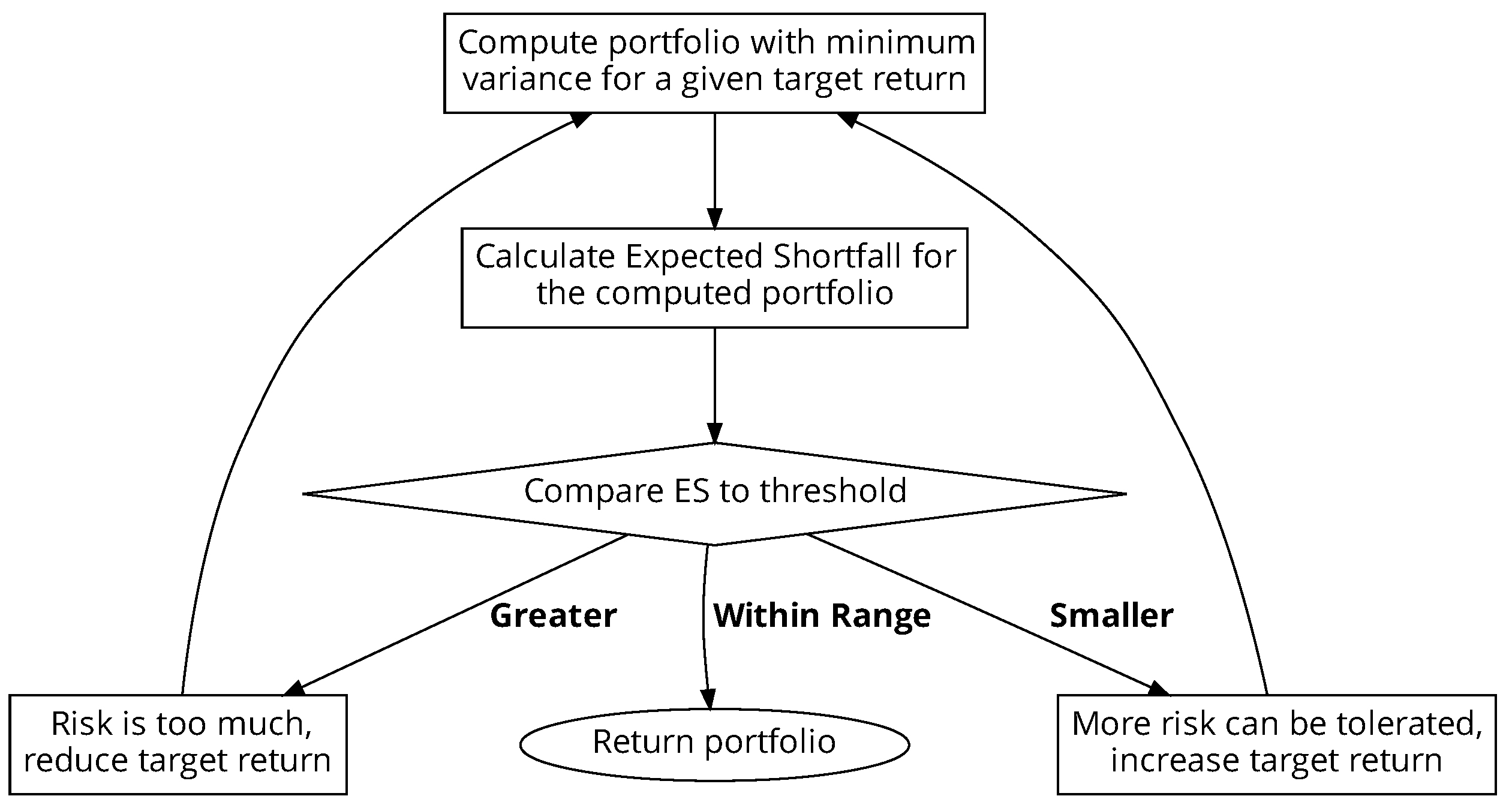
(P1) Minimize the expected shortfall under the constraints that the expected return is satisfied, the variance of the portfolio is small, and all assets are invested.
| Algorithm 1: Expected Shortfall based Dynamic Asset Allocation during t. |
 |
3. A Hybrid Quantum Classical Algorithm
3.1. Algorithm Overview
3.2. Previous Work
4. Experimental Setup and Results
4.1. D-Wave Quantum Annealer
4.2. Test Input and Annealer Parameters
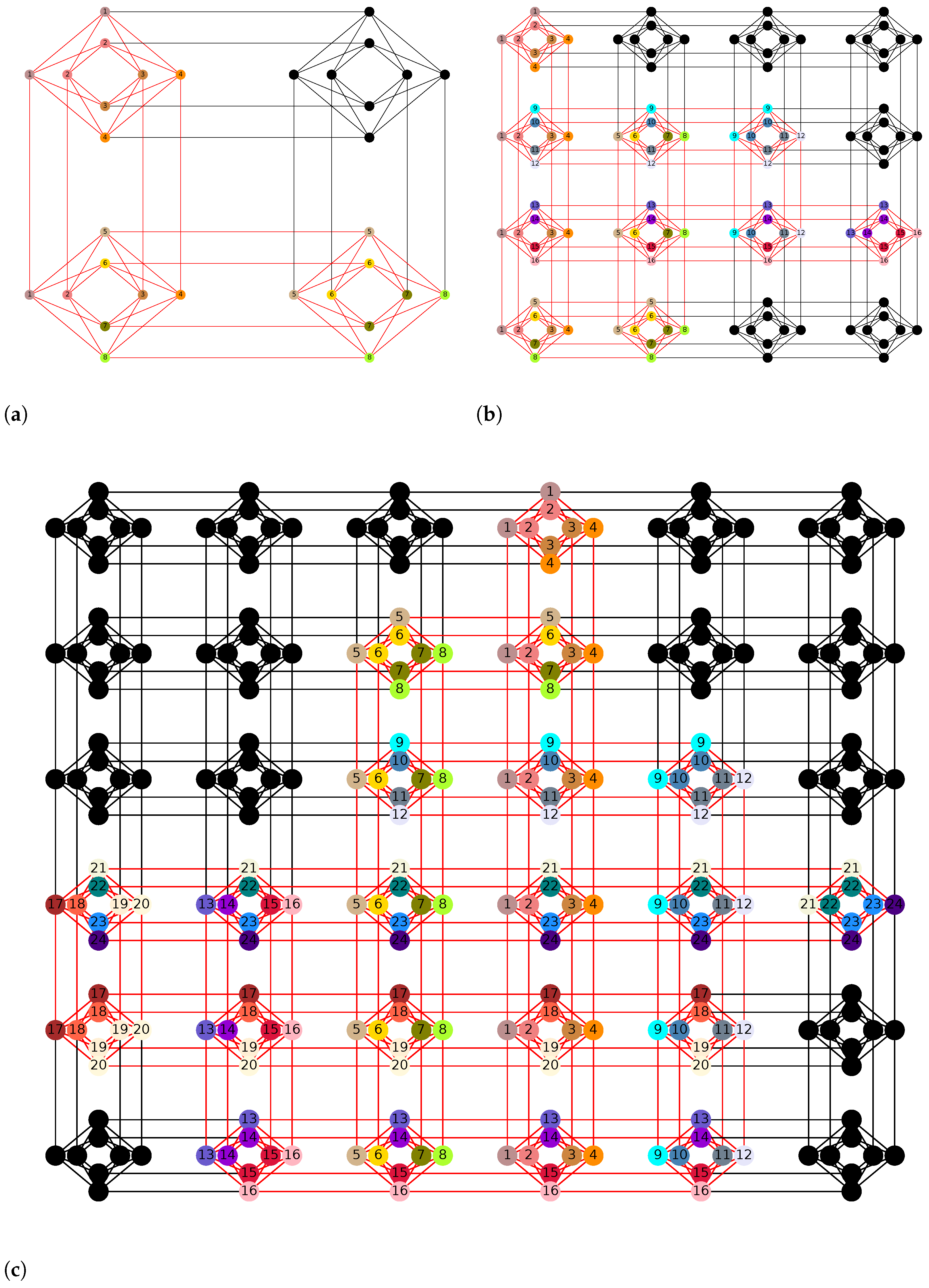
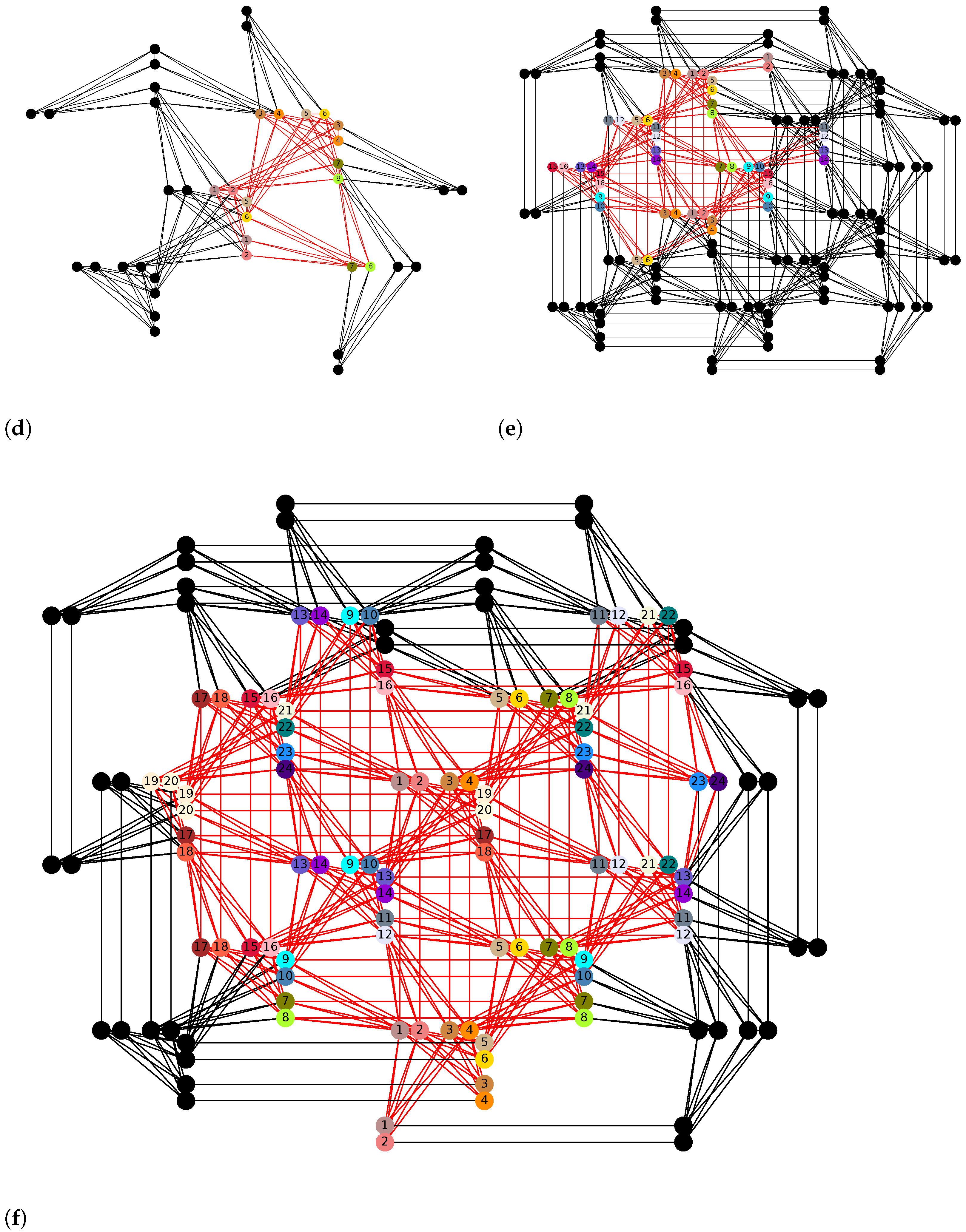
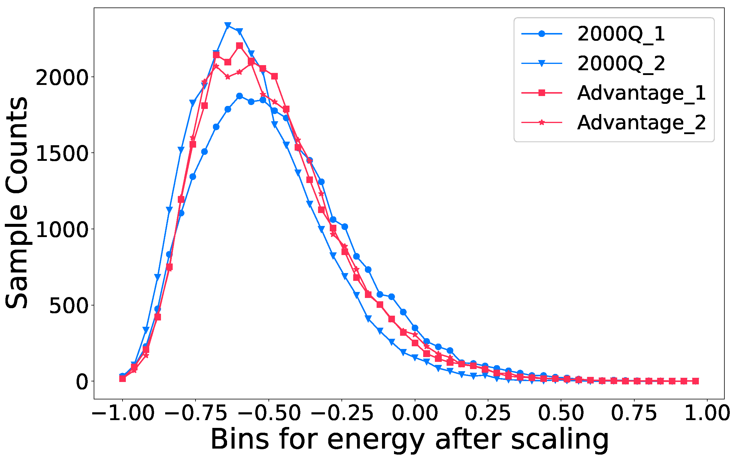
4.3. Embedding Comparison on D-Wave Annealers
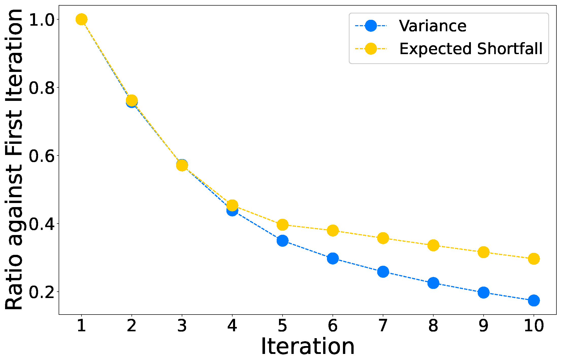
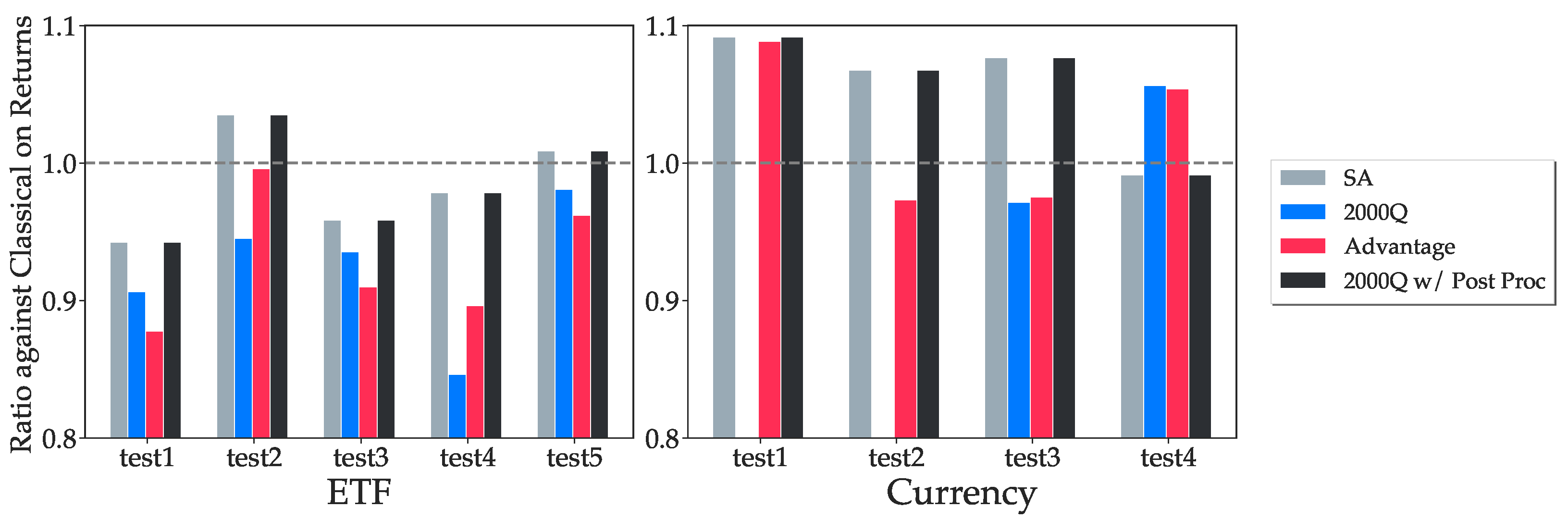
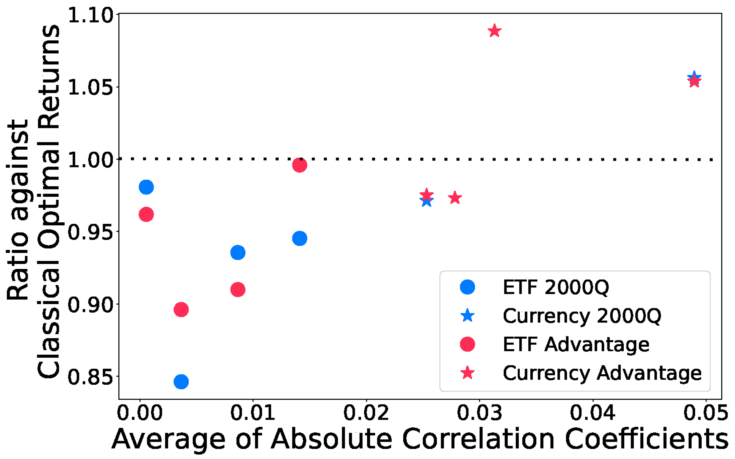
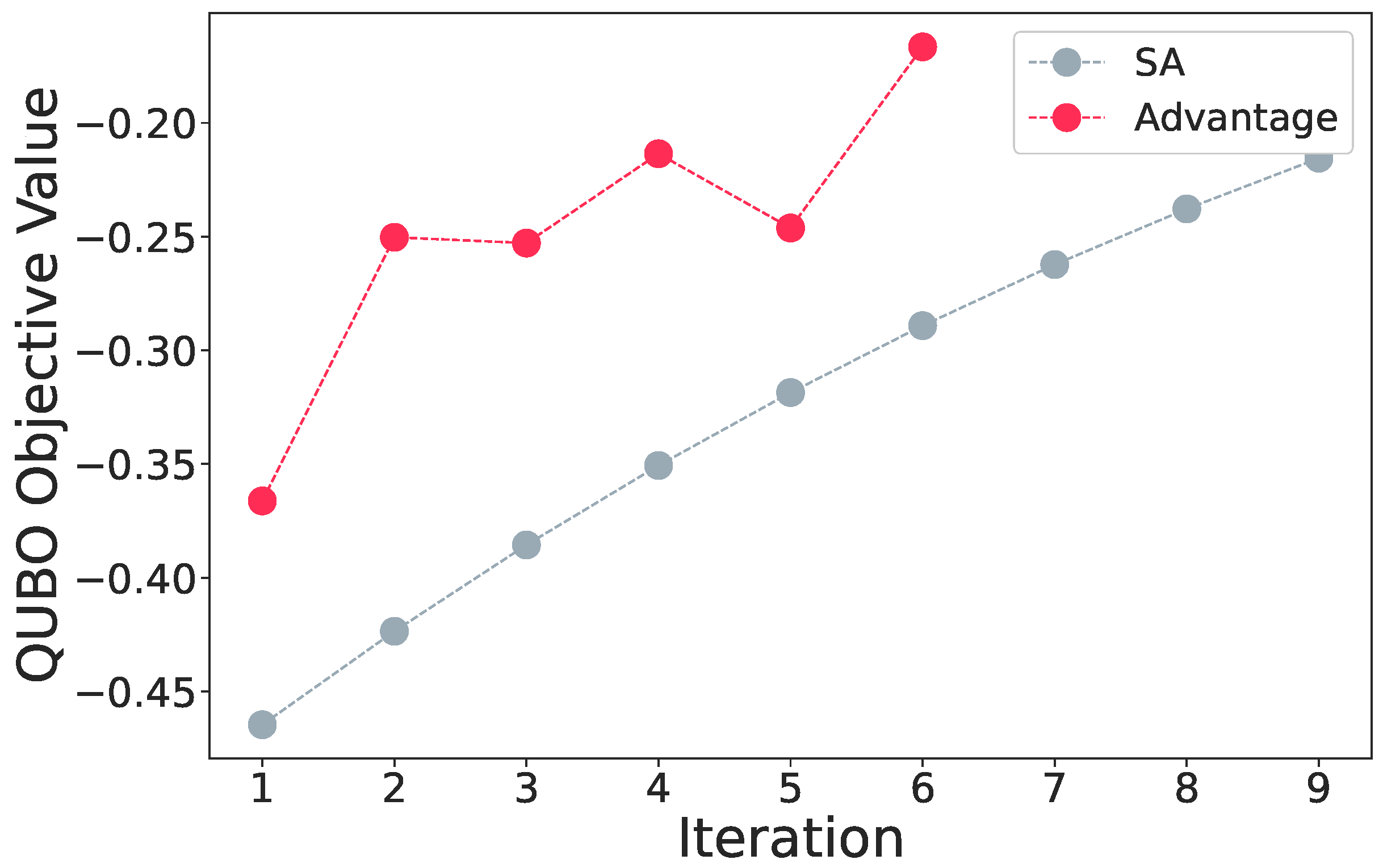
4.4. Annealing Results Comparison
4.5. State-of-the-Art on D-Wave Annealers
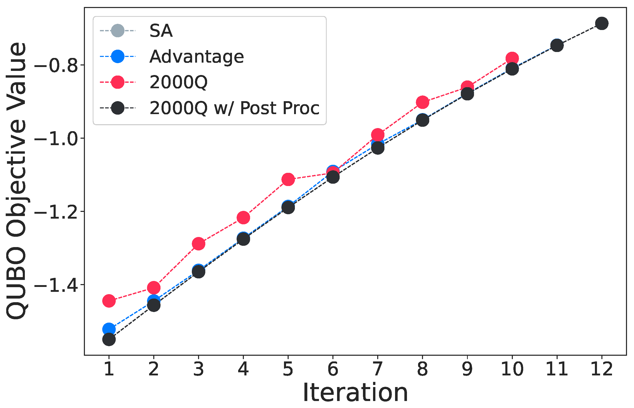
5. Discussion
Author Contributions
Funding
Institutional Review Board Statement
Data Availability Statement
Acknowledgments
Conflicts of Interest
References
- Glover, F.; Kochenberger, G.; Du, Y. A Tutorial on Formulating and Using QUBO Models. arXiv 2019, arXiv:1811.11538. [Google Scholar]
- Pastorello, D.; Blanzieri, E. Quantum Annealing Learning Search for Solving QUBO Problems. Quantum Inf. Process. 2019, 18, 303. [Google Scholar] [CrossRef] [Green Version]
- Kochenberger, G.; Hao, J.K.; Glover, F.; Lewis, M.; Lü, Z.; Wang, H.; Wang, Y. The Unconstrained Binary Quadratic Programming Problem: A Survey. J. Comb. Optim. 2014, 28, 58–81. [Google Scholar] [CrossRef] [Green Version]
- Lucas, A. Ising Formulations of Many NP Problems. Front. Phys. 2014, 2, 5. [Google Scholar] [CrossRef] [Green Version]
- Djidjev, H.N.; Chapuis, G.; Hahn, G.; Rizk, G. Efficient Combinatorial Optimization Using Quantum Annealing. arXiv 2018, arXiv:1801.08653. [Google Scholar]
- Ikeda, K.; Nakamura, Y.; Humble, T.S. Application of Quantum Annealing to Nurse Scheduling Problem. Sci. Rep. 2019, 9, 12837. [Google Scholar] [CrossRef] [PubMed] [Green Version]
- Titiloye, O.; Crispin, A. Quantum Annealing of the Graph Coloring Problem. Discret. Optim. 2011, 8, 376–384. [Google Scholar] [CrossRef] [Green Version]
- Yarkoni, S.; Raponi, E.; Bäck, T.; Schmitt, S. Quantum Annealing for Industry Applications: Introduction and Review. Rep. Prog. Phys. 2022, 85, 104001. [Google Scholar] [CrossRef]
- Markowitz, H. Portfolio Selection. J. Financ. 1952, 7, 77–91. [Google Scholar] [CrossRef]
- Black, F.; Litterman, R.B. Asset Allocation: Combining Investor Views with Market Equilibrium. J. Fixed Income 1991, 1, 7–18. [Google Scholar] [CrossRef]
- McNeil, A.J.; Frey, R.; Embrechts, P. Quantitative Risk Management: Concepts, Techniques and Tools—Revised Edition; Princeton University Press: Princeton, NJ, USA, 2015. [Google Scholar]
- Dasgupta, S.; Banerjee, A. Quantum Annealing Algorithm for Expected Shortfall Based Dynamic Asset Allocation. arXiv 2020, arXiv:1909.12904. [Google Scholar]
- Pardalos, P.M.; Vavasis, S.A. Quadratic Programming with One Negative Eigenvalue Is NP-hard. J. Glob. Optim. 1991, 1, 15–22. [Google Scholar] [CrossRef]
- Vavasis, S.A. Complexity Theory: Quadratic Programming. In Encyclopedia of Optimization; Floudas, C.A., Pardalos, P.M., Eds.; Springer: Boston, MA, USA, 2001; pp. 304–307. [Google Scholar] [CrossRef]
- Grant, E.; Humble, T.S.; Stump, B. Benchmarking Quantum Annealing Controls with Portfolio Optimization. Phys. Rev. Appl. 2021, 15, 014012. [Google Scholar] [CrossRef]
- O’Donnell, R. Analysis of Boolean Functions; Cambridge University Press: Cambridge, UK, 2014. [Google Scholar] [CrossRef]
- Dattani, N. Quadratization in Discrete Optimization and Quantum Mechanics. arXiv 2019, arXiv:1901.04405. [Google Scholar]
- Verma, A.; Lewis, M.; Kochenberger, G. Efficient QUBO Transformation for Higher Degree Pseudo Boolean Functions. arXiv 2021, arXiv:2107.11695. [Google Scholar]
- Mandal, A.; Roy, A.; Upadhyay, S.; Ushijima-Mwesigwa, H. Compressed Quadratization of Higher Order Binary Optimization Problems. In Proceedings of the 2020 Data Compression Conference (DCC), Snowbird, UT, USA, 24–27 March 2020; pp. 126–131. [Google Scholar] [CrossRef]
- Yahoo Finance iShares MSCI Emerging Markets ETF (EEM). Available online: https://finance.yahoo.com/quote/EEM/history?p=EEM (accessed on 18 May 2020).
- Yahoo Finance Invesco QQQ Trust (QQQ). Available online: https://finance.yahoo.com/quote/QQQ/history?p=QQQ (accessed on 18 May 2020).
- Yahoo Finance iShares Silver Trust (SLV). Available online: https://finance.yahoo.com/quote/SLV/history?p=SLV (accessed on 18 May 2020).
- Yahoo Finance SPDR S&P 500 ETF Trust (SPY). Available online: https://finance.yahoo.com/quote/SPY/history?p=SPY (accessed on 18 May 2020).
- Yahoo Finance ProShares UltraPro Short QQQ (SQQQ). Available online: https://finance.yahoo.com/quote/SQQQ/history?p=SQQQ (accessed on 18 May 2020).
- Yahoo Finance Financial Select Sector SPDR Fund (XLF). Available online: https://finance.yahoo.com/quote/XLF/history?p=XLF (accessed on 18 May 2020).
- Uryasev, S.; Rockafellar, R.T. Conditional Value-at-Risk: Optimization Approach. In Stochastic Optimization: Algorithms and Applications; Uryasev, S., Pardalos, P.M., Eds.; Applied Optimization; Springer: Boston, MA, USA, 2001; pp. 411–435. [Google Scholar] [CrossRef]
- Norton, M.; Khokhlov, V.; Uryasev, S. Calculating CVaR and bPOE for Common Probability Distributions with Application to Portfolio Optimization and Density Estimation. Ann. Oper. Res. 2021, 299, 1281–1315. [Google Scholar] [CrossRef] [Green Version]
- Bertsimas, D.; Lauprete, G.J.; Samarov, A. Shortfall as a Risk Measure: Properties, Optimization and Applications. J. Econ. Dyn. Control 2004, 28, 1353–1381. [Google Scholar] [CrossRef]
- Brooke, J.; Bitko, D.; Rosenbaum, T.F.; Aeppli, G. Quantum Annealing of a Disordered Magnet. Science 1999, 284, 779–781. [Google Scholar] [CrossRef] [Green Version]
- Santoro, G.E.; Martoňák, R.; Tosatti, E.; Car, R. Theory of Quantum Annealing of an Ising Spin Glass. Science 2002, 295, 2427–2430. [Google Scholar] [CrossRef] [Green Version]
- King, A.D.; Raymond, J.; Lanting, T.; Harris, R.; Zucca, A.; Altomare, F.; Berkley, A.J.; Boothby, K.; Ejtemaee, S.; Enderud, C.; et al. Quantum Critical Dynamics in a 5000-Qubit Programmable Spin Glass. arXiv 2022, arXiv:2207.13800. [Google Scholar]
- Venegas-Andraca, S.E.; Cruz-Santos, W.; McGeoch, C.; Lanzagorta, M. A Cross-Disciplinary Introduction to Quantum Annealing-Based Algorithms. Contemp. Phys. 2018, 59, 174–197. [Google Scholar] [CrossRef] [Green Version]
- Barahona, F. On the Computational Complexity of Ising Spin Glass Models. J. Phys. A Math. Gen. 1982, 15, 3241–3253. [Google Scholar] [CrossRef]
- Zhang, Z. Computational Complexity of Spin-Glass Three-Dimensional (3D) Ising Model. J. Mater. Sci. Technol. 2020, 44, 116–120. [Google Scholar] [CrossRef]
- Vinci, W.; Lidar, D.A. Non-Stoquastic Hamiltonians in Quantum Annealing via Geometric Phases. Npj Quantum Inf. 2017, 3, 1–6. [Google Scholar] [CrossRef] [Green Version]
- Farhi, E.; Goldstone, J.; Gutmann, S.; Sipser, M. Quantum Computation by Adiabatic Evolution. arXiv 2000, arXiv:quant-ph/0001106. [Google Scholar]
- Albash, T.; Lidar, D.A. Adiabatic Quantum Computation. Rev. Mod. Phys. 2018, 90, 015002. [Google Scholar] [CrossRef] [Green Version]
- Born, M.; Fock, V. Beweis des Adiabatensatzes. Z. für Phys. 1928, 51, 165–180. [Google Scholar] [CrossRef]
- D-Wave Systems Inc. The Practical Quantum Computing Company. ICE: Dynamic Ranges in h and J Values, 2021. [Google Scholar]
- Rosenberg, G.; Haghnegahdar, P.; Goddard, P.; Carr, P.; Wu, K.; de Prado, M.L. Solving the Optimal Trading Trajectory Problem Using a Quantum Annealer. IEEE J. Sel. Top. Signal Process. 2016, 10, 1053–1060. [Google Scholar] [CrossRef] [Green Version]
- Venturelli, D.; Kondratyev, A. Reverse Quantum Annealing Approach to Portfolio Optimization Problems. Quantum Mach. Intell. 2019, 1, 17–30. [Google Scholar] [CrossRef] [Green Version]
- Phillipson, F.; Bhatia, H.S. Portfolio Optimisation Using the D-Wave Quantum Annealer. In Proceedings of the Computational Science—ICCS 2021, Krakow, Poland, 16–18 June 2021; Lecture Notes in Computer Science. Paszynski, M., Kranzlmüller, D., Krzhizhanovskaya, V.V., Dongarra, J.J., Sloot, P.M.A., Eds.; Springer International Publishing: Cham, Switzerland, 2021; pp. 45–59. [Google Scholar] [CrossRef]
- Metropolis, N.; Rosenbluth, A.W.; Rosenbluth, M.N.; Teller, A.H.; Teller, E. Equation of State Calculations by Fast Computing Machines. J. Chem. Phys. 1953, 21, 1087–1092. [Google Scholar] [CrossRef] [Green Version]
- Kirkpatrick, S.; Gelatt, C.D.; Vecchi, M.P. Optimization by Simulated Annealing. Science 1983, 220, 671–680. [Google Scholar] [CrossRef]
- Liu, Y.J.; Zhang, W.G. A Multi-Period Fuzzy Portfolio Optimization Model with Minimum Transaction Lots. Eur. J. Oper. Res. 2015, 242, 933–941. [Google Scholar] [CrossRef]
- Vercher, E.; Bermúdez, J.D. Portfolio Optimization Using a Credibility Mean-Absolute Semi-Deviation Model. Expert Syst. Appl. 2015, 42, 7121–7131. [Google Scholar] [CrossRef]
- Mansini, R.; Ogryczak, W.; Speranza, M.G. Twenty Years of Linear Programming Based Portfolio Optimization. Eur. J. Oper. Res. 2014, 234, 518–535. [Google Scholar] [CrossRef]
- Schaerf, A. Local Search Techniques for Constrained Portfolio Selection Problems. Comput. Econ. 2002, 20, 177–190. [Google Scholar] [CrossRef]
- Hegade, N.N.; Chandarana, P.; Paul, K.; Chen, X.; Albarrán-Arriagada, F.; Solano, E. Portfolio Optimization with Digitized-Counterdiabatic Quantum Algorithms. Phys. Rev. Res. 2022, 4, 043204. [Google Scholar] [CrossRef]
- D-Wave Systems Inc. The Practical Quantum Computing Company. The D-Wave Advantage System: An Overview. 2021. Available online: https://www.dwavesys.com/media/s3qbjp3s/14-1049a-a_the_d-wave_advantage_system_an_overview.pdf (accessed on 18 May 2020).
- Venturelli, D.; Mandrà, S.; Knysh, S.; O’Gorman, B.; Biswas, R.; Smelyanskiy, V. Quantum Optimization of Fully Connected Spin Glasses. Phys. Rev. X 2015, 5, 031040. [Google Scholar] [CrossRef] [Green Version]
- Boothby, T.; King, A.D.; Roy, A. Fast Clique Minor Generation in Chimera Qubit Connectivity Graphs. Quantum Inf. Process. 2016, 15, 495–508. [Google Scholar] [CrossRef] [Green Version]
- Pelofske, E.; Hahn, G.; Djidjev, H. Optimizing the Spin Reversal Transform on the D-Wave 2000Q. In Proceedings of the 2019 IEEE International Conference on Rebooting Computing (ICRC), San Mateo, CA, USA, 6–8 November 2019; pp. 1–8. [Google Scholar] [CrossRef] [Green Version]
- Lanting, T.; Amin, M.H.; Baron, C.; Babcock, M.; Boschee, J.; Boixo, S.; Smelyanskiy, V.N.; Foygel, M.; Petukhov, A.G. Probing Environmental Spin Polarization with Superconducting Flux Qubits. arXiv 2020, arXiv:2003.14244. [Google Scholar]
- Pudenz, K.L. Parameter Setting for Quantum Annealers. In Proceedings of the 2016 IEEE High Performance Extreme Computing Conference (HPEC), Waltham, MA, USA, 13–15 September 2016; pp. 1–6. [Google Scholar] [CrossRef] [Green Version]
- Markowitz, H.M. The Elimination Form of the Inverse and Its Application to Linear Programming. Manag. Sci. 1957, 3, 255–269. [Google Scholar] [CrossRef]
- Jensen, F.V.; Lauritzen, S.L.; Olesen, K.G. Bayesian Updating in Causal Probabilistic Networks by Local Computations. Comput. Stat. Q. 1990, 4, 269–282. [Google Scholar]
- Diamond, S.; Boyd, S.P. CVXPY: A Python-Embedded Modeling Language for Convex Optimization. J. Mach. Learn. Res. 2016, 17, 2909–2913. [Google Scholar]
- Barbosa, A.; Pelofske, E.; Hahn, G.; Djidjev, H.N. Using Machine Learning for Quantum Annealing Accuracy Prediction. Algorithms 2021, 14, 187. [Google Scholar] [CrossRef]
- Farhi, E.; Goldstone, J.; Gutmann, S. A Quantum Approximate Optimization Algorithm. arXiv 2014, arXiv:1411.4028. [Google Scholar]
- Hadfield, S.; Wang, Z.; O’Gorman, B.; Rieffel, E.G.; Venturelli, D.; Biswas, R. From the Quantum Approximate Optimization Algorithm to a Quantum Alternating Operator Ansatz. Algorithms 2019, 12, 34. [Google Scholar] [CrossRef] [Green Version]


| Embedding | Average Objective | Best Objective |
|---|---|---|
| 1 | ||
| 2 | ||
| 3 | ||
| 4 |
| Embedding | Average Objective | Best Objective |
|---|---|---|
| 1 | 99.25% | 99.89% |
| 2 | 99.52% | 99.94% |
| 3 | 99.22% | 99.95% |
| 4 | 99.48% | 99.89% |
| Last k Iteration | SA Objective | Advantage Objective | Difference |
|---|---|---|---|
| 5 | −1.026 | −1.016 | 1.039% |
| 4 | −0.951 | −0.950 | 0.092% |
| 3 | −0.879 | −0.878 | 0.111% |
| 2 | −0.811 | −0.809 | 0.170% |
| 1 | −0.746 | −0.746 | 0.076% |
Disclaimer/Publisher’s Note: The statements, opinions and data contained in all publications are solely those of the individual author(s) and contributor(s) and not of MDPI and/or the editor(s). MDPI and/or the editor(s) disclaim responsibility for any injury to people or property resulting from any ideas, methods, instructions or products referred to in the content. |
© 2023 by the authors. Licensee MDPI, Basel, Switzerland. This article is an open access article distributed under the terms and conditions of the Creative Commons Attribution (CC BY) license (https://creativecommons.org/licenses/by/4.0/).
Share and Cite
Xu, H.; Dasgupta, S.; Pothen, A.; Banerjee, A. Dynamic Asset Allocation with Expected Shortfall via Quantum Annealing. Entropy 2023, 25, 541. https://doi.org/10.3390/e25030541
Xu H, Dasgupta S, Pothen A, Banerjee A. Dynamic Asset Allocation with Expected Shortfall via Quantum Annealing. Entropy. 2023; 25(3):541. https://doi.org/10.3390/e25030541
Chicago/Turabian StyleXu, Hanjing, Samudra Dasgupta, Alex Pothen, and Arnab Banerjee. 2023. "Dynamic Asset Allocation with Expected Shortfall via Quantum Annealing" Entropy 25, no. 3: 541. https://doi.org/10.3390/e25030541