
Dynamics of Quantum Networks in Noisy Environments

Abstract
:1. Introduction
2. Preliminaries
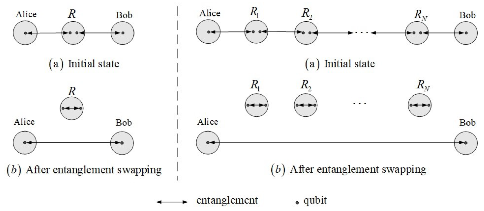
2.1. Quantum Network Model
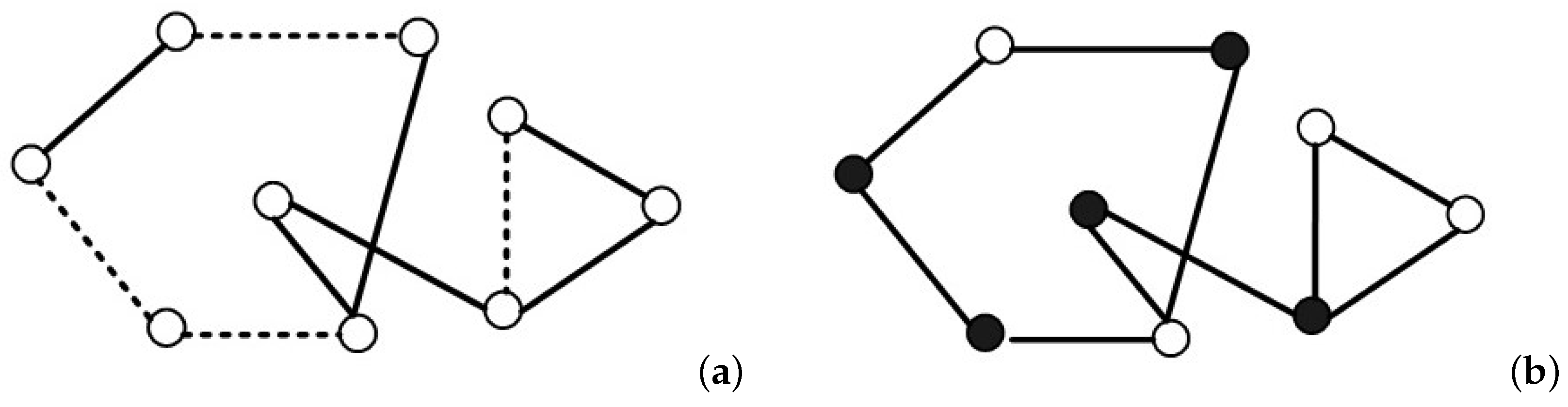
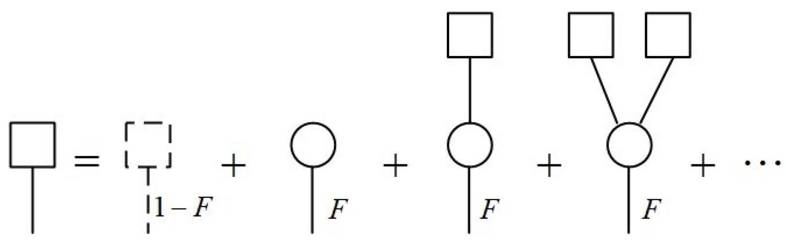
2.2. Percolation Model
3. The Evolution of Quantum Network
3.1. Analytical Framework
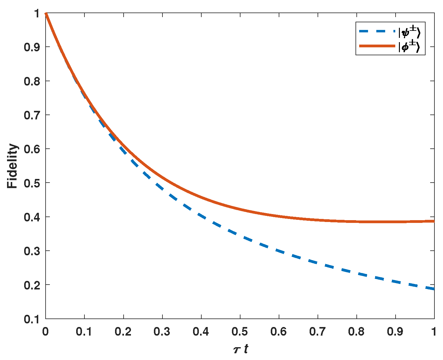
3.2. Amplitude Damping and Phase Damping Noises
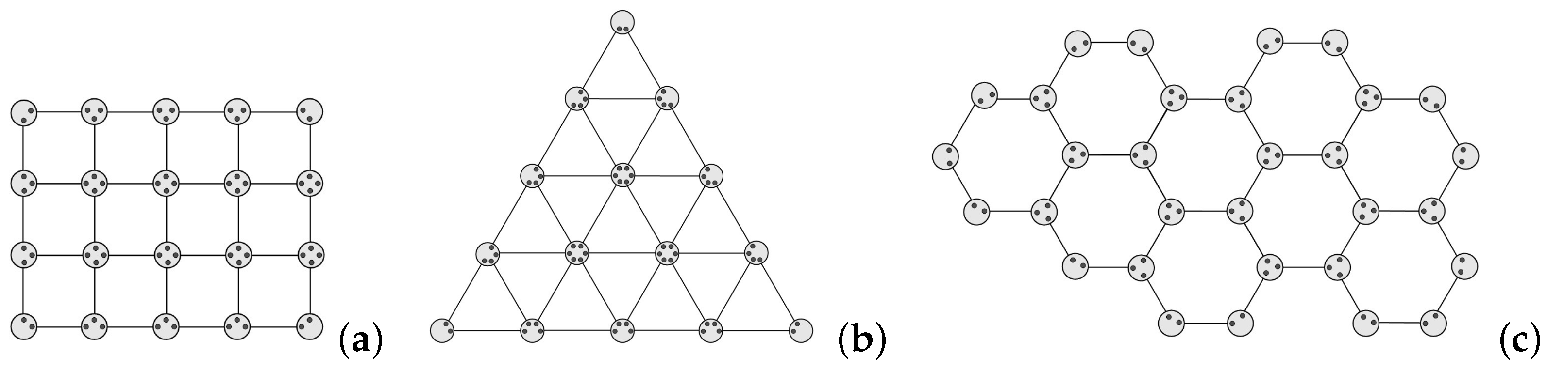
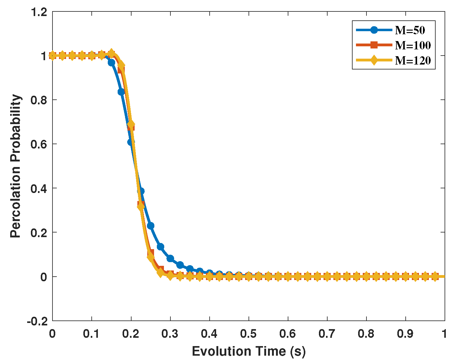
3.3. Regular Quantum Networks
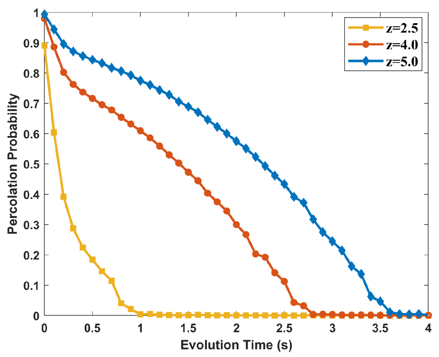
3.4. Complex Quantum Networks
4. The Capacity of Quantum Networks
5. Conclusions
Author Contributions
Funding
Institutional Review Board Statement
Data Availability Statement
Conflicts of Interest
Abbreviations
| QKD | Quantum Key Distribution |
| GCC | Giant Connected Component |
| FCC | Finite Connected Component |
| NMR | Nuclear Magnetic Resonance |
References
- Bennett, C.H.; Brassard, G. Quantum Cryptography: Public Key Distribution and Coin Tossing. In Proceedings of the IEEE International Conference on Computers. Systems and Signal Processing, Bangalore, India, 10–12 December 1984. [Google Scholar]
- Tomita, A. Implementation security certification of decoy-BB84 quantum key distribution systems. Adv. Quantum Technol. 2019, 2, 1900005. [Google Scholar] [CrossRef]
- Wang, X.B.; Yu, Z.W.; Hu, X.L. Twin-field quantum key distribution with large misalignment error. Phys. Rev. A 2018, 98, 062323. [Google Scholar] [CrossRef] [Green Version]
- Ma, X.F.; Zeng, P.; Zhou, H.Y. Phase-matching quantum key distribution. Phys. Rev. X 2018, 8, 031043. [Google Scholar] [CrossRef] [Green Version]
- Elliott1, C.; Colvin, A.; Pearson, D.; Pikalo, O.; Schlafer, J.; Yeh, H. Current status of the DARPA quantum network. Proc. SPIE Int. Soc. Opt. Eng. 2005, 5815, 138–149. [Google Scholar]
- Sasaki, M.; Fujiwara, M.; Ishizuka, H.; Klaus, W.; Wakui, K.; Takeoka, M.; Miki, S.; Yamashita, T.; Wang, Z.; Tanaka, A.; et al. Field test of quantum key distribution in the Tokyo QKD Network. Opt. Express 2011, 19, 10387–10409. [Google Scholar] [CrossRef] [PubMed]
- Liao, S.K.; Cai, W.Q.; Handsteiner, J.; Liu, B.; Yin, J.; Zhang, L.; Rauch, D.; Fink, M.; Ren, J.G.; Liu, W.Y.; et al. Satellite-relayed intercontinental quantum network. Phys. Rev. Lett. 2018, 120, 030501. [Google Scholar] [CrossRef] [PubMed] [Green Version]
- Nielsen, M.A.; Chuang, I.L. Quantum Computation and Quantum Information; Cambridge University Press: Cambridge, UK, 2000. [Google Scholar]
- Gyongyosi, L. Dynamics of entangled networks of the quantum Internet. Sci. Rep. 2020, 10, 12909. [Google Scholar] [CrossRef] [PubMed]
- Santra, S.; Malinovsky, V.S. Quantum networking with short-range entanglement assistance. Phys. Rev. A 2021, 103, 012407. [Google Scholar] [CrossRef]
- Bennett, C.H.; Brassard, G.; Crépeau, C.; Jozsa, R.; Peres, A.; Wootters, W.K. Teleporting an unknown quantum state via dual classical and Einstein-Podolsky-Rosen channels. Phys. Rev. Lett. 1993, 70, 1895–1899. [Google Scholar] [CrossRef] [Green Version]
- Acín, A.; Cirac, J.I.; Lewenstein, M. Entanglement percolation in quantum network. Nat. Phys. 2007, 3, 256–259. [Google Scholar] [CrossRef] [Green Version]
- Grimmett, G.R. Percolation; Springer: Berlin/Heidelberg, Germany, 1999. [Google Scholar]
- Cuquet, M.; Calsamiglia, J. Entanglement percolation in quantum complex networks. Phys. Rev. Lett. 2009, 103, 240503. [Google Scholar] [CrossRef]
- Perseguers, S.; Cavalcanti, D.; Lapeyre, G.J., Jr.; Lewenstein, M.; Acín, A. Multipartite entanglement percolation. Phys. Rev. A 2010, 81, 032327. [Google Scholar] [CrossRef] [Green Version]
- Cuquet, M.; Calsamiglia, J. Limited-path-length entanglement percolation in quantum complex networks. Phys. Rev. A 2011, 83, 032319. [Google Scholar] [CrossRef] [Green Version]
- Wu, A.K.; Tian, L.; Coutinho, B.C.; Omar, Y.; Liu, Y.Y. Structural vulnerability of quantum networks. Phys. Rev. A 2020, 101, 052315. [Google Scholar] [CrossRef]
- Bennett, C.H.; Brassard, G.; Popescu, S.; Schumacher, B.; Smolin, J.A.; Wootters, W.K. Purification of noisy entanglement and faithful teleportation via noisy channel. Phys. Rev. Lett. 1996, 76, 722–725. [Google Scholar] [CrossRef] [PubMed] [Green Version]
- Fortes, R.; Rigolin, G. Fighting noise with noise in realistic quantum teleportation. Phys. Rev. A 2015, 92, 012338. [Google Scholar] [CrossRef] [Green Version]
- Knoll, L.T.; Schmiegelow, C.T.; Larotonda, M.A. Noisy quantum teleportation: An experimental study on the influence of local environments. Phys. Rev. A 2014, 90, 042332. [Google Scholar] [CrossRef] [Green Version]
- Jung, E.; Hwang, M.R.; Ju, Y.H.; Kim, M.S.; Yoo, S.K.; Kim, H.; Park, D.; Son, J.W.; Tamaryan, S.; Cha, S.K. Greenberger-Horne-Zeilinger versus W states: Quantum teleportation through noisy channels. Phys. Rev. A 2008, 78, 012312. [Google Scholar] [CrossRef] [Green Version]
- Oh, S.; Lee, S.; Lee, H.W. Fidelity of quantum teleportation through noisy channels. Phys. Rev. A 2002, 66, 022316. [Google Scholar] [CrossRef] [Green Version]
- Li, X.H.; Deng, F.G.; Zhou, H.Y. Efficient quantum key distribution over a collective noise channel. Phys. Rev. A 2008, 78, 022321. [Google Scholar] [CrossRef] [Green Version]
- Zhang, C.Y.; Zheng, Z.J. Entanglement-based quantum key distribution with untrusted third party. Quantum Inf. Process. 2021, 20, 146. [Google Scholar] [CrossRef]
- Huang, D.; Huang, P.; Lin, D.; Zeng, G. Long-distance continuous-variable quantum key distribution by controlling excess noise. Sci. Rep. 2016, 6, 19201. [Google Scholar] [CrossRef] [PubMed] [Green Version]
- Qu, Z.; Wu, S.; Wang, M.; Sun, L.; Wang, X. Effect of quantum noise on deterministic remote state preparation of an arbitrary two-particle state via various quantum entangled channels. Quantum Inf. Process. 2017, 16, 306. [Google Scholar] [CrossRef]
- Zhang, C.Y.; Bai, M.Q.; Zhou, S.Q. Cyclic joint remote state preparation in noisy environment. Quantum Inf. Process. 2018, 17, 146. [Google Scholar] [CrossRef]
- Passian, A.; Imam, N. Nanosystems, Edge Computing, and the Next Generation Computing Systems. Sensors 2019, 19, 4048. [Google Scholar] [CrossRef] [Green Version]
- Zukowski, M.; Zeilinger, A.; Horne, M.A.; Ekert, A.K. ‘Event-ready-detectors’ Bell experiment via entanglement swapping. Phys. Rev. Lett. 1993, 71, 4287–4290. [Google Scholar] [CrossRef]
- Yuan, Z.S.; Chen, Y.A.; Zhao, B.; Chen, S.; Schmiedmayer, J.; Pan, J.W. Experimental demonstration of a BDCZ quantum repeater node. Nature 2008, 454, 1098. [Google Scholar] [CrossRef] [Green Version]
- Bernien, H.; Hensen, B.; Pfaff, W.; Koolstra, G.; Blok, M.S.; Robledo, L.; Taminiau, T.H.; Markham, M.; Twitchen, D.J.; Childress, L.; et al. Heralded entanglement between solid-state qubits separated by three metres. Nature 2013, 497, 86–90. [Google Scholar] [CrossRef] [Green Version]
- Moehring, D.L.; Maunz, P.; Olmschenk, S.; Younge, K.C.; Matsukevich, D.N.; Duan, L.M.; Monroe, C. Entanglement of single-atom quantum bits at a distance. Nature 2007, 449, 68–71. [Google Scholar] [CrossRef] [Green Version]
- Stauffer, D.; Aharony, A. Introduction To Percolation Theory; Taylor & Francis: London, UK, 2018. [Google Scholar]
- Chayes, L.; Schonmann, R.H. Mixed Percolation as a bridge between site and bond percoaltion. Ann. Appl. Probab. 2000, 10, 1182. [Google Scholar] [CrossRef]
- Yanuka, M. The Mixed Bond-Site Percolation Problem and Its Application to Capillary Phenomena in Porous Media. J. Colloid Interface Sci. 1990, 134, 198. [Google Scholar] [CrossRef]
- González-Flores, M.I.; Torres, A.A.; Lebrecht, W.; Ramirez-Pastor, A.J. Site-bond percolation in two-dimensional kagome lattices: Analytical approach and numerical simulations. Phys. Rev. E 2021, 104, 014130. [Google Scholar] [CrossRef] [PubMed]
- Lindblad, G. On the generators of quantum dynamical semigroups. Commun. Math. Phys. 1976, 48, 119–130. [Google Scholar] [CrossRef]
- Uhlmann, A. The ‘transition probabilit’ in the state space of a ∗-algebra. Rep. Math. Phys. 1976, 9, 273–279. [Google Scholar] [CrossRef]
- Harpreet Singh, A.; Dorai, K. Using a Lindbladian approach to model decoherence in two coupled nuclear spins via correlated phase damping and amplitude damping noise channels. Pramana J. Phys. 2020, 94, 160. [Google Scholar] [CrossRef]
- Gupta, P.; Kumar, P.R. The capacity of wireless networks. IEEE Trans. Inf. Theory 2000, 46, 388. [Google Scholar] [CrossRef] [Green Version]
- Zhou, X.Z.; Yu, X.T. Capacity of a continuously distributed quantum network. Phys. Rev. A 2018, 98, 012316. [Google Scholar] [CrossRef]


| Lattice | Bond Percolation |
|---|---|
| 1d-Chain | 1 |
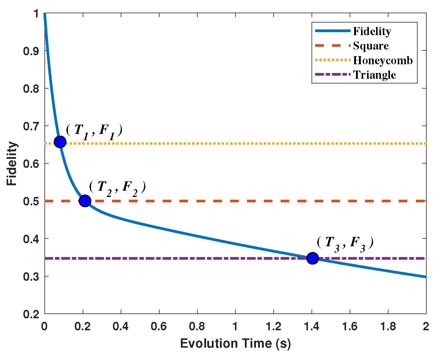
| 2d-Honeycomb | 1 − 2sin(/18) ≈ 0.6527 |
| 2d-Square | 0.5 |
| 2d-Triangle | 2sin(/18) ≈ 0.3473 |
Disclaimer/Publisher’s Note: The statements, opinions and data contained in all publications are solely those of the individual author(s) and contributor(s) and not of MDPI and/or the editor(s). MDPI and/or the editor(s) disclaim responsibility for any injury to people or property resulting from any ideas, methods, instructions or products referred to in the content. |
© 2023 by the authors. Licensee MDPI, Basel, Switzerland. This article is an open access article distributed under the terms and conditions of the Creative Commons Attribution (CC BY) license (https://creativecommons.org/licenses/by/4.0/).
Share and Cite
Zhang, C.-Y.; Zheng, Z.-J.; Fei, S.-M.; Feng, M. Dynamics of Quantum Networks in Noisy Environments. Entropy 2023, 25, 157. https://doi.org/10.3390/e25010157
Zhang C-Y, Zheng Z-J, Fei S-M, Feng M. Dynamics of Quantum Networks in Noisy Environments. Entropy. 2023; 25(1):157. https://doi.org/10.3390/e25010157
Chicago/Turabian StyleZhang, Chang-Yue, Zhu-Jun Zheng, Shao-Ming Fei, and Mang Feng. 2023. "Dynamics of Quantum Networks in Noisy Environments" Entropy 25, no. 1: 157. https://doi.org/10.3390/e25010157