Figure 1.
The von Neumann entropy of a matrix generated with a uniform eigenvalue distribution with no noise (left), Gaussian noise with standard deviation = 0.1 (middle), and Gaussian noise with standard deviation = 1 (right).
Figure 1.
The von Neumann entropy of a matrix generated with a uniform eigenvalue distribution with no noise (left), Gaussian noise with standard deviation = 0.1 (middle), and Gaussian noise with standard deviation = 1 (right).
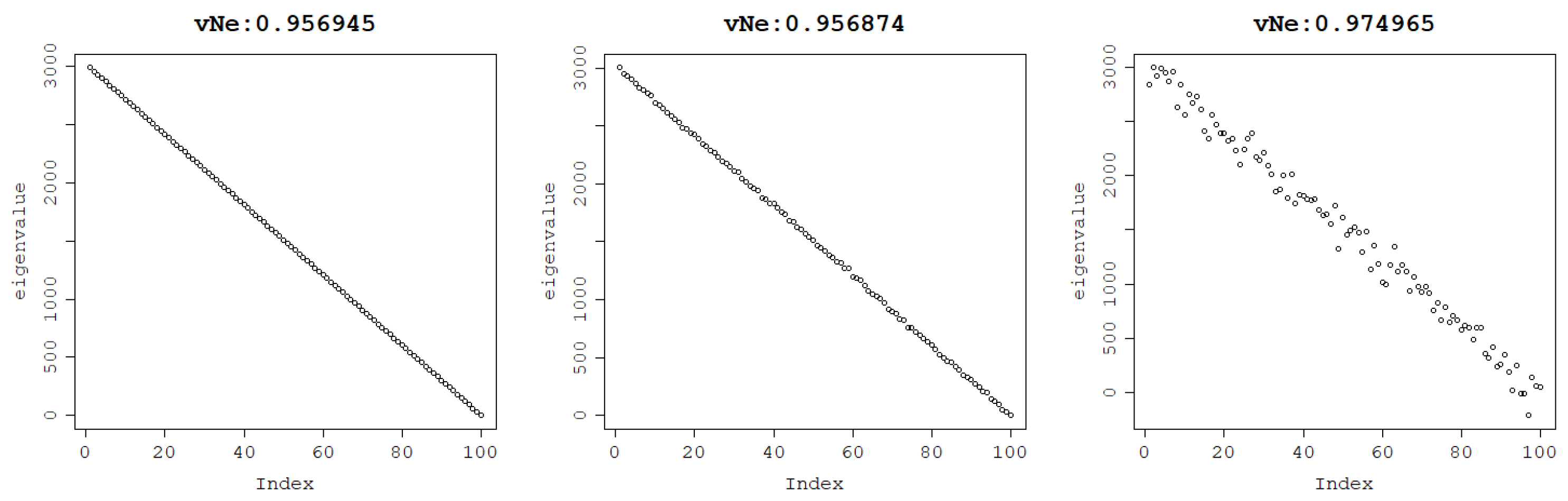
Figure 2.
The von Neumann entropy of a matrix generated with eigenvalues decreasing linearly with no noise (left), Gaussian noise with standard deviation = 10 (middle), and Gaussian noise with standard deviation = 100 (right).
Figure 2.
The von Neumann entropy of a matrix generated with eigenvalues decreasing linearly with no noise (left), Gaussian noise with standard deviation = 10 (middle), and Gaussian noise with standard deviation = 100 (right).
Figure 3.
The von Neumann entropy of a matrix generated with eigenvalues decreasing along a hyperbole with varying offset ranging from a = 0, a = 0.1, a = 1 to a = 10, respectively from left to right.
Figure 3.
The von Neumann entropy of a matrix generated with eigenvalues decreasing along a hyperbole with varying offset ranging from a = 0, a = 0.1, a = 1 to a = 10, respectively from left to right.
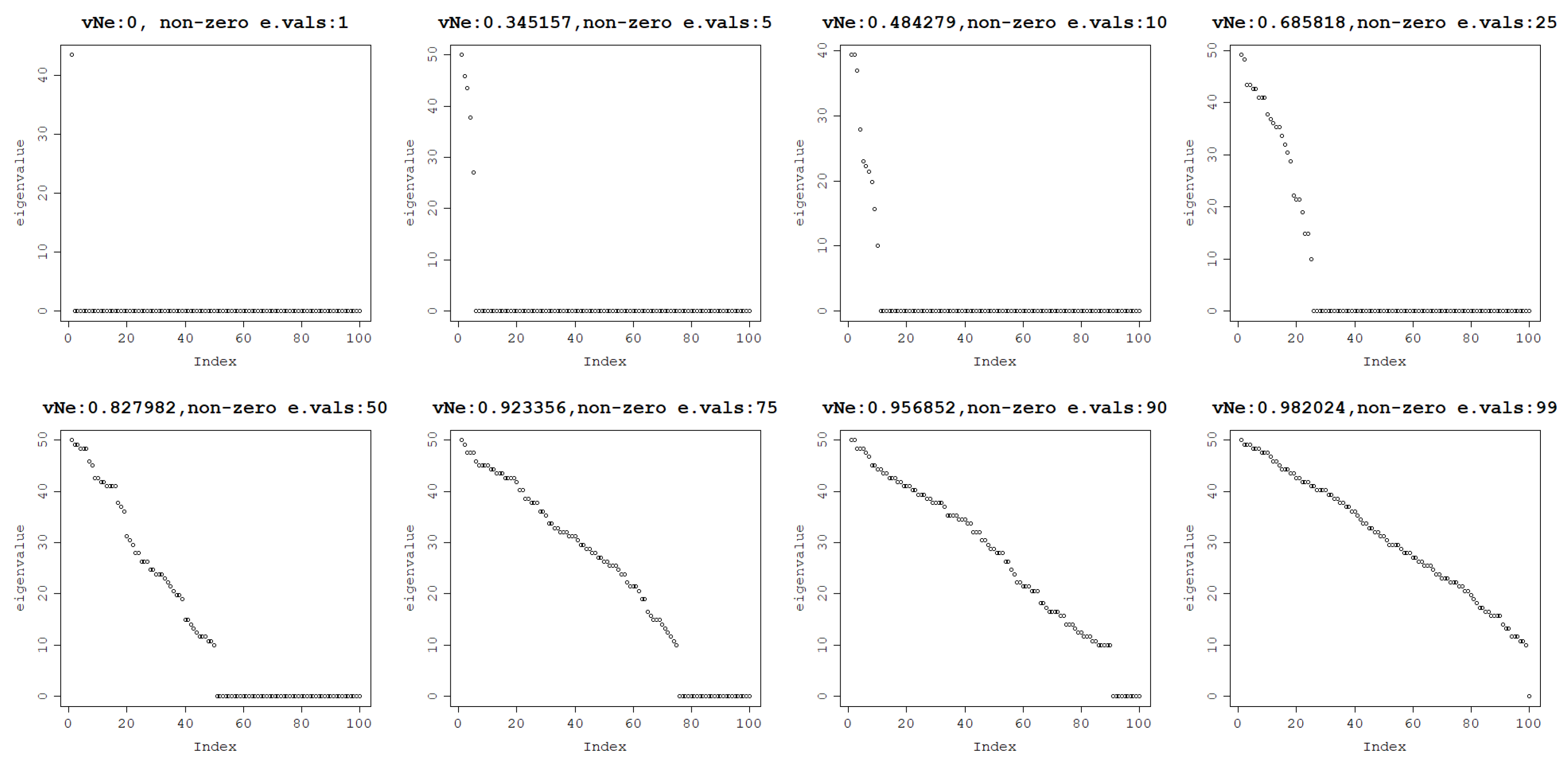
Figure 4.
The von Neumann entropy of a matrix generated with a varying number of non-zero eigenvalues: 1, 5, 10, 25, 50, 75, 90, 99, respectively, from the top left to the bottom right.
Figure 4.
The von Neumann entropy of a matrix generated with a varying number of non-zero eigenvalues: 1, 5, 10, 25, 50, 75, 90, 99, respectively, from the top left to the bottom right.
Figure 5.
Effect of normalizing the kernel matrix and scaling data rows to unit length on the von Neumann entropy, depending on the degree of the normalized polynomial kernel per dataset.
Figure 5.
Effect of normalizing the kernel matrix and scaling data rows to unit length on the von Neumann entropy, depending on the degree of the normalized polynomial kernel per dataset.
Figure 6.
Effect of scaling data rows to unit length on the von Neumann entropy depending on the kernel width of the RBF kernel per dataset.
Figure 6.
Effect of scaling data rows to unit length on the von Neumann entropy depending on the kernel width of the RBF kernel per dataset.
Figure 7.
Modeling the relationship between the RBF kernel width and the von Neumann entropy (in black) using a logarithm of a chosen base (in red) per dataset.
Figure 7.
Modeling the relationship between the RBF kernel width and the von Neumann entropy (in black) using a logarithm of a chosen base (in red) per dataset.
Figure 8.
Modeling the relationship between a normalized polynomial kernel degree and the von Neumann entropy (in black) using a logarithm of a chosen base (in red) per dataset.
Figure 8.
Modeling the relationship between a normalized polynomial kernel degree and the von Neumann entropy (in black) using a logarithm of a chosen base (in red) per dataset.
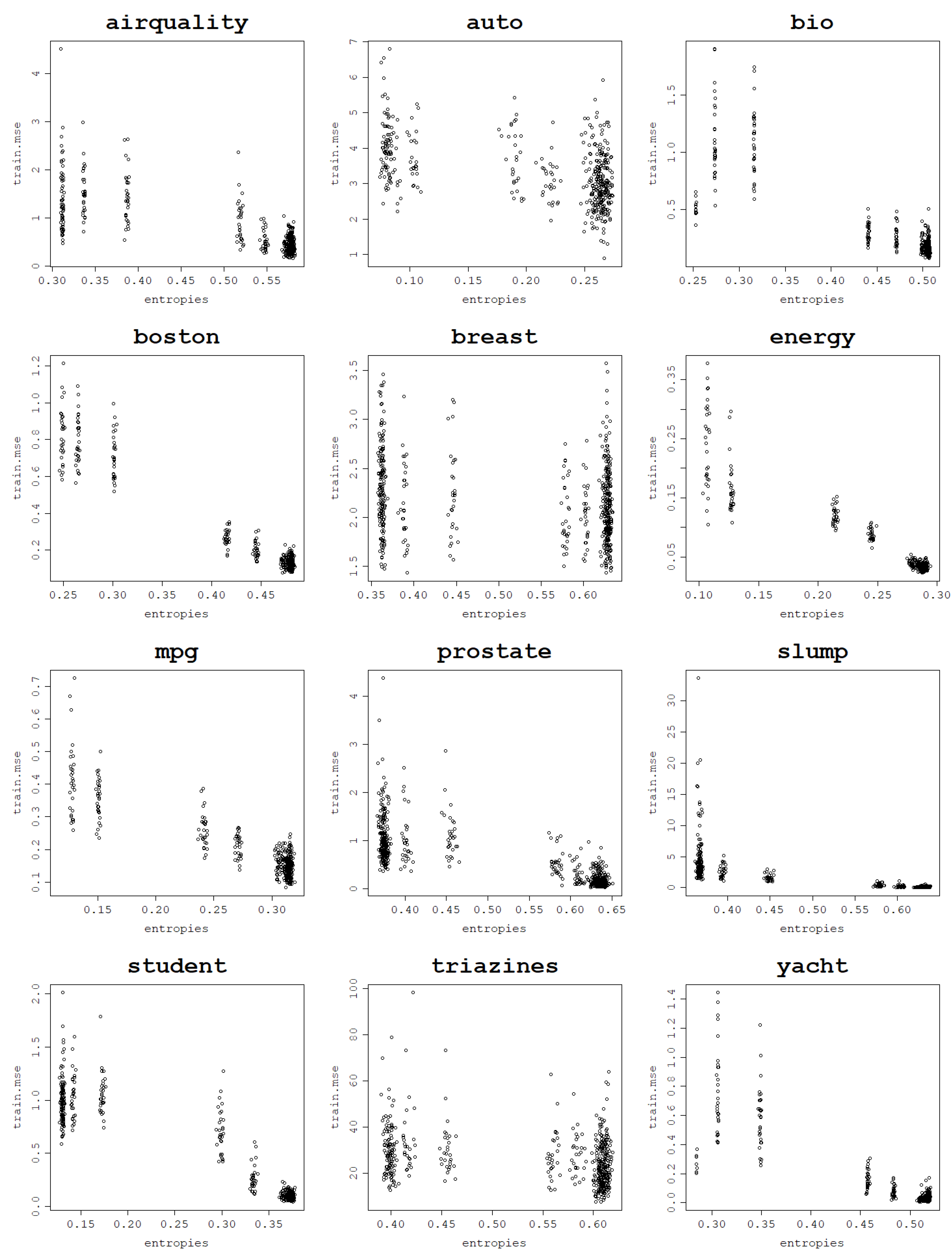
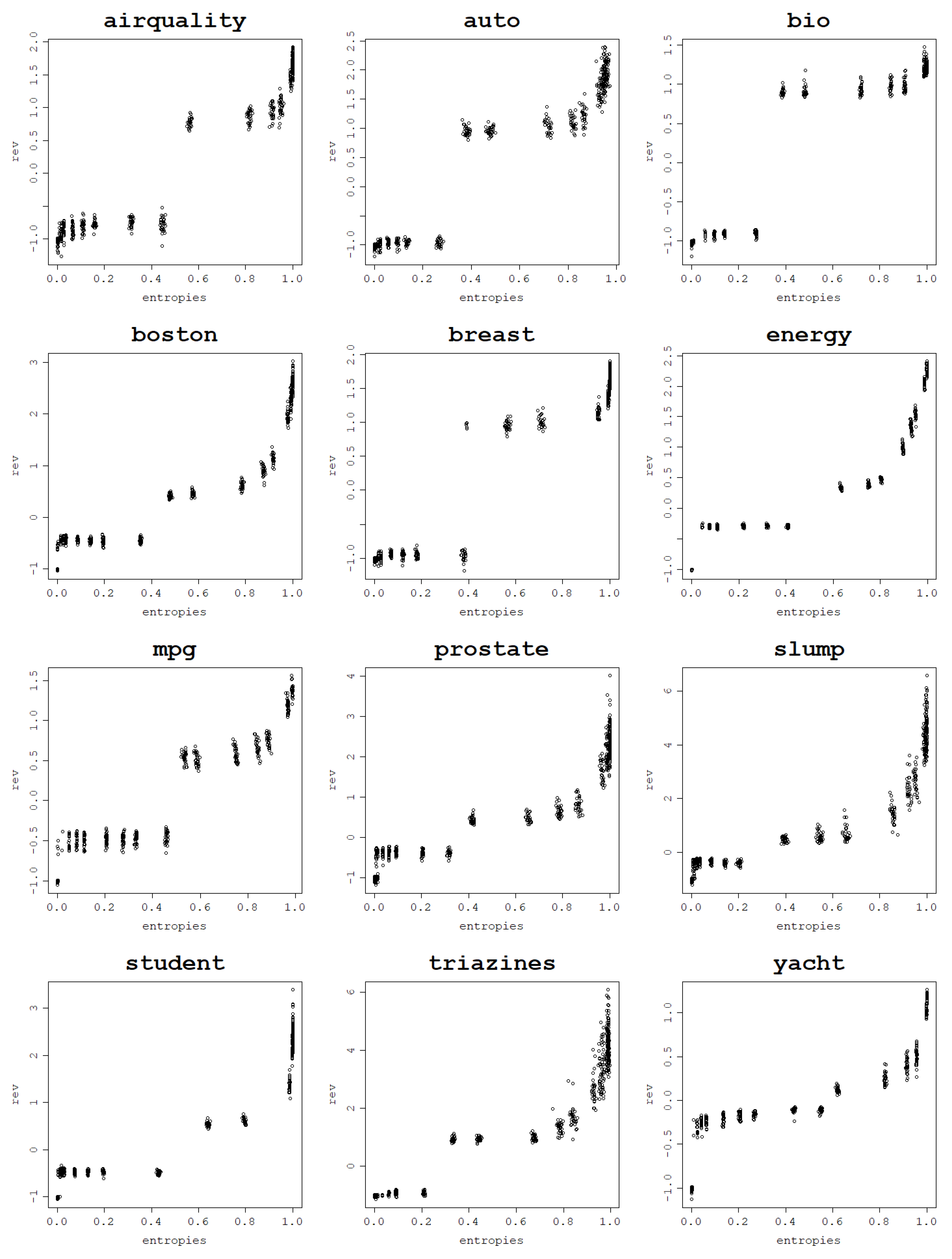
Figure 9.
Fitting ability of an RVM model with the RBF kernel: training NMSE against the von Neumann entropy across 30 train–test split folds.
Figure 9.
Fitting ability of an RVM model with the RBF kernel: training NMSE against the von Neumann entropy across 30 train–test split folds.
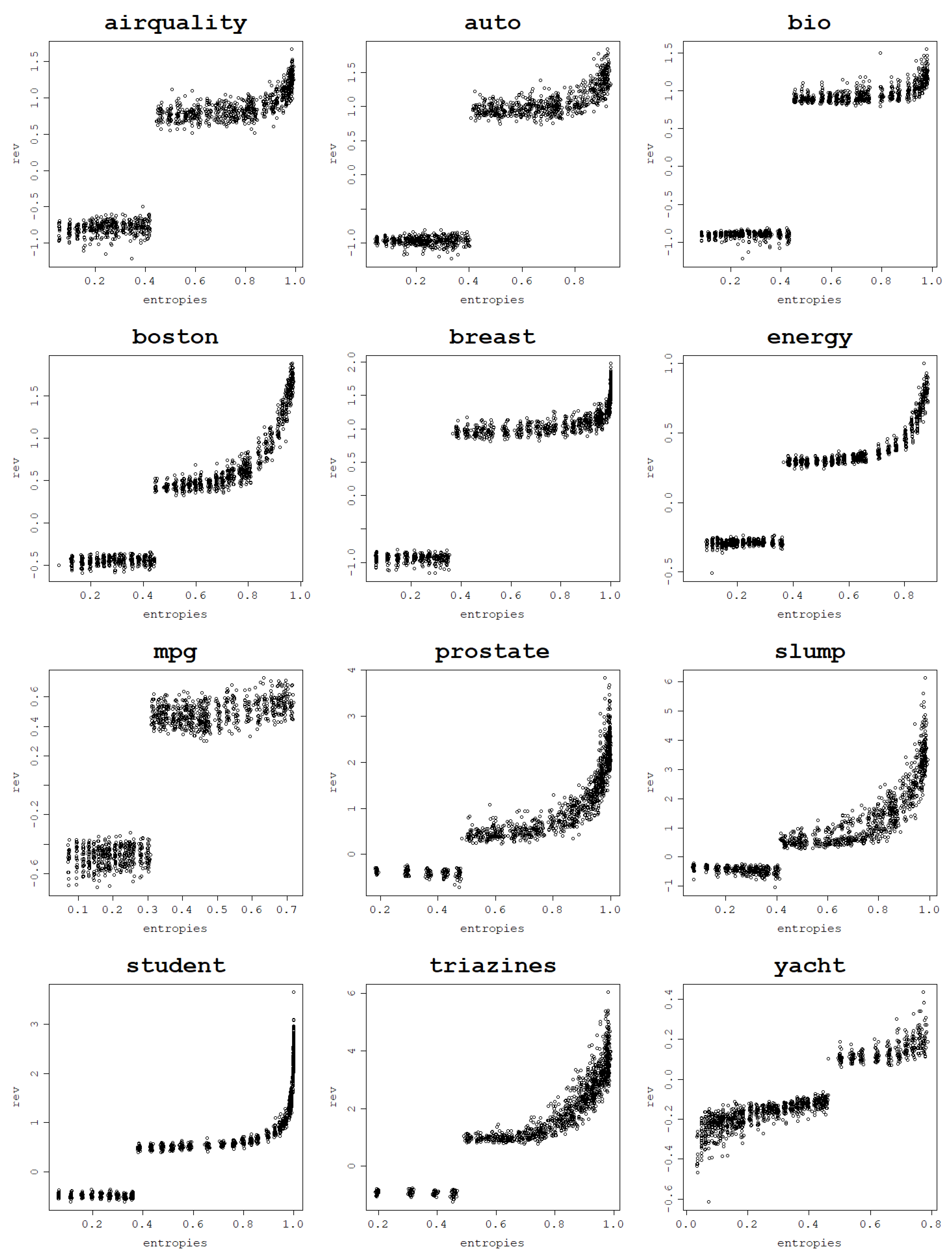
Figure 10.
Fitting ability of an RVM model with the normalized polynomial kernel: training NMSE against the von Neumann entropy across 30 train–test split folds.
Figure 10.
Fitting ability of an RVM model with the normalized polynomial kernel: training NMSE against the von Neumann entropy across 30 train–test split folds.
Figure 11.
Fitting ability of an RVM model with an ELM kernel: training NMSE against the von Neumann entropy across 30 train–test split folds.
Figure 11.
Fitting ability of an RVM model with an ELM kernel: training NMSE against the von Neumann entropy across 30 train–test split folds.
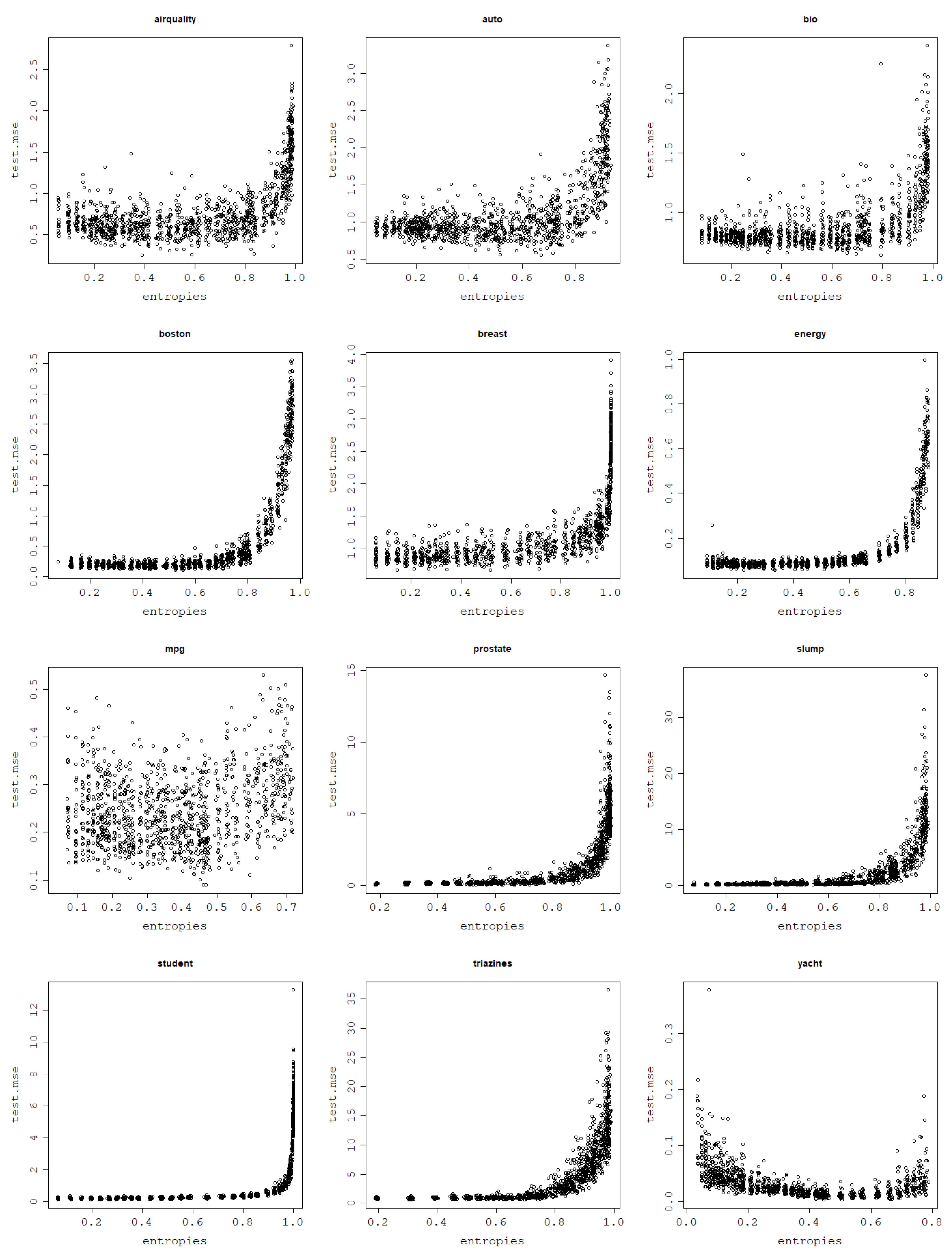
Figure 12.
Generalization power of an RVM model with the RBF kernel across 30 train–test split folds.
Figure 12.
Generalization power of an RVM model with the RBF kernel across 30 train–test split folds.
Figure 13.
Generalization power of an RVM model with the normalized polynomial kernel across 30 train–test split folds.
Figure 13.
Generalization power of an RVM model with the normalized polynomial kernel across 30 train–test split folds.
Figure 14.
Generalization power of an RVM model with the RBF kernel on a single train–test split fold and a polynomial regression of the degree 2 curve.
Figure 14.
Generalization power of an RVM model with the RBF kernel on a single train–test split fold and a polynomial regression of the degree 2 curve.
Figure 15.
Generalization power of an RVM model with the normalized polynomial kernel a on a single train–test split fold and a polynomial regression of the degree 2 curve.
Figure 15.
Generalization power of an RVM model with the normalized polynomial kernel a on a single train–test split fold and a polynomial regression of the degree 2 curve.
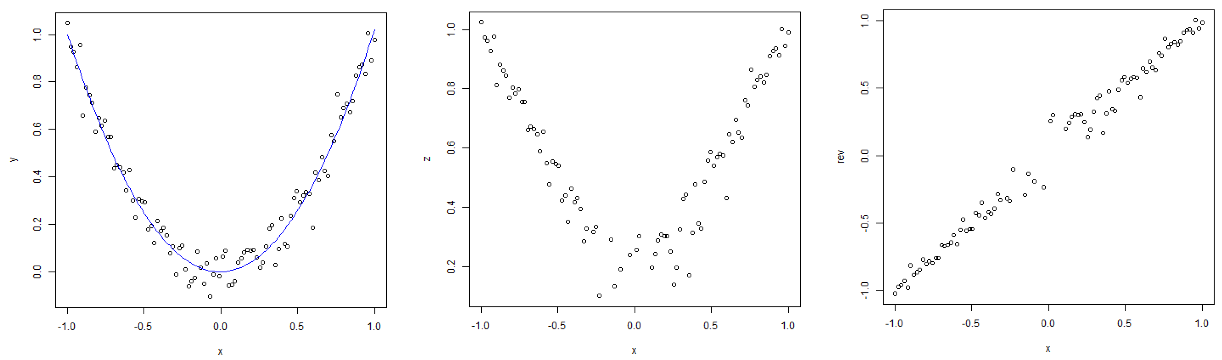
Figure 16.
Illustration of the procedure used to transform a non-monotonic relationship into a monotonic one.
Figure 16.
Illustration of the procedure used to transform a non-monotonic relationship into a monotonic one.
Figure 17.
Relationship between the von Neumann entropy and test NMSE for the RBF kernel after taking a square root and reversing the NMSE sign to the left of the minimum of the parabola.
Figure 17.
Relationship between the von Neumann entropy and test NMSE for the RBF kernel after taking a square root and reversing the NMSE sign to the left of the minimum of the parabola.
Figure 18.
Relationship between the von Neumann entropy and test NMSE for the normalized polynomial kernel after taking a square root and reversing the NMSE sign to the left of the minimum of the parabola.
Figure 18.
Relationship between the von Neumann entropy and test NMSE for the normalized polynomial kernel after taking a square root and reversing the NMSE sign to the left of the minimum of the parabola.
Figure 19.
The fitting ability of an RVM model with the RBF kernel (left) and normalized polynomial kernel (right): training NMSE against the von Neumann entropy across 5 train–test split folds.
Figure 19.
The fitting ability of an RVM model with the RBF kernel (left) and normalized polynomial kernel (right): training NMSE against the von Neumann entropy across 5 train–test split folds.
Figure 20.
Generalization power of an RVM model with the RBF kernel (left) and normalized polynomial kernel (right): test NMSE against the von Neumann entropy across 5 train–test split folds.
Figure 20.
Generalization power of an RVM model with the RBF kernel (left) and normalized polynomial kernel (right): test NMSE against the von Neumann entropy across 5 train–test split folds.
Figure 21.
Generalization power of an RVM model with the RBF kernel (left) and normalized polynomial kernel (right) on a single train–test split fold and a polynomial regression of the degree 2 curve.
Figure 21.
Generalization power of an RVM model with the RBF kernel (left) and normalized polynomial kernel (right) on a single train–test split fold and a polynomial regression of the degree 2 curve.
Figure 22.
Correlation between the von Neumann entropy and test NMSE for the RBF kernel (left) and normalized polynomial kernel (right) after taking a square root and reversing the NMSE sign to the left of the minimum of the parabola.
Figure 22.
Correlation between the von Neumann entropy and test NMSE for the RBF kernel (left) and normalized polynomial kernel (right) after taking a square root and reversing the NMSE sign to the left of the minimum of the parabola.
Table 1.
Summary of the influence of kernel parameters on the von Neumann entropy and their relation to the model’s behavior.
Table 1.
Summary of the influence of kernel parameters on the von Neumann entropy and their relation to the model’s behavior.
| |
|---|
| von Neumann entropy | von Neumann entropy |
| |
| |
| overfitting | underfitting |
| high variance | low variance |
| low bias | high bias |
Table 2.
Detailed list of datasets used for experiments along with their sizes (number of rows) and dimensionalities.
Table 2.
Detailed list of datasets used for experiments along with their sizes (number of rows) and dimensionalities.
| Dataset | Size | Dimensionality |
|---|
| auto | 205 | 26 |
| Boston | 506 | 14 |
| prostate | 97 | 10 |
| air quality | 153 | 6 |
| triazines | 186 | 59 |
| slump | 103 | 10 |
| yacht | 364 | 7 |
| energy | 768 | 9 |
| mpg | 404 | 8 |
| student | 395 | 33 |
| bio | 320 | 5 |
| breast | 198 | 33 |
Table 3.
Correlation coefficients between the von Neumann entropy and training NMSE for the RBF kernel per dataset.
Table 3.
Correlation coefficients between the von Neumann entropy and training NMSE for the RBF kernel per dataset.
| Dataset | Spearman Correlation | Pearson Correlation |
|---|
| auto | −0.809 | −0.845 |
| Boston | −0.925 | −0.598 |
| prostate | −0.873 | −0.545 |
| air quality | −0.883 | −0.831 |
| triazines | −0.821 | −0.801 |
| slump | −0.909 | −0.551 |
| yacht | −0.933 | −0.622 |
| energy | −0.947 | −0.718 |
| mpg | −0.951 | −0.75 |
| student | −0.939 | −0.699 |
| bio | −0.783 | −0.768 |
| breast | −0.846 | −0.928 |
Table 4.
Correlation coefficients between the von Neumann entropy and training NMSE for the normalized polynomial kernel per dataset.
Table 4.
Correlation coefficients between the von Neumann entropy and training NMSE for the normalized polynomial kernel per dataset.
| Dataset | Spearman Correlation | Pearson Correlation |
|---|
| auto | −0.773 | −0.75 |
| Boston | −0.962 | −0.927 |
| prostate | −0.819 | −0.758 |
| air quality | −0.86 | −0.801 |
| triazines | −0.883 | −0.795 |
| slump | −0.809 | −0.732 |
| yacht | −0.943 | −0.644 |
| energy | −0.77 | −0.691 |
| mpg | −0.8 | −0.806 |
| student | −0.963 | −0.954 |
| bio | −0.581 | −0.552 |
| breast | −0.869 | −0.841 |
Table 5.
Correlation between the von Neumann entropy and training NMSE for the ELM kernel per dataset.
Table 5.
Correlation between the von Neumann entropy and training NMSE for the ELM kernel per dataset.
| Dataset | Spearman Correlation | Pearson Correlation |
|---|
| auto | −0.652 | −0.744 |
| Boston | −0.755 | −0.986 |
| prostate | −0.82 | −0.917 |
| air quality | −0.727 | −0.9 |
| triazines | −0.593 | −0.62 |
| slump | −0.809 | −0.685 |
| yacht | −0.648 | −0.935 |
| energy | −0.745 | −0.925 |
| mpg | −0.673 | −0.903 |
| student | −0.836 | −0.966 |
| bio | −0.757 | −0.909 |
| breast | −0.396 | −0.417 |
Table 6.
Correlation between the von Neumann entropy and test NMSE for the RBF kernel after taking a square root and reversing the NMSE sign to the left of the minimum of the parabola.
Table 6.
Correlation between the von Neumann entropy and test NMSE for the RBF kernel after taking a square root and reversing the NMSE sign to the left of the minimum of the parabola.
| Dataset | Spearman Correlation | Pearson Correlation |
|---|
| auto | 0.883 | 0.968 |
| Boston | 0.954 | 0.943 |
| prostate | 0.947 | 0.95 |
| air quality | 0.934 | 0.97 |
| triazines | 0.944 | 0.947 |
| slump | 0.956 | 0.932 |
| yacht | 0.949 | 0.912 |
| energy | 0.957 | 0.943 |
| mpg | 0.942 | 0.960 |
| student | 0.934 | 0.958 |
| bio | 0.927 | 0.951 |
| breast | 0.892 | 0.976 |
Table 7.
Correlation between the von Neumann entropy and test NMSE for the normalized polynomial kernel after taking a square root and reversing the NMSE sign to the left of the minimum of the parabola.
Table 7.
Correlation between the von Neumann entropy and test NMSE for the normalized polynomial kernel after taking a square root and reversing the NMSE sign to the left of the minimum of the parabola.
| Dataset | Spearman Correlation | Pearson Correlation |
|---|
| auto | 0.881 | 0.903 |
| Boston | 0.945 | 0.943 |
| prostate | 0.954 | 0.869 |
| air quality | 0.9 | 0.916 |
| triazines | 0.953 | 0.906 |
| slump | 0.938 | 0.877 |
| yacht | 0.926 | 0.927 |
| energy | 0.926 | 0.938 |
| mpg | 0.804 | 0.842 |
| student | 0.973 | 0.869 |
| bio | 0.876 | 0.884 |
| breast | 0.939 | 0.891 |
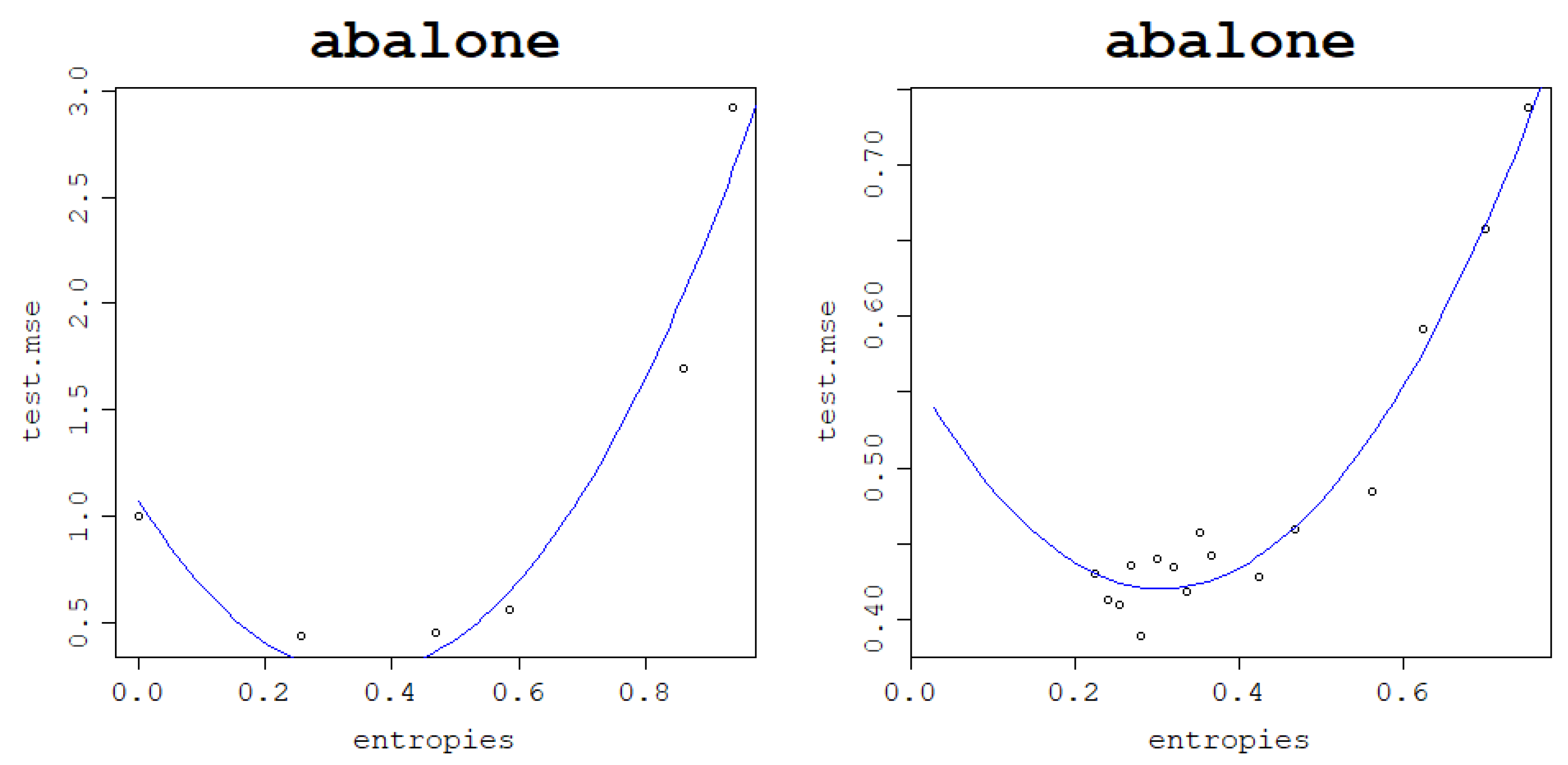
Table 8.
Heuristic for the optimal von Neumann entropy for the RBF kernel defined as the minimum of the parabola resulting from the modeling of the test NMSE against the von Neumann entropy as a degree 2 polynomial regression.
Table 8.
Heuristic for the optimal von Neumann entropy for the RBF kernel defined as the minimum of the parabola resulting from the modeling of the test NMSE against the von Neumann entropy as a degree 2 polynomial regression.
| Dataset | von Neumann Entropy |
|---|
| auto | 0.343 |
| Boston | 0.416 |
| prostate | 0.396 |
| air quality | 0.481 |
| triazines | 0.315 |
| slump | 0.331 |
| yacht | 0.557 |
| energy | 0.413 |
| mpg | 0.471 |
| student | 0.449 |
| bio | 0.372 |
| breast | 0.389 |
Table 9.
Heuristic for the optimal von Neumann entropy for the normalized polynomial kernel defined as the minimum of the parabola resulting from modeling the test NMSE against the von Neumann entropy as a degree 2 polynomial regression.
Table 9.
Heuristic for the optimal von Neumann entropy for the normalized polynomial kernel defined as the minimum of the parabola resulting from modeling the test NMSE against the von Neumann entropy as a degree 2 polynomial regression.
| Dataset | von Neumann Entropy |
|---|
| auto | 0.401 |
| Boston | 0.444 |
| prostate | 0.480 |
| air quality | 0.421 |
| triazines | 0.489 |
| slump | 0.413 |
| yacht | 0.463 |
| energy | 0.363 |
| mpg | 0.309 |
| student | 0.362 |
| bio | 0.439 |
| breast | 0.359 |
Table 10.
Comparison of the heuristic and optimal results for the RBF kernel. From third column onwards: heuristic , heuristic vNe, optimal NMSE, heuristic NMSE, optimal number of tries for , heuristic number of tries for .
Table 10.
Comparison of the heuristic and optimal results for the RBF kernel. From third column onwards: heuristic , heuristic vNe, optimal NMSE, heuristic NMSE, optimal number of tries for , heuristic number of tries for .
| Data | | heu. | heu.vNe | opt.nmse | heu.nmse | opt.#tried | heu.#tried |
|---|
| auto | 0.3 | 8.554 | 0.451 | 0.905 | 0.906 | 24 | 5 |
| Boston | 6 | 5.669 | 0.468 | 0.174 | 0.176 | 24 | 7 |
| prostate | 0.1 | 1 | 0.418 | 0.143 | 0.194 | 24 | 1 |
| air quality | 3 | 5.669 | 0.439 | 0.559 | 0.618 | 24 | 7 |
| triazines | 0.1 | 1 | 0.442 | 0.851 | 0.879 | 24 | 1 |
| slump | 0.3 | 3.885 | 0.449 | 0.136 | 0.315 | 24 | 9 |
| yacht | 66 | 33 | 0.435 | 0.012 | 0.015 | 24 | 2 |
| energy | 6 | 13.223 | 0.459 | 0.082 | 0.086 | 24 | 3 |
| mpg | 33 | 33 | 0.457 | 0.213 | 0.213 | 24 | 2 |
| student | 0.06 | 2.783 | 0.409 | 0.219 | 0.233 | 24 | 11 |
| bio | 3 | 8.554 | 0.453 | 0.807 | 0.796 | 24 | 5 |
| breast | 0.3 | 3.885 | 0.444 | 0.879 | 0.897 | 24 | 9 |
| average | | | 0.444 | 0.415 | 0.442 | 24 | 5.17 |
Table 11.
Comparison of the heuristic and optimal results for the normalized polynomial kernel.
Table 11.
Comparison of the heuristic and optimal results for the normalized polynomial kernel.
| Data | d | heu. d | heu.vNe | opt.nmse | heu.nmse | opt.# dtried | heu.# dtried |
|---|
| auto | 50 | 31.175 | 0.433 | 0.878 | 0.913 | 46 | 3 |
| Boston | 25 | 19.649 | 0.442 | 0.186 | 0.188 | 46 | 5 |
| prostate | 1 | 3.721 | 0.410 | 0.128 | 0.194 | 46 | 13 |
| air quality | 9 | 19.649 | 0.41 | 0.582 | 0.616 | 46 | 5 |
| triazines | 2 | 3.721 | 0.44 | 0.858 | 0.899 | 46 | 3 |
| slump | 2 | 12.526 | 0.405 | 0.127 | 0.269 | 46 | 7 |
| yacht | 200 | 80 | 0.361 | 0.012 | 0.02 | 46 | 2 |
| energy | 20 | 31.175 | 0.364 | 0.08 | 0.085 | 46 | 3 |
| mpg | 60 | 80 | 0.404 | 0.206 | 0.208 | 46 | 2 |
| student | 3 | 12.526 | 0.444 | 0.223 | 0.242 | 46 | 7 |
| bio | 50 | 31.175 | 0.435 | 0.777 | 0.795 | 46 | 3 |
| breast | 4 | 12.526 | 0.392 | 0.853 | 0.898 | 46 | 7 |
| average | | | 0.412 | 0.41 | 0.444 | 46 | 5 |
Table 12.
Correlation between the von Neumann entropy and training NMSE for the RBF kernel and normalized polynomial kernel for the Abalone dataset.
Table 12.
Correlation between the von Neumann entropy and training NMSE for the RBF kernel and normalized polynomial kernel for the Abalone dataset.
| Dataset | Kernel | Spearman Correlation | Pearson Correlation |
|---|
| abalone | RBF | −0.986 | −0.926 |
| abalone | normalized polynomial | −0.889 | −0.954 |
Table 13.
Correlation between the von Neumann entropy and test NMSE for the RBF kernel and normalized polynomial kernel for the Abalone dataset.
Table 13.
Correlation between the von Neumann entropy and test NMSE for the RBF kernel and normalized polynomial kernel for the Abalone dataset.
| Dataset | Kernel | Spearman Correlation | Pearson Correlation |
|---|
| abalone | RBF | 0.98 | 0.94 |
| abalone | normalized polynomial | 0.90 | 0.78 |
Table 14.
Comparison of the RBF kernel optimal results with the heuristic ones for the Abalone dataset.
Table 14.
Comparison of the RBF kernel optimal results with the heuristic ones for the Abalone dataset.
| Dataset | | heu. | heu.vNe | opt.nmse | heu.nmse | opt.#tried | heu.#tried |
|---|
| abalone | 10 | 33 | 0.406 | 0.422 | 0.44 | 16 | 2 |
Table 15.
Comparison of the normalized polynomial kernel optimal results with the heuristic ones for the Abalone dataset.
Table 15.
Comparison of the normalized polynomial kernel optimal results with the heuristic ones for the Abalone dataset.
| Dataset | d | heu.d | heu.vNe | opt.nmse | heu.nmse | opt.#dtried | heu.#dtried |
|---|
| abalone | 50 | 70 | 0.32 | 0.42 | 0.443 | 32 | 2 |


