

Pairing Optimization via Statistics: Algebraic Structure in Pairing Problems and Its Application to Performance Enhancement
 , , , , , and
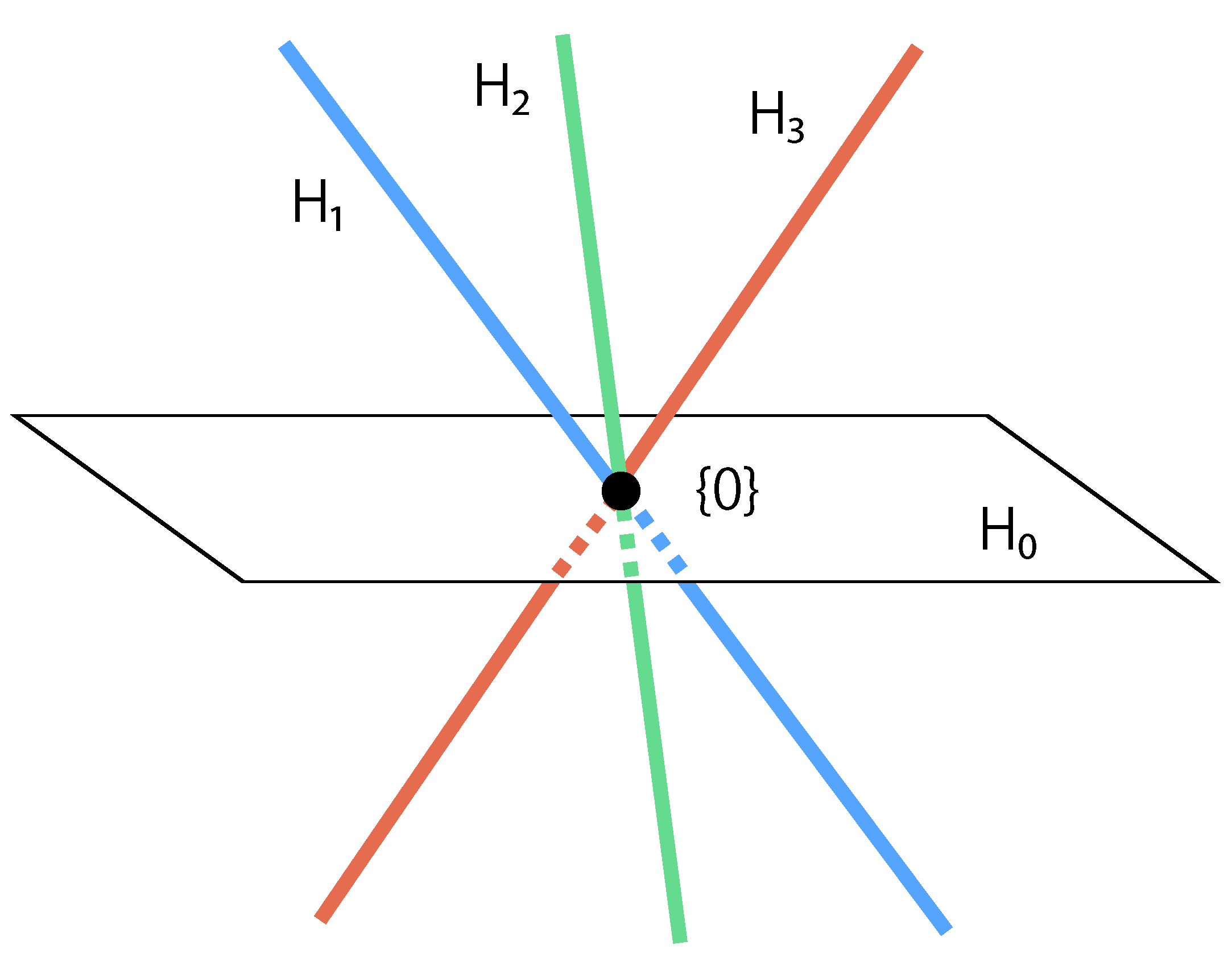
Abstract
:1. Introduction
2. Problem Setting
2.1. Pairing Optimization Problem
2.2. Limited Observation Constraint
3. Mathematical Properties of the Pairing Problem
3.1. Adjacent Set
3.2. Equivalence Class
3.3. Mean and Covariance
4. Variance Optimization
4.1. Performance Degradation through the Observation Phase
4.2. Transforming the Compatibility Matrix with Minimized Variance
5. Simulation
5.1. Setting
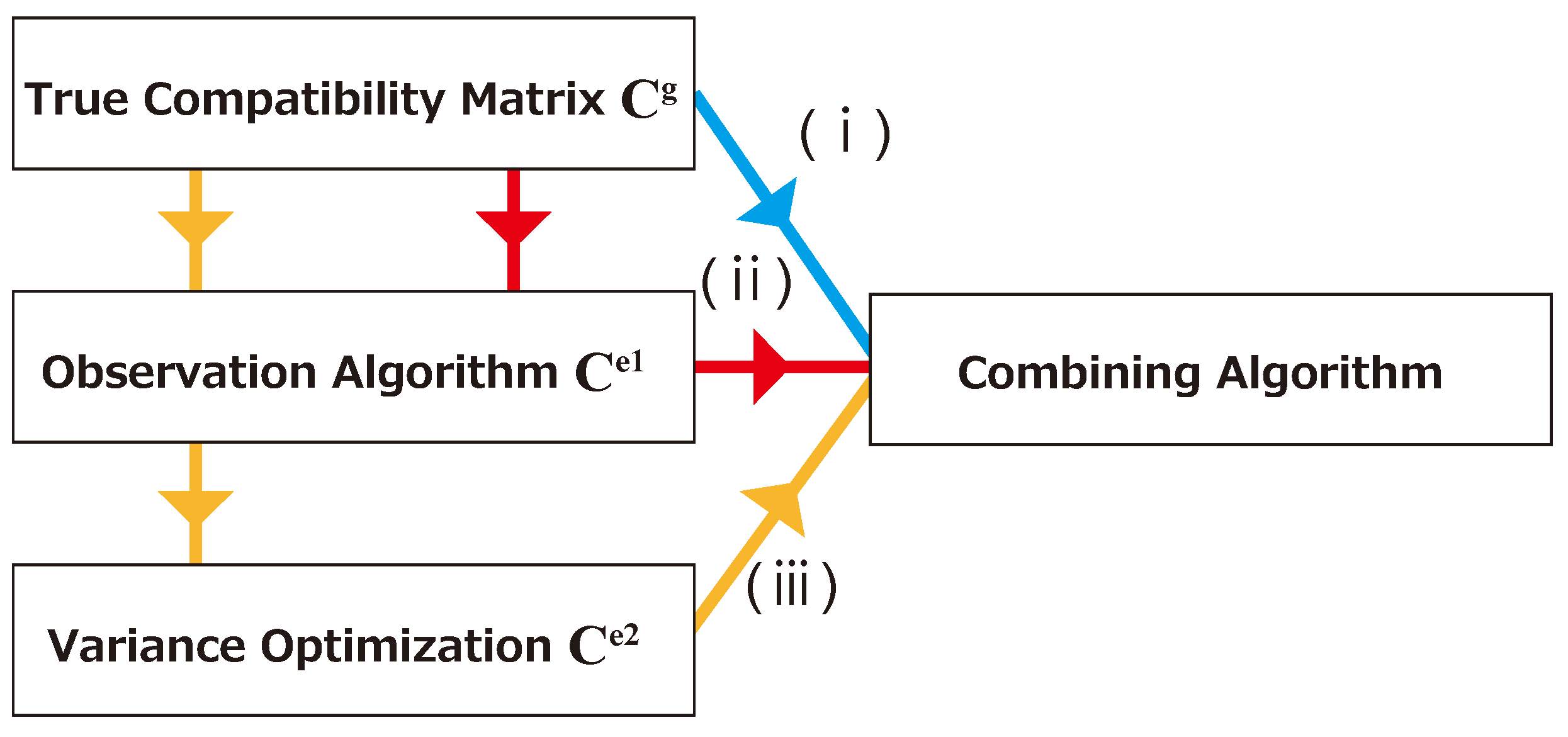
5.2. Simulation Flow
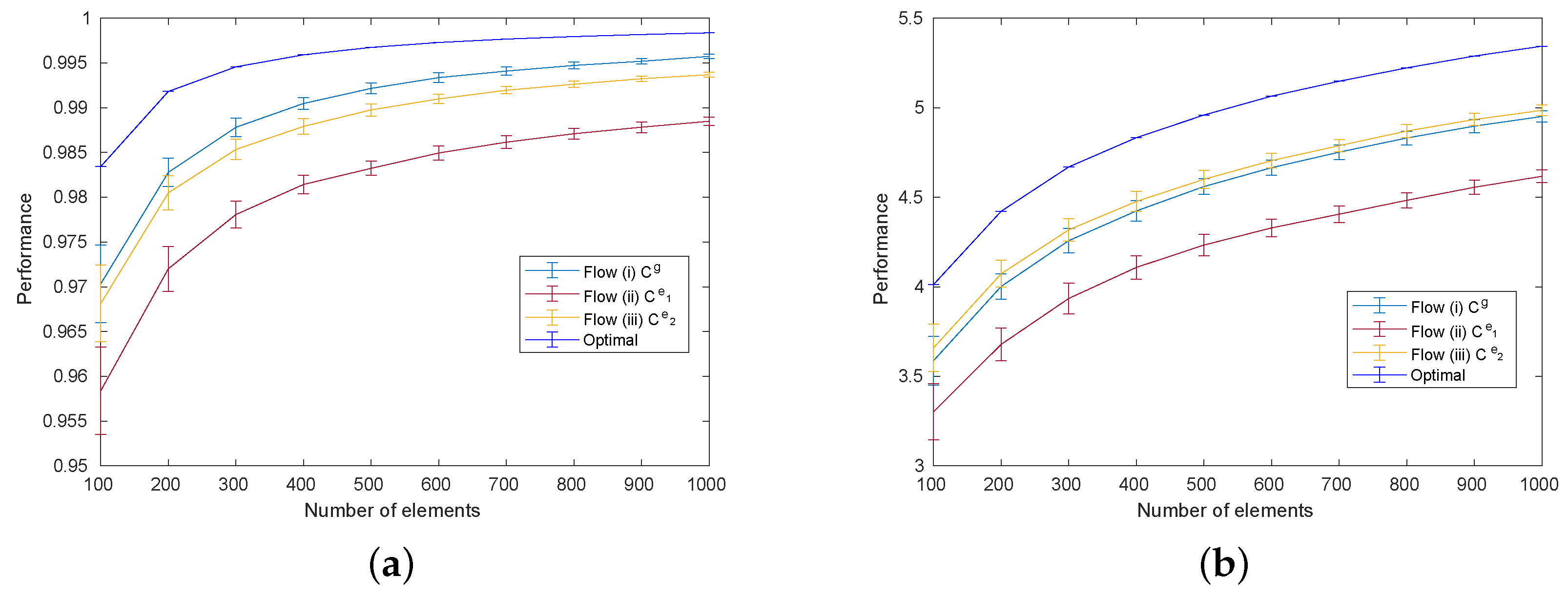
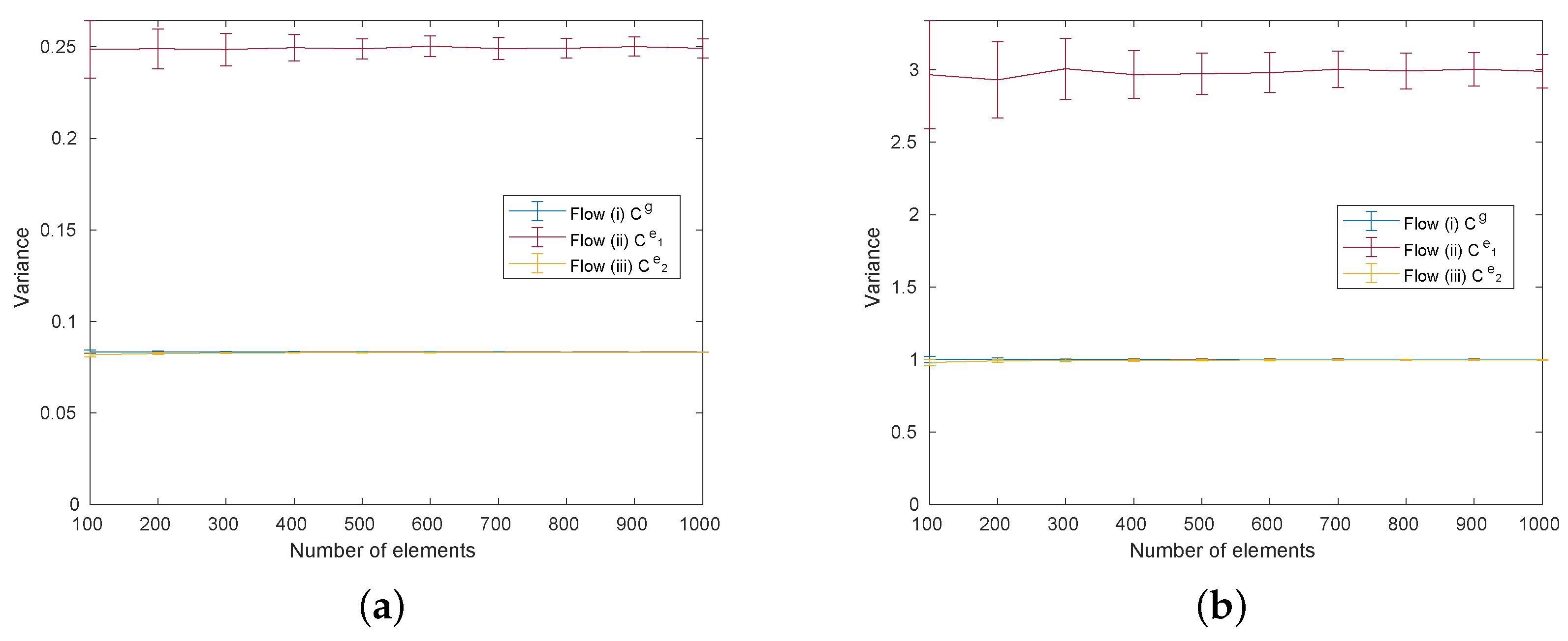
5.3. Performance
6. Conclusions
Author Contributions
Funding
Institutional Review Board Statement
Informed Consent Statement
Data Availability Statement
Acknowledgments
Conflicts of Interest
Appendix A. Matrix Form of Conserved Quantities
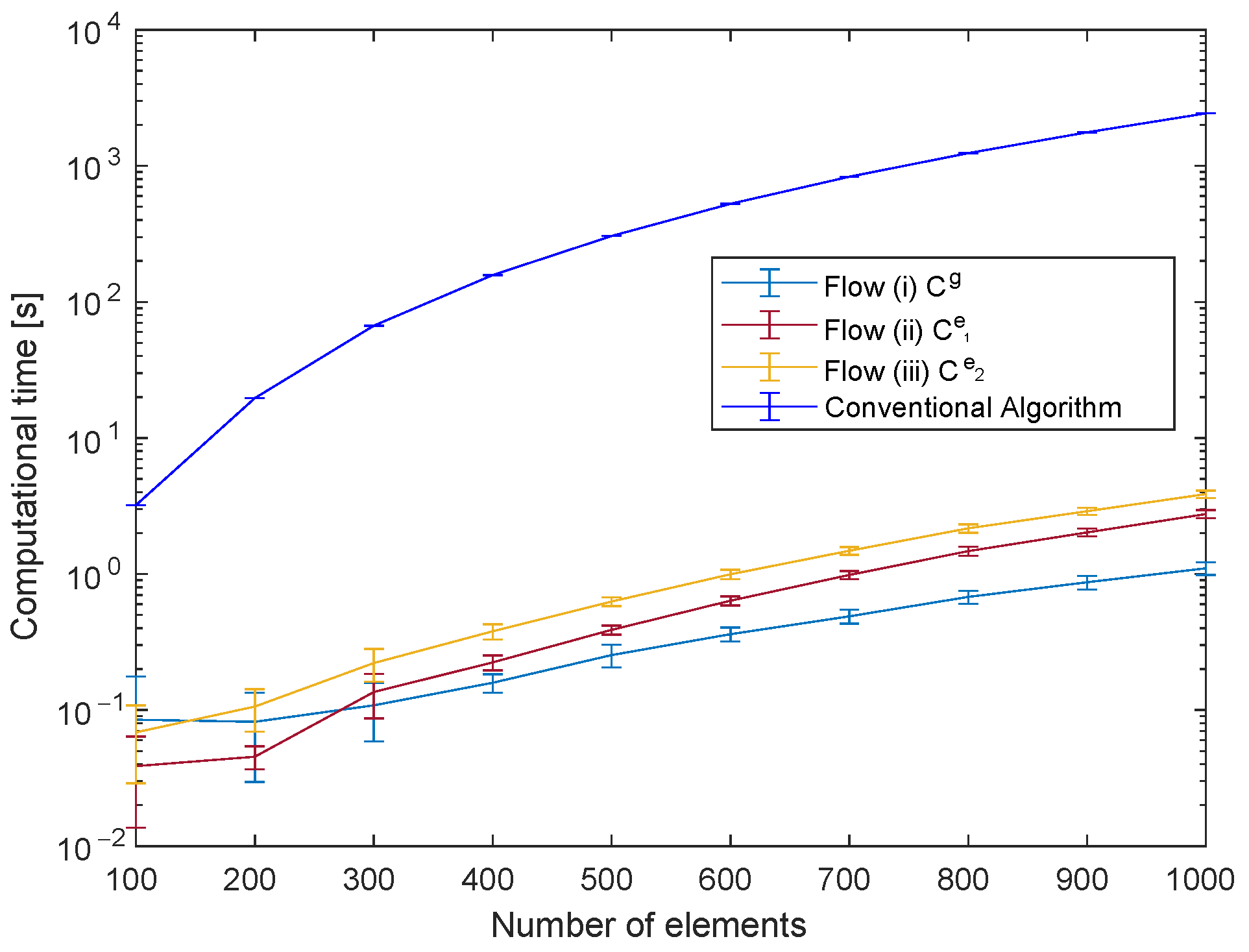
Appendix B. Computational Time

References
- Gale, D.; Shapley, L.S. College admissions and the stability of marriage. Am. Math. Mon. 1962, 69, 9–15. [Google Scholar] [CrossRef]
- Roth, A.E. The economics of matching: Stability and incentives. Math. Oper. Res. 1982, 7, 617–628. [Google Scholar] [CrossRef] [Green Version]
- Ergin, H.; Sönmez, T.; Ünver, M.U. Dual-Donor Organ Exchange. Econometrica 2017, 85, 1645–1671. [Google Scholar] [CrossRef] [Green Version]
- Kohl, N.; Karisch, S.E. Airline crew rostering: Problem types, modeling, and optimization. Ann. Oper. Res. 2004, 127, 223–257. [Google Scholar] [CrossRef]
- Gambetta, J.M.; Chow, J.M.; Steffen, M. Building logical qubits in a superconducting quantum computing system. npj Quantum Inf. 2017, 3, 1–7. [Google Scholar] [CrossRef] [Green Version]
- Gao, Y.; Dai, Q.; Wang, M.; Zhang, N. 3D model retrieval using weighted bipartite graph matching. Signal Process. Image Commun. 2011, 26, 39–47. [Google Scholar] [CrossRef]
- Bellur, U.; Kulkarni, R. Improved matchmaking algorithm for semantic web services based on bipartite graph matching. In Proceedings of the IEEE International Conference on Web Services (ICWS 2007), Salt Lake City, UT, USA, 9–13 July 2007; pp. 86–93. [Google Scholar]
- Edmonds, J. Paths, trees, and flowers. Can. J. Math. 1965, 17, 449–467. [Google Scholar] [CrossRef]
- Gabow, H.N. Data structures for weighted matching and nearest common ancestors with linking. In Proceedings of the First Annual ACM-SIAM Symposium on Discrete Algorithms, San Francisco, CA, USA, 22–24 January 1990; pp. 434–443. [Google Scholar]
- Huang, C.C.; Kavitha, T. Efficient algorithms for maximum weight matchings in general graphs with small edge weights. In Proceedings of the Twenty-Third Annual ACM-SIAM Symposium on Discrete Algorithms, Kyoto, Japan, 17–19 January 2012; pp. 1400–1412. [Google Scholar]
- Pettie, S. A simple reduction from maximum weight matching to maximum cardinality matching. Inf. Process. Lett. 2012, 112, 893–898. [Google Scholar] [CrossRef] [Green Version]
- Cygan, M.; Gabow, H.N.; Sankowski, P. Algorithmic applications of baur-strassen’s theorem: Shortest cycles, diameter, and matchings. J. ACM (JACM) 2015, 62, 1–30. [Google Scholar] [CrossRef]
- Duan, R.; Pettie, S. Approximating maximum weight matching in near-linear time. In Proceedings of the 2010 IEEE 51st Annual Symposium on Foundations of Computer Science, Las Vegas, NV, USA, 23–26 October 2010; pp. 673–682. [Google Scholar]
- Hanke, S.; Hougardy, S. New Approximation Algorithms for the Weighted Matching Problem. Citeseer. 2010. Available online: https://citeseerx.ist.psu.edu/document?repid=rep1&type=pdf&doi=f6bc65fe193c8afd779f2867831a869c59554661 (accessed on 10 January 2023).
- Duan, R.; Pettie, S. Linear-time approximation for maximum weight matching. J. Acm (JACM) 2014, 61, 1–23. [Google Scholar] [CrossRef]
- Wu, B.; Li, L. Solving maximum weighted matching on large graphs with deep reinforcement learning. Inf. Sci. 2022, 614, 400–415. [Google Scholar] [CrossRef]
- Fujita, N.; Chauvet, N.; Röhm, A.; Horisaki, R.; Li, A.; Hasegawa, M.; Naruse, M. Efficient Pairing in Unknown Environments: Minimal Observations and TSP-based Optimization. IEEE Access 2022, 10, 57630–57640. [Google Scholar] [CrossRef]
- Williams, V.V. Multiplying matrices faster than Coppersmith-Winograd. In Proceedings of the Forty-Fourth Annual ACM Symposium on Theory of Computing, New York, NY, USA, 20–22 May 2012; pp. 887–898. [Google Scholar]
- Kuhn, H.W. The Hungarian method for the assignment problem. Nav. Res. Logist. Q. 1955, 2, 83–97. [Google Scholar] [CrossRef] [Green Version]
- Bertsekas, D.P. The auction algorithm: A distributed relaxation method for the assignment problem. Ann. Oper. Res. 1988, 14, 105–123. [Google Scholar] [CrossRef] [Green Version]
- Munkres, J. Algorithms for the assignment and transportation problems. J. Soc. Ind. Appl. Math. 1957, 5, 32–38. [Google Scholar] [CrossRef] [Green Version]
- Goldberg, A.; Radzik, T. A Heuristic Improvement of the Bellman-Ford Algorithm; Technical Report; STANFORD UNIV CA DEPT OF COMPUTER SCIENCE: Stanford, CA, USA, 1993. [Google Scholar]
- Aldababsa, M.; Toka, M.; Gökçeli, S.; Kurt, G.K.; Kucur, O. A tutorial on nonorthogonal multiple access for 5G and beyond. Wirel. Commun. Mob. Comput. 2018, 2018, 9713450. [Google Scholar] [CrossRef] [Green Version]
- Ding, Z.; Fan, P.; Poor, H.V. Impact of user pairing on 5G nonorthogonal multiple-access downlink transmissions. IEEE Trans. Veh. Technol. 2015, 65, 6010–6023. [Google Scholar] [CrossRef]
- Chen, L.; Ma, L.; Xu, Y. Proportional fairness-based user pairing and power allocation algorithm for non-orthogonal multiple access system. IEEE Access 2019, 7, 19602–19615. [Google Scholar] [CrossRef]
- Ali, Z.; Khan, W.U.; Ihsan, A.; Waqar, O.; Sidhu, G.A.S.; Kumar, N. Optimizing resource allocation for 6G NOMA-enabled cooperative vehicular networks. IEEE Open J. Intell. Transp. Syst. 2021, 2, 269–281. [Google Scholar] [CrossRef]
- Zhang, H.; Duan, Y.; Long, K.; Leung, V.C. Energy efficient resource allocation in terahertz downlink NOMA systems. IEEE Trans. Commun. 2020, 69, 1375–1384. [Google Scholar] [CrossRef]
- Shahab, M.B.; Irfan, M.; Kader, M.F.; Young Shin, S. User pairing schemes for capacity maximization in non-orthogonal multiple access systems. Wirel. Commun. Mob. Comput. 2016, 16, 2884–2894. [Google Scholar] [CrossRef] [Green Version]
- Zhu, L.; Zhang, J.; Xiao, Z.; Cao, X.; Wu, D.O. Optimal user pairing for downlink non-orthogonal multiple access (NOMA). IEEE Wirel. Commun. Lett. 2018, 8, 328–331. [Google Scholar] [CrossRef]
- Higuchi, K.; Benjebbour, A. Non-orthogonal multiple access (NOMA) with successive interference cancellation for future radio access. IEICE Trans. Commun. 2015, 98, 403–414. [Google Scholar] [CrossRef] [Green Version]
- Halim, A.H.; Ismail, I. Combinatorial optimization: Comparison of heuristic algorithms in travelling salesman problem. Arch. Comput. Methods Eng. 2019, 26, 367–380. [Google Scholar] [CrossRef]
- Galil, Z. Efficient algorithms for finding maximum matching in graphs. ACM Comput. Surv. (CSUR) 1986, 18, 23–38. [Google Scholar] [CrossRef]


Disclaimer/Publisher’s Note: The statements, opinions and data contained in all publications are solely those of the individual author(s) and contributor(s) and not of MDPI and/or the editor(s). MDPI and/or the editor(s) disclaim responsibility for any injury to people or property resulting from any ideas, methods, instructions or products referred to in the content. |
© 2023 by the authors. Licensee MDPI, Basel, Switzerland. This article is an open access article distributed under the terms and conditions of the Creative Commons Attribution (CC BY) license (https://creativecommons.org/licenses/by/4.0/).
Share and Cite
Fujita, N.; Röhm, A.; Mihana, T.; Horisaki, R.; Li, A.; Hasegawa, M.; Naruse, M. Pairing Optimization via Statistics: Algebraic Structure in Pairing Problems and Its Application to Performance Enhancement. Entropy 2023, 25, 146. https://doi.org/10.3390/e25010146
Fujita N, Röhm A, Mihana T, Horisaki R, Li A, Hasegawa M, Naruse M. Pairing Optimization via Statistics: Algebraic Structure in Pairing Problems and Its Application to Performance Enhancement. Entropy. 2023; 25(1):146. https://doi.org/10.3390/e25010146
Chicago/Turabian StyleFujita, Naoki, André Röhm, Takatomo Mihana, Ryoichi Horisaki, Aohan Li, Mikio Hasegawa, and Makoto Naruse. 2023. "Pairing Optimization via Statistics: Algebraic Structure in Pairing Problems and Its Application to Performance Enhancement" Entropy 25, no. 1: 146. https://doi.org/10.3390/e25010146