


Cross-Subject Emotion Recognition Using Fused Entropy Features of EEG


Abstract
:1. Introduction
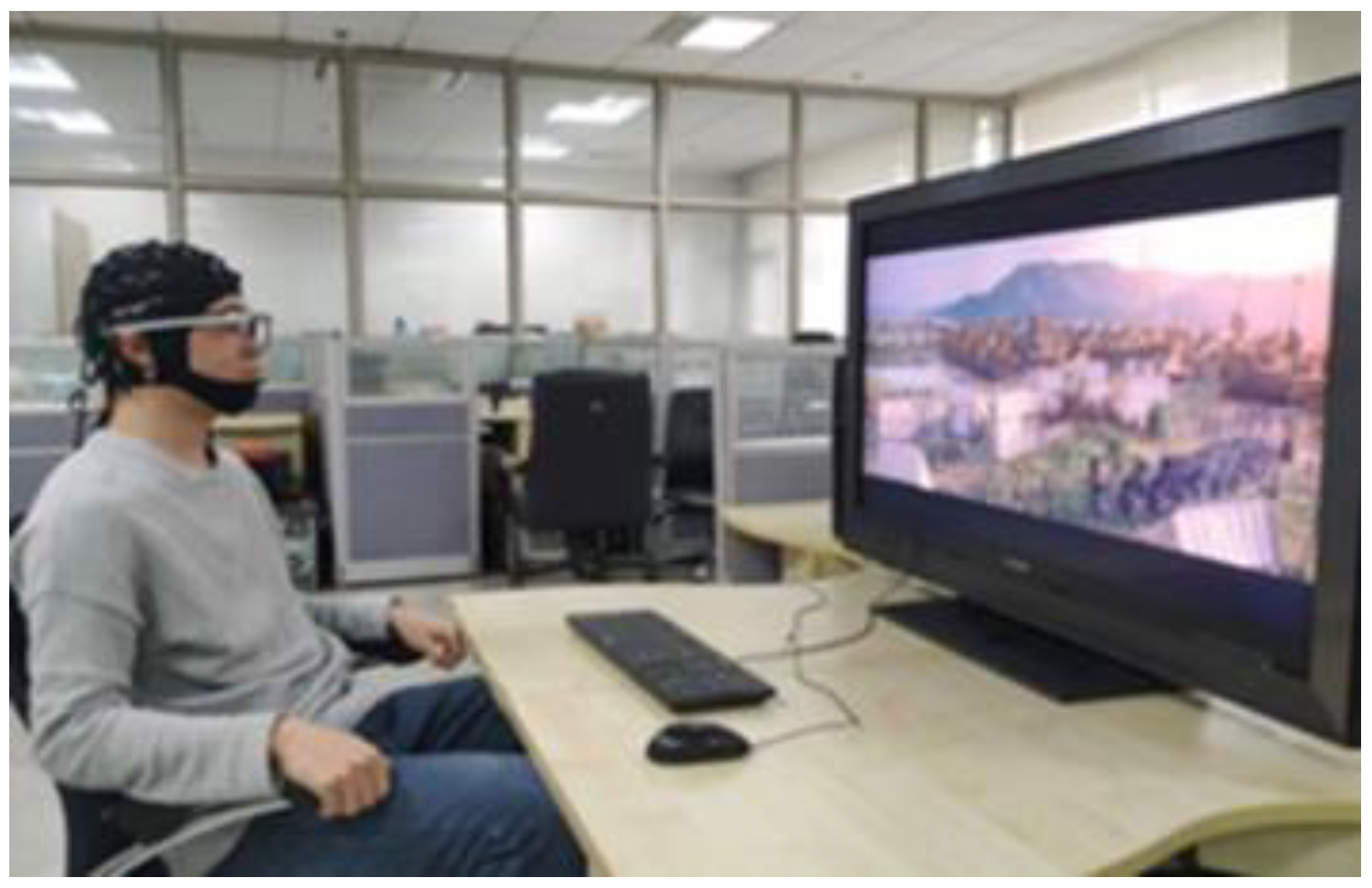
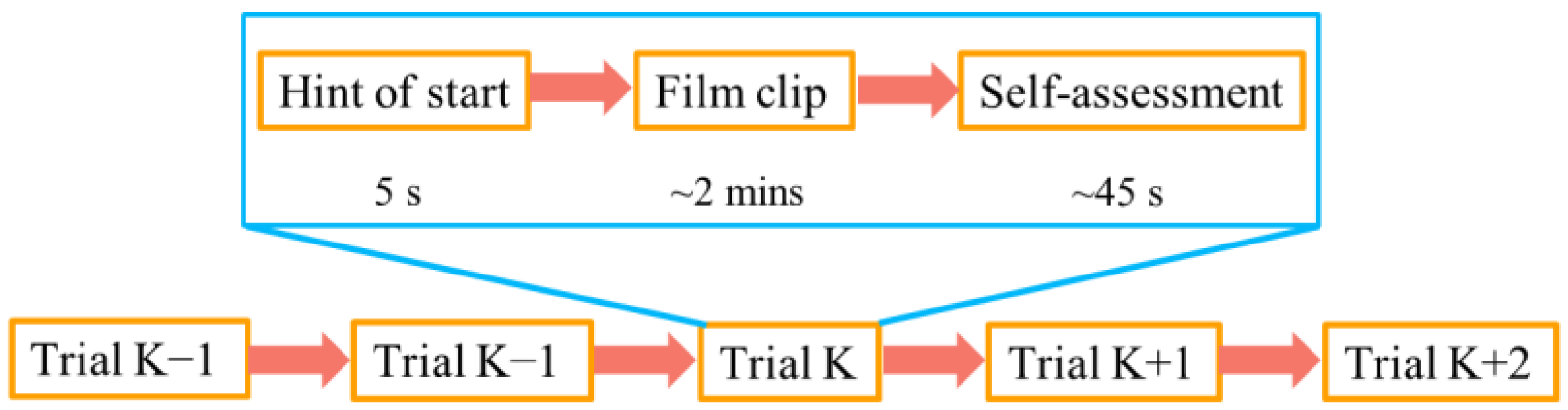
2. Data Resource
3. Methodology
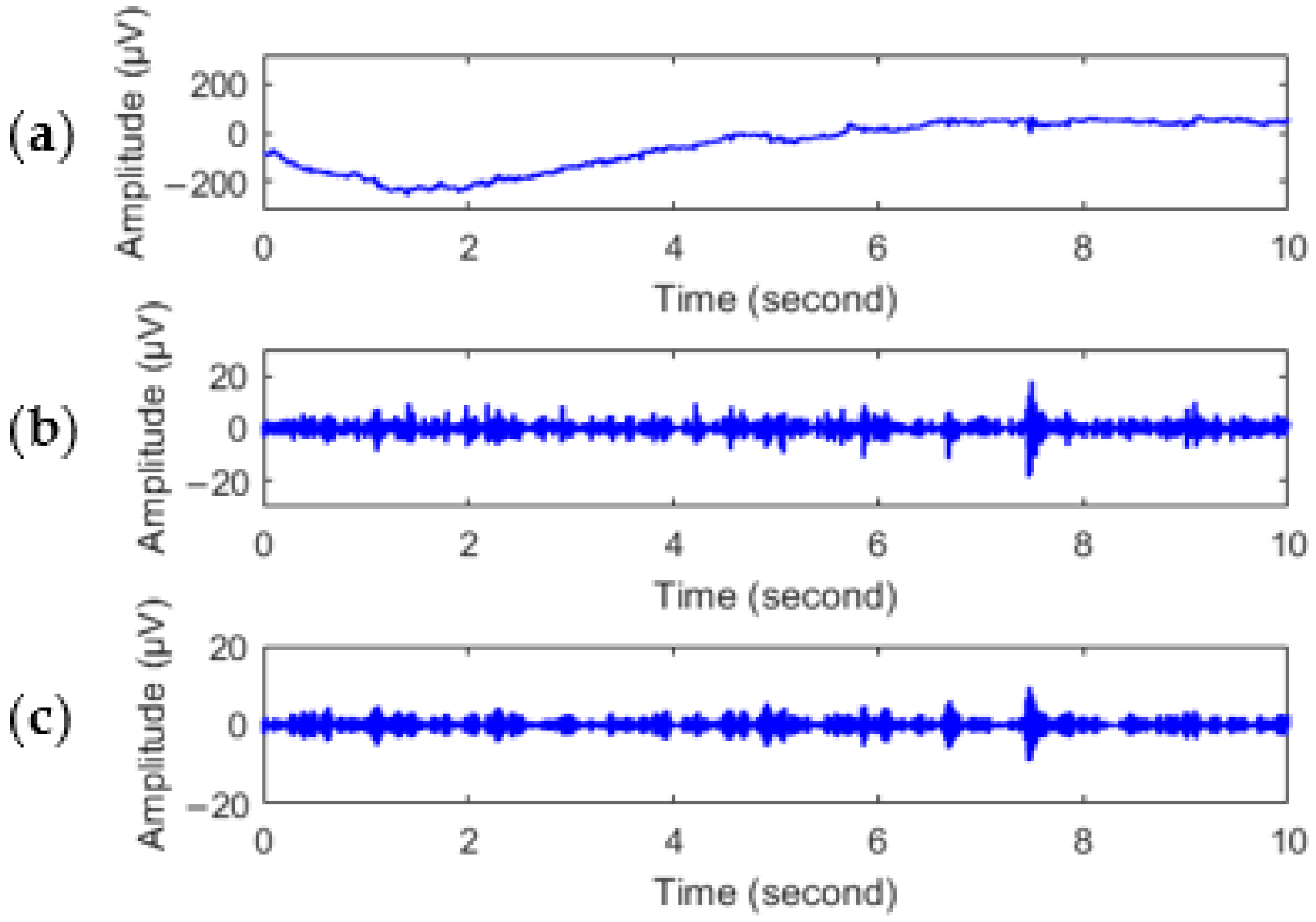
3.1. Preprocessing
3.2. Feature Extraction
3.2.1. Multi-Scale Entropy
3.2.2. Approximate Entropy
3.2.3. Fuzzy Entropy
3.2.4. Rényi Entropy
3.2.5. Differential Entropy
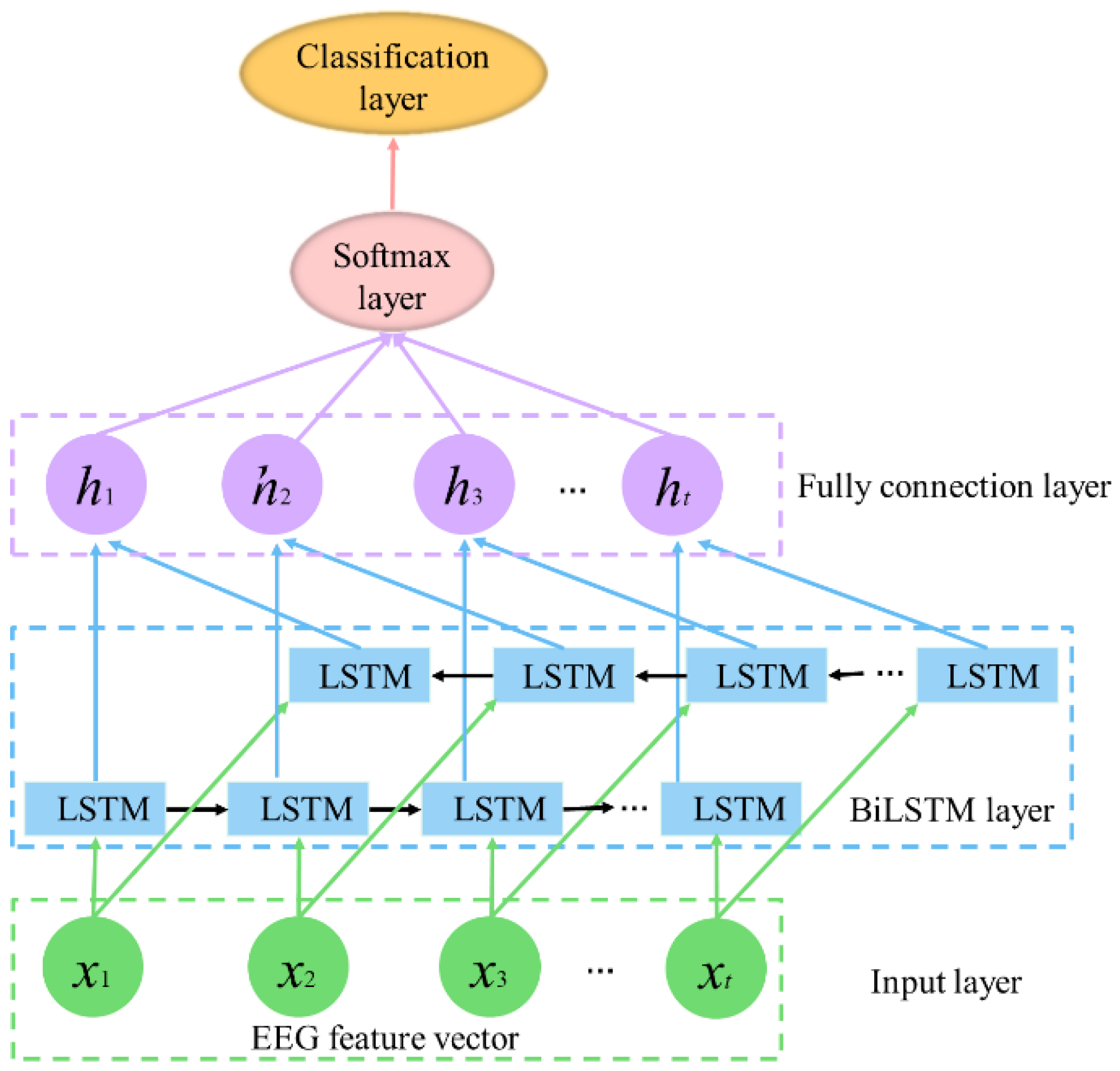
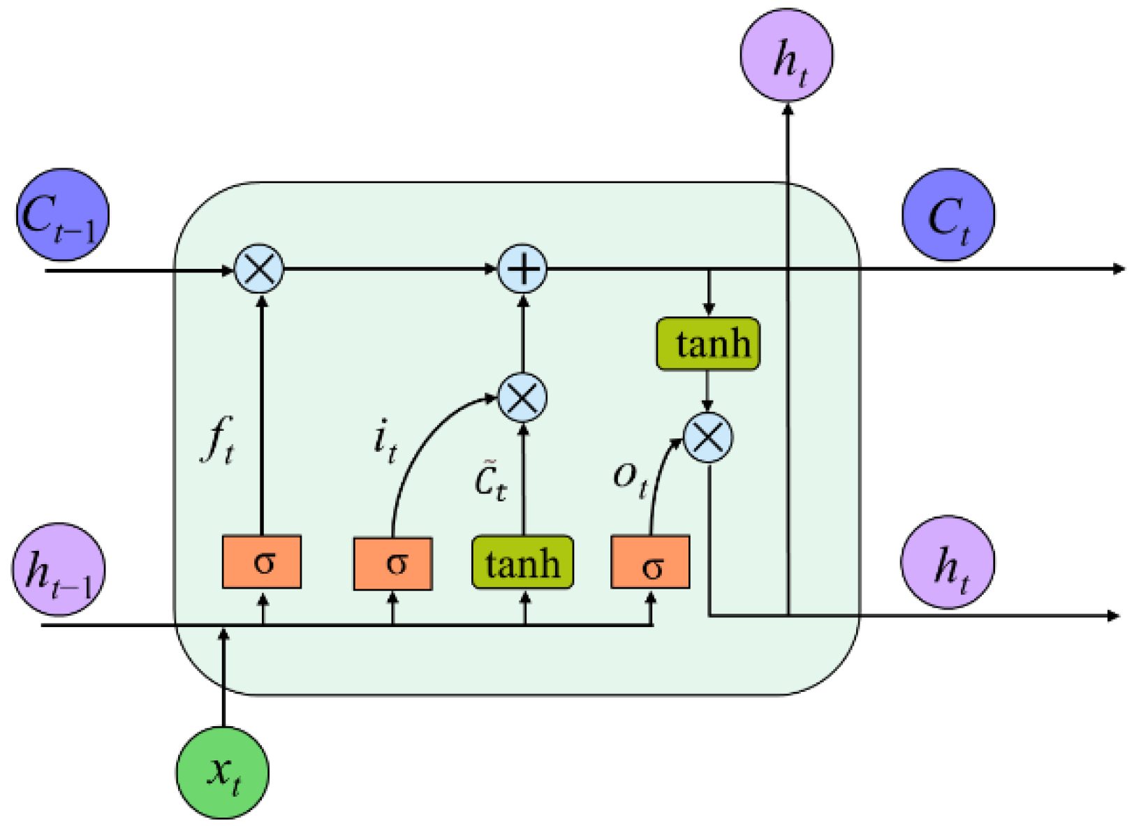
3.3. BiLSTM
4. Results
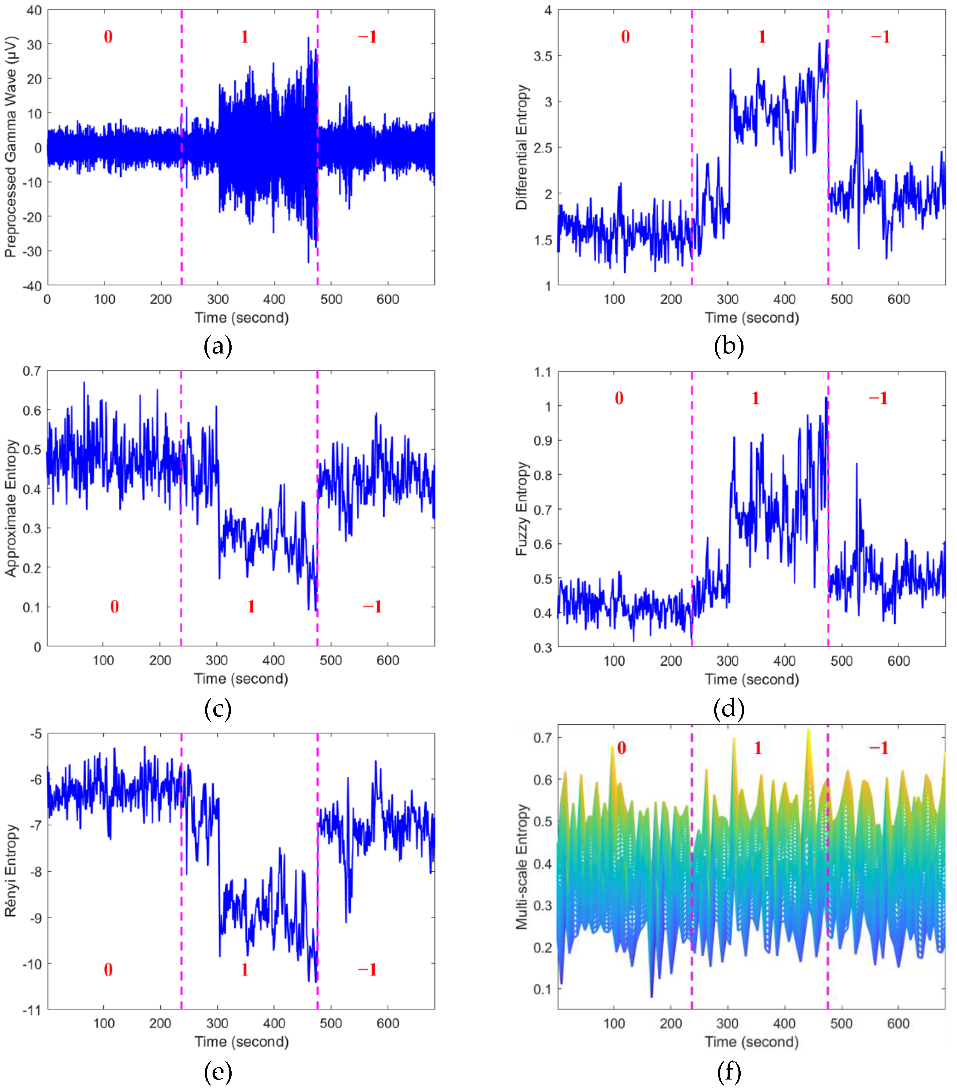
4.1. Feature Extraction
4.2. The Classification Results of BiLSTM
5. Discussion
6. Conclusions
Author Contributions
Funding
Institutional Review Board Statement
Informed Consent Statement
Data Availability Statement
Acknowledgments
Conflicts of Interest
Appendix A. Preprocessing
Appendix B. Feature Extraction
Appendix C. BiLSTM Classifier

| Name | Value |
|---|---|
| Hidden units | [10:150] with step of 10 |
| Epochs | [50:150] with step of 20 |
| Mini batch size | [50:100] with step of 10 |
| Learning rate | 0.001 |
References
- Shu, L.; Xie, J.; Yang, M.; Li, Z.; Li, Z.; Liao, D.; Xu, X.; Yang, X. A Review of Emotion Recognition Using Physiological Signals. Sensors 2018, 18, 2074. [Google Scholar] [CrossRef] [PubMed]
- Picard, R.W. Affective Computing: Challenges. Int. J. Hum. Comput. Stud. 2003, 59, 55–64. [Google Scholar] [CrossRef]
- Siriwardhana, S.; Kaluarachchi, T.; Billinghurst, M.; Nanayakkara, S. Multimodal Emotion Recognition with Transformer-Based Self Supervised Feature Fusion. IEEE Access 2020, 8, 176274–176285. [Google Scholar] [CrossRef]
- Batbaatar, E.; Li, M.; Ryu, K.H. Semantic-Emotion Neural Network for Emotion Recognition from Text. IEEE Access 2019, 7, 111866–111878. [Google Scholar] [CrossRef]
- Martinez, H.P.; Bengio, Y.; Yannakakis, G.N. Learning Deep Physiological Models of Affect. IEEE Comput. Intell. Mag. 2013, 8, 20–33. [Google Scholar] [CrossRef]
- Jain, D.K.; Shamsolmoali, P.; Sehdev, P. Extended Deep Neural Network for Facial Emotion Recognition. Pattern Recognit. Lett. 2019, 120, 69–74. [Google Scholar] [CrossRef]
- Meng, H.; Yan, T.; Yuan, F.; Wei, H. Speech Emotion Recognition from 3D Log-Mel Spectrograms with Deep Learning Network. IEEE Access 2019, 7, 125868–125881. [Google Scholar] [CrossRef]
- Kessous, L.; Castellano, G.; Caridakis, G. Multimodal Emotion Recognition in Speech-Based Interaction Using Facial Expression, Body Gesture and Acoustic Analysis. J. Multimodal User Interfaces 2010, 3, 33–48. [Google Scholar] [CrossRef]
- Zhang, J.; Yin, Z.; Chen, P.; Nichele, S. Emotion Recognition Using Multi-Modal Data and Machine Learning Techniques: A Tutorial and Review. Inf. Fusion 2020, 59, 103–126. [Google Scholar] [CrossRef]
- Kim, J.; André, E. Emotion Recognition Based on Physiological Changes in Music Listening. IEEE Trans. Pattern Anal. Mach. Intell. 2008, 30, 2067–2083. [Google Scholar] [CrossRef]
- Zheng, W.-L.; Lu, B.-L. Investigating Critical Frequency Bands and Channels for EEG-Based Emotion Recognition with Deep Neural Networks. IEEE Trans. Auton. Ment. Dev. 2015, 7, 162–175. [Google Scholar] [CrossRef]
- Egger, M.; Ley, M.; Hanke, S. Emotion Recognition from Physiological Signal Analysis: A Review. Electron. Notes Theor. Comput. Sci. 2019, 343, 35–55. [Google Scholar] [CrossRef]
- Du, R.; Lee, H.J. Power Spectral Performance Analysis of EEG during Emotional Auditory Experiment. In Proceedings of the 2014 International Conference on Audio, Language and Image Processing, Shanghai, China, 7–9 July 2014; pp. 64–68. [Google Scholar] [CrossRef]
- Du, R.; Lee, H.J. Frontal Alpha Asymmetry during the Audio Emotional Experiment Revealed by Event-Related Spectral Perturbation. In Proceedings of the 2015 8th International Conference on Biomedical Engineering and Informatics (BMEI), Shenyang, China, 14–16 October 2015; pp. 531–536. [Google Scholar] [CrossRef]
- Liu, S.; Meng, J.; Zhang, D.; Yang, J.; Zhao, X.; He, F.; Qi, H.; Ming, D. Emotion Recognition Based on EEG Changes in Movie Viewing. In Proceedings of the 2015 7th International IEEE/EMBS Conference on Neural Engineering (NER), Montpellier, France, 22–24 April 2015; pp. 1036–1039. [Google Scholar] [CrossRef]
- Mehmood, R.M.; Lee, H.J. A Novel Feature Extraction Method Based on Late Positive Potential for Emotion Recognition in Human Brain Signal Patterns. Comput. Electr. Eng. 2016, 53, 444–457. [Google Scholar] [CrossRef]
- Wang, Y.-H.; Chen, I.-Y.; Chiueh, H.; Liang, S.-F. A Low-Cost Implementation of Sample Entropy in Wearable Embedded Systems: An Example of Online Analysis for Sleep EEG. IEEE Trans. Instrum. Meas. 2021, 70, 1–12. [Google Scholar] [CrossRef]
- Chen, T.; Ju, S.; Yuan, X.; Elhoseny, M.; Ren, F.; Fan, M.; Chen, Z. Emotion Recognition Using Empirical Mode Decomposition and Approximation Entropy. Comput. Electr. Eng. 2018, 72, 383–392. [Google Scholar] [CrossRef]
- Zheng, W.-L.; Guo, H.-T.; Lu, B.-L. Revealing Critical Channels and Frequency Bands for Emotion Recognition from EEG with Deep Belief Network. In Proceedings of the 2015 7th International IEEE/EMBS Conference on Neural Engineering (NER), Montpellier, France, 22–24 April 2015; pp. 154–157. [Google Scholar]
- Ferrario, M.; Signorini, M.; Magenes, G.; Cerutti, S. Comparison of Entropy-Based Regularity Estimators: Application to the Fetal Heart Rate Signal for the Identification of Fetal Distress. IEEE Trans. Biomed. Eng. 2006, 53, 119–125. [Google Scholar] [CrossRef]
- Hadoush, H.; Alafeef, M.; Abdulhay, E. Brain Complexity in Children with Mild and Severe Autism Spectrum Disorders: Analysis of Multiscale Entropy in EEG. Brain Topogr. 2019, 32, 914–921. [Google Scholar] [CrossRef]
- Miskovic, V.; MacDonald, K.J.; Rhodes, L.J.; Cote, K.A. Changes in EEG Multiscale Entropy and Power-Law Frequency Scaling During the Human Sleep Cycle. Hum. Brain Mapp. 2019, 40, 538–551. [Google Scholar] [CrossRef]
- Hasan, J.; Kim, J.-M. A Hybrid Feature Pool-Based Emotional Stress State Detection Algorithm Using EEG Signals. Brain Sci. 2019, 9, 376. [Google Scholar] [CrossRef]
- Liu, Y.-J.; Yu, M.; Zhao, G.; Song, J.; Ge, Y.; Shi, Y. Real-Time Movie-Induced Discrete Emotion Recognition from EEG Signals. IEEE Trans. Affect. Comput. 2017, 9, 550–562. [Google Scholar] [CrossRef]
- Kolodyazhniy, V.; Kreibig, S.D.; Gross, J.J.; Roth, W.T.; Wilhelm, F.H. An Affective Computing Approach to Physiological Emotion Specificity: Toward Subject-Independent and Stimulus-Independent Classification of Film-Induced Emotions. Psychophysiology 2011, 48, 908–922. [Google Scholar] [CrossRef] [PubMed]
- Lan, Z.; Sourina, O.; Wang, L.; Scherer, R.; Muller-Putz, G.R. Domain Adaptation Techniques for EEG-Based Emotion Recognition: A Comparative Study on Two Public Datasets. IEEE Trans. Cogn. Dev. Syst. 2019, 11, 85–94. [Google Scholar] [CrossRef]
- Wöllmer, M.; Kaiser, M.; Eyben, F.; Schuller, B.; Rigoll, G. LSTM-Modeling of Continuous Emotions in an Audiovisual Affect Recognition Framework. Image Vis. Comput. 2013, 31, 153–163. [Google Scholar] [CrossRef]
- Liu, G.; Guo, J. Bidirectional LSTM with Attention Mechanism and Convolutional Layer for Text Classification. Neurocomputing 2019, 337, 325–338. [Google Scholar] [CrossRef]
- Narendra, N.P.; Alku, P. Glottal Source Information for Pathological Voice Detection. IEEE Access 2020, 8, 67745–67755. [Google Scholar] [CrossRef]
- Bollepalli, B.; Airaksinen, M.; Alku, P. Lombard Speech Synthesis Using Long Short-Term Memory Recurrent Neural Networks. In Proceedings of the 2017 IEEE International Conference on Acoustics, Speech and Signal Processing (ICASSP), Orleans, LA, USA, 5–9 March 2017; pp. 5505–5509. [Google Scholar] [CrossRef]
- Carrara, F.; Elias, P.; Sedmidubsky, J.; Zezula, P. LSTM-Based Real-Time Action Detection and Prediction in Human Motion Streams. Multimed. Tools Appl. 2019, 78, 27309–27331. [Google Scholar] [CrossRef]
- Sun, Q.; Wang, C.; Guo, Y.; Yuan, W.; Fu, R. Research on a Cognitive Distraction Recognition Model for Intelligent Driving Systems Based on Real Vehicle Experiments. Sensors 2020, 20, 4426. [Google Scholar] [CrossRef]
- Manoharan, T.A.; Radhakrishnan, M. Region-Wise Brain Response Classification of ASD Children Using EEG and BiLSTM RNN. Clin. EEG Neurosci. 2021, 15500594211054990. [Google Scholar] [CrossRef]
- Fernando, T.; Denman, S.; Sridharan, S.; Fookes, C. Soft + Hardwired Attention: An LSTM Framework for Human Trajectory Prediction and Abnormal Event Detection. Neural Netw. 2018, 108, 466–478. [Google Scholar] [CrossRef]
- Joshi, V.M.; Ghongade, R.B. EEG Based Emotion Detection Using Fourth Order Spectral Moment and Deep Learning. Biomed. Signal Process. Control 2021, 68, 102755. [Google Scholar] [CrossRef]
- Mahmud, T.; Khan, I.A.; Mahmud, T.I.; Fattah, S.A.; Zhu, W.-P.; Ahmad, M.O. Sleep Apnea Detection from Variational Mode Decomposed EEG Signal Using a Hybrid CNN-BiLSTM. IEEE Access 2021, 9, 102355–102367. [Google Scholar] [CrossRef]
- Chang, H.; Zong, Y.; Zheng, W.; Tang, C.; Zhu, J.; Li, X. Depression Assessment Method: An EEG Emotion Recognition Framework Based on Spatiotemporal Neural Network. Front. Psychiatry 2022, 12, 837149. [Google Scholar] [CrossRef] [PubMed]
- Posner, J.; Russell, J.A.; Peterson, B.S. The Circumplex Model of Affect: An Integrative Approach to Affective Neuroscience, Cognitive Development, and Psychopathology. Dev. Psychopathol. 2005, 17, 715–734. [Google Scholar] [CrossRef] [PubMed]
- Kılıç, B.; Aydın, S. Classification of Contrasting Discrete Emotional States Indicated by EEG Based Graph Theoretical Network Measures. Neuroinformatics 2022, 1–15. [Google Scholar] [CrossRef]
- Liu, W.; Zheng, W.-L.; Li, Z.; Wu, S.-Y.; Gan, L.; Lu, B.-L. Identifying Similarities and Differences in Emotion Recognition with EEG and Eye Movements among Chinese, German, and French People. J. Neural Eng. 2022, 19, 026012. [Google Scholar] [CrossRef]
- Schaefer, A.; Nils, F.; Sanchez, X.; Philippot, P. Assessing the Effectiveness of a Large Database of Emotion-Eliciting Films: A New Tool for Emotion Researchers. Cogn. Emot. 2010, 24, 1153–1172. [Google Scholar] [CrossRef]
- Nie, D.; Wang, X.-W.; Shi, L.-C.; Lu, B.-L. EEG-Based Emotion Recognition during Watching Movies. In Proceedings of the 2011 5th International IEEE/EMBS Conference on Neural Engineering, Cancun, Mexico, 27 April–1 May 2011; pp. 667–670. [Google Scholar] [CrossRef]
- Gurudath, N.; Riley, H.B. Drowsy Driving Detection by EEG Analysis Using Wavelet Transform and K-means Clustering. Procedia Comput. Sci. 2014, 34, 400–409. [Google Scholar] [CrossRef]
- Kumar, P.S.; Arumuganathan, R.; Sivakumar, K.; Vimal, C. A Wavelet Based Statistical Method for De-Noising of Ocular Artifacts in EEG Signals. IJCSNS Int. J. Comput. Sci. Netw. Secur. 2008, 8, 87–92. [Google Scholar]
- Zhang, C.; Sun, L.; Cong, F.; Ristaniemi, T. Spatiotemporal Dynamical Analysis of Brain Activity During Mental Fatigue Process. IEEE Trans. Cogn. Dev. Syst. 2020, 13, 593–606. [Google Scholar] [CrossRef]
- Zhang, C.; Cong, F.; Kujala, T.; Liu, W.; Liu, J.; Parviainen, T.; Ristaniemi, T. Network Entropy for the Sequence Analysis of Functional Connectivity Graphs of the Brain. Entropy 2018, 20, 311. [Google Scholar] [CrossRef]
- Poorna, S.S.; Raghav, R.; Nandan, A.; Nair, G.J. EEG Based Control—A Study Using Wavelet Features. In Proceedings of the 2018 International Conference on Advances in Computing, Communications and Informatics (ICACCI), Bangalore, India, 19–22 September 2018; pp. 550–553. [Google Scholar] [CrossRef]
- Costa, M.; Goldberger, A.L.; Peng, C.-K. Multiscale Entropy Analysis of Biological Signals. Phys. Rev. E 2005, 71, 21906. [Google Scholar] [CrossRef] [PubMed]
- Costa, M.; Peng, C.-K.; Goldberger, A.L.; Hausdorff, J.M. Multiscale Entropy Analysis of Human Gait Dynamics. Phys. A Stat. Mech. Appl. 2003, 330, 53–60. [Google Scholar] [CrossRef] [PubMed]
- Pincus, S.M. Approximate Entropy As a Measure of System Complexity. Proc. Natl. Acad. Sci. USA 1991, 88, 2297–2301. [Google Scholar] [CrossRef] [PubMed]
- Chen, W.; Wang, Z.; Xie, H.; Yu, W. Characterization of Surface EMG Signal Based on Fuzzy Entropy. IEEE Trans. Neural Syst. Rehabil. Eng. 2007, 15, 266–272. [Google Scholar] [CrossRef]
- Kar, S.; Bhagat, M.; Routray, A. EEG Signal Analysis for the Assessment and Quantification of Driver’s Fatigue. Transp. Res. Part F Traffic Psychol. Behav. 2010, 13, 297–306. [Google Scholar] [CrossRef]
- Feutrill, A.; Roughan, M. A Review of Shannon and Differential Entropy Rate Estimation. Entropy 2021, 23, 1046. [Google Scholar] [CrossRef]
- Duan, R.-N.; Zhu, J.-Y.; Lu, B.-L. Differential Entropy Feature for EEG-Based Emotion Classification. In Proceedings of the 2013 6th International IEEE/EMBS Conference on Neural Engineering (NER), Diego, CA, USA, 6–8 November 2013; pp. 81–84. [Google Scholar]
- Yang, J.; Huang, X.; Wu, H.; Yang, X. EEG-based emotion classification based on Bidirectional Long Short-Term Memory Network. Procedia Comput. Sci. 2020, 174, 491–504. [Google Scholar] [CrossRef]
- Wu, E.Q.; Xiong, P.; Tang, Z.-R.; Li, G.-J.; Song, A.; Zhu, L.-M. Detecting Dynamic Behavior of Brain Fatigue Through 3-D-CNN-LSTM. IEEE Trans. Syst. Man Cybern. Syst. 2022, 52, 90–100. [Google Scholar] [CrossRef]
- Martini, N.; Menicucci, D.; Sebastiani, L.; Bedini, R.; Pingitore, A.; Vanello, N.; Milanesi, M.; Landini, L.; Gemignani, A. The Dynamics of EEG Gamma Responses to Unpleasant Visual Stimuli: From Local Activity to Functional Connectivity. NeuroImage 2012, 60, 922–932. [Google Scholar] [CrossRef]
- Xie, O.; Liu, Z.-T.; Ding, X.-W. Electroencephalogram Emotion Recognition Based on a Stacking Classification Model. In Proceedings of the 2018 37th Chinese Control Conference (CCC), Wuhan, China, 25–27 July 2018; pp. 5544–5548. [Google Scholar] [CrossRef]
- Richman, J.S.; Moorman, J.R. Physiological Time-Series Analysis Using Approximate Entropy and Sample Entropy. Am. J. Physiol. Heart Circ. Physiol. 2000, 278, H2039–H2049. [Google Scholar] [CrossRef]
- Bhattacharyya, A.; Tripathy, R.K.; Garg, L.; Pachori, R.B. A Novel Multivariate-Multiscale Approach for Computing EEG Spectral and Temporal Complexity for Human Emotion Recognition. IEEE Sens. J. 2021, 21, 3579–3591. [Google Scholar] [CrossRef]
- Kouchak, S.M.; Gaffar, A. Using Bidirectional Long-Short Term Memory with Attention Layer to Estimate Driver Behavior. In Proceedings of the 2019 18th IEEE International Conference on Machine Learning and Applications (ICMLA), Boca Raton, FL, USA, 16–19 December 2019; pp. 315–320. [Google Scholar] [CrossRef]
- National Research Council (US) and Institute of Medicine (US) Committee on the Mathematics and Physics of Emerging Dynamic Biomedical Imaging. Chapter 8, Electrical Source Imaging. In Mathematics and Physics of Emerging Biomedical Imaging; National Academies Press (US): Washington, DC, USA, 1996. Available online: https://www.ncbi.nlm.nih.gov/books/NBK232494/ (accessed on 4 September 2022).


| Feature | AE | FE | RE | DE | MSE | ALL |
|---|---|---|---|---|---|---|
| LSTM | 61.1 | 59.47 | 54.23 | 65.09 | 66.12 | 67.22 |
| BiLSTM | 63.43 | 61.1 | 57.15 | 66.34 | 67.9 | 70.05 |
Publisher’s Note: MDPI stays neutral with regard to jurisdictional claims in published maps and institutional affiliations. |
© 2022 by the authors. Licensee MDPI, Basel, Switzerland. This article is an open access article distributed under the terms and conditions of the Creative Commons Attribution (CC BY) license (https://creativecommons.org/licenses/by/4.0/).
Share and Cite
Zuo, X.; Zhang, C.; Hämäläinen, T.; Gao, H.; Fu, Y.; Cong, F. Cross-Subject Emotion Recognition Using Fused Entropy Features of EEG. Entropy 2022, 24, 1281. https://doi.org/10.3390/e24091281
Zuo X, Zhang C, Hämäläinen T, Gao H, Fu Y, Cong F. Cross-Subject Emotion Recognition Using Fused Entropy Features of EEG. Entropy. 2022; 24(9):1281. https://doi.org/10.3390/e24091281
Chicago/Turabian StyleZuo, Xin, Chi Zhang, Timo Hämäläinen, Hanbing Gao, Yu Fu, and Fengyu Cong. 2022. "Cross-Subject Emotion Recognition Using Fused Entropy Features of EEG" Entropy 24, no. 9: 1281. https://doi.org/10.3390/e24091281