

A Hierarchy of Probability, Fluid and Generalized Densities for the Eulerian Velocivolumetric Description of Fluid Flow, for New Families of Conservation Laws

Abstract
:
1. Introduction
2. The Position-Velocity Description and Domains
- (a)
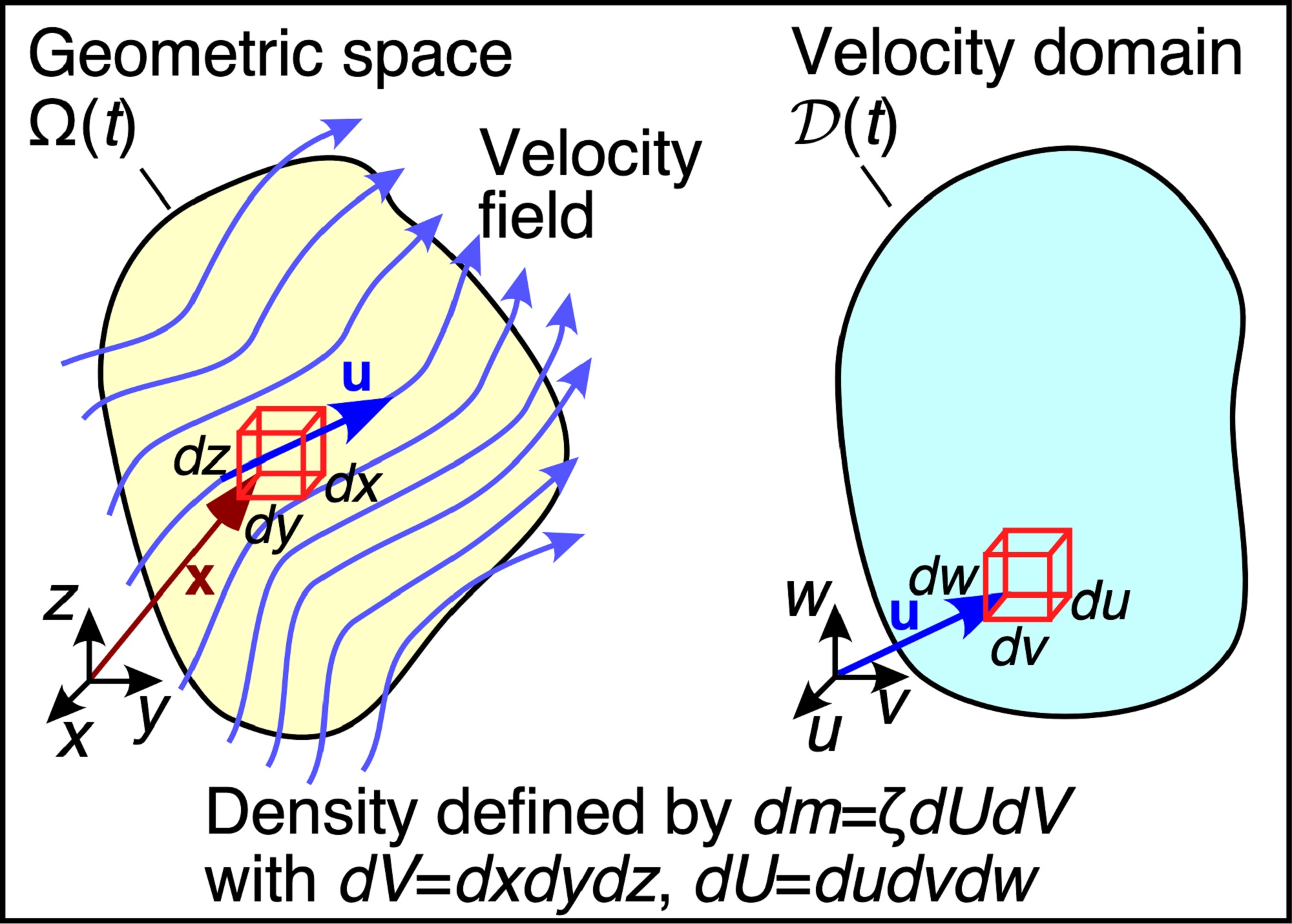
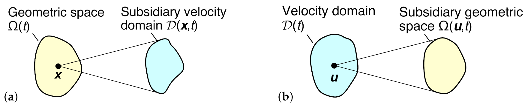
- The geometric representation—the usual physical viewpoint—in which is a function of position and time, and is a function of time. In this perspective, as illustrated in Figure 1a, there exists a map between each position and an entire velocity space , consisting of all possible velocities for this position and time.
- (b)
- The velocimetric representation—an alternative viewpoint—in which is a function of velocity and time, and is a function of time. In this perspective, as illustrated in Figure 1b, there exists a map between each velocity and an entire geometric space , consisting of all possible positions for this velocity and time.
3. A Hierarchy of Densities
3.1. Probability Density Functions
- (a)
- A volumetric pdf [SI units: m−3];
- (b)
- A velocimetric pdf [(m s−1)−3];
- (c)
- A velocivolumetric pdf [m−3 (m s−1)−3];
- (d)
- A conditional velocimetric (ensemble) pdf [(m s−1)−3]; and
- (e)
- A conditional volumetric pdf [m−3];
- (a)
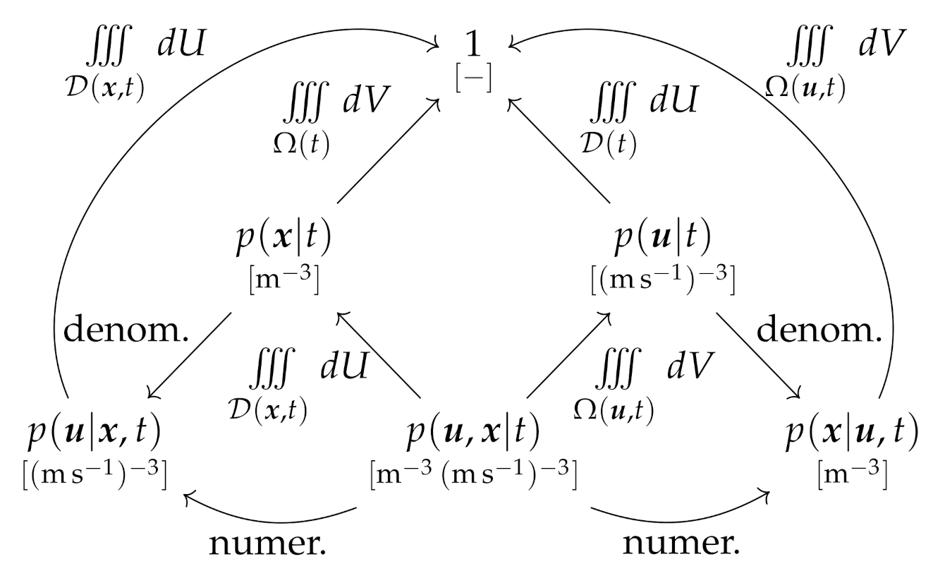
- The velocivolumetric pdf is the most fundamental of the pdfs, giving rise to or by the marginalization operations in Equations (4) and (5), and and by the conditioning operations in Equations (6) and (7). Physically—albeit imprecisely [25,26]—we can interpret as the joint probability of an infinitesimal fluid element having a velocity of and position in , during the time interval .
- (b)
- The volumetric pdf can be recognized as the common probabilistic descriptor for fluid flow systems, forming the basis of the fluid mechanics formulations of the Liouville and Fokker–Planck Equations [27,28,29,30,31], and allied to the volumetric density . Physically, can be interpreted as the probability that a fluid element is situated at the position in the time interval , regardless of velocity.
- (c)
- The velocimetric pdf is rather strange. Physically, can be interpreted as the probability of fluid elements within the control volume having a velocity of in the time interval , regardless of position.
- (d)
- To understand the conditional velocimetric pdf , we interpret as the probability that a fluid element has a velocity of , at the position and time . We therefore recognize —typically but incorrectly written as —as the basis of the ensemble mean commonly used in the Reynolds-averaged Navier–Stokes (RANS) equations, and of the single-position correlation functions of turbulent fluid mechanics [32,33,34,35,36].
- (e)
- To understand the conditional volumetric pdf , we interpret as the probability that a fluid element has a position in , for a velocity of and time .
3.2. Fluid or Material Densities
- (a)
- A volumetric fluid density , [kg m−3];
- (b)
- A velocimetric fluid density Д: , [kg (m s−1)−3];
- (c)
- A velocivolumetric fluid density , [kg m−3 (m s−1)−3];
- (d)
- A conditional velocimetric (ensemble) fluid density , [kg (m s−1)−3]; and
- (e)
- A conditional volumetric fluid density , [kg m−3];
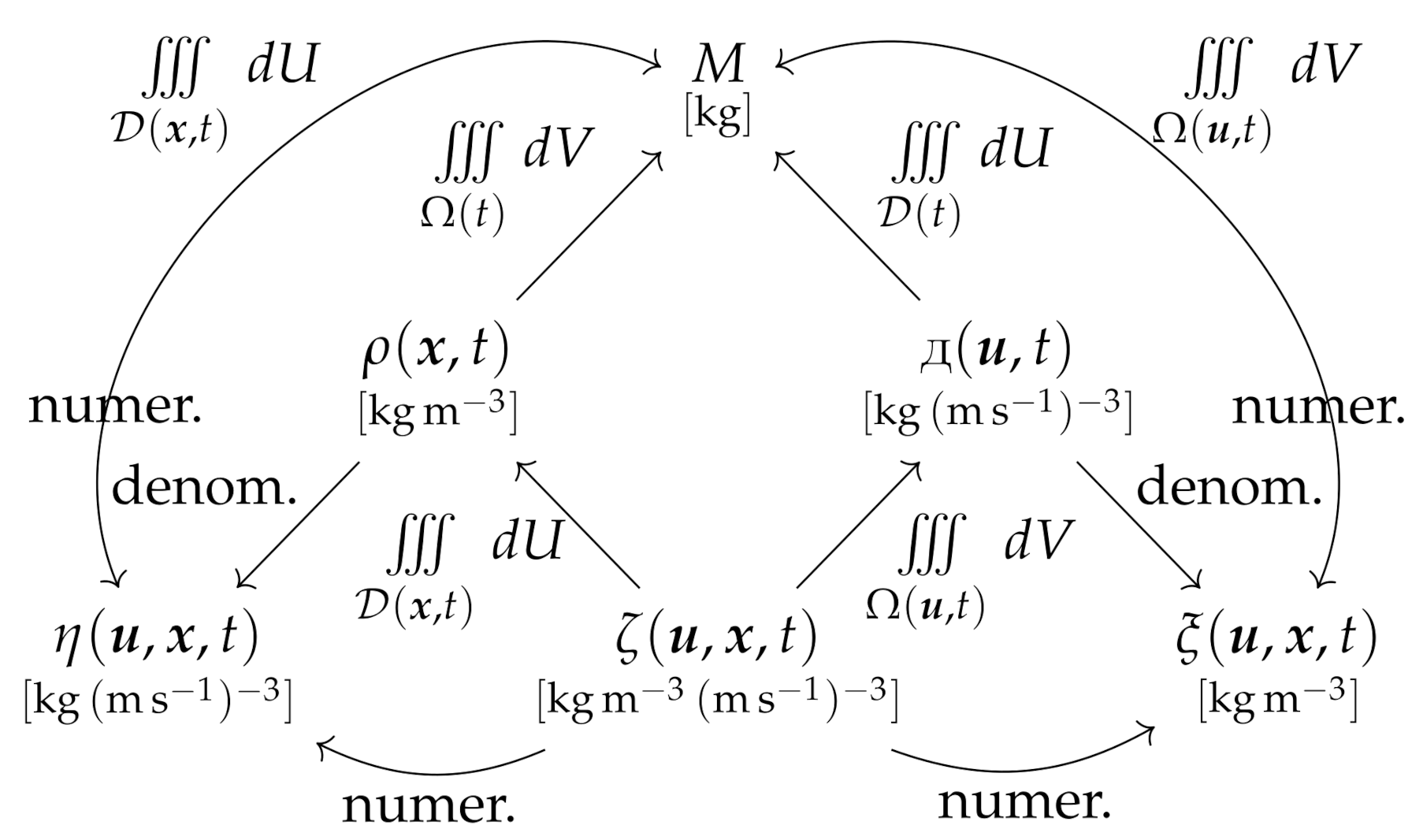
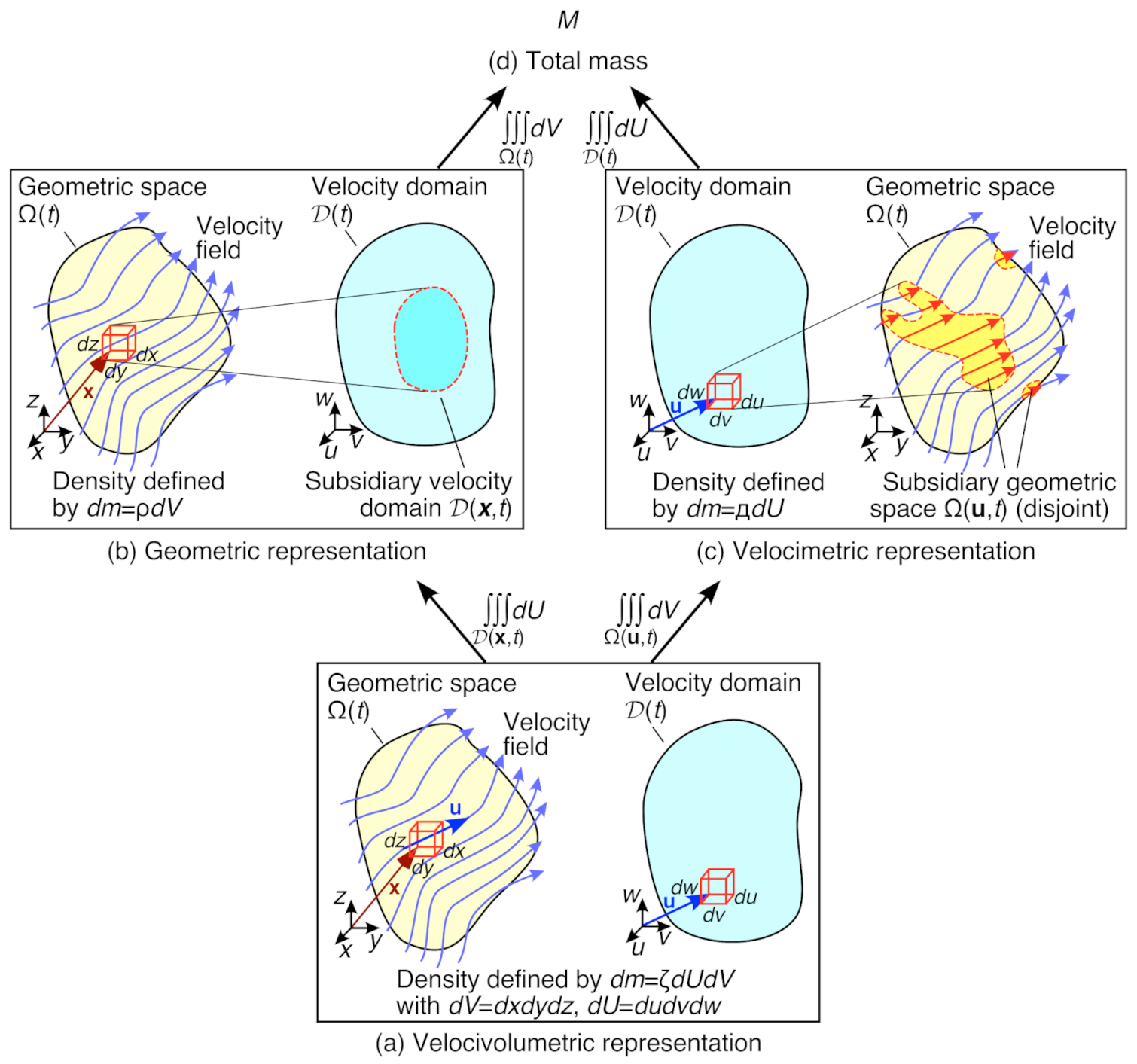
- (a)
- As shown in Figure 4a, the velocivolumetric density represents the fluid mass per unit of velocimetric and geometric space carried by an infinitesimal fluid element of velocity through the infinitesimal control volume element at , during the infinitesimal time interval . In consequence, is both a velocity spectral density and a local volumetric density, accounting for the distribution of fluid mass with both velocity and position. As evident in Figure 3, is central to the current formulation, giving the other fluid densities by marginalization or conditioning.
- (b)
- As shown in Figure 4b, the well-known volumetric fluid density represents the fluid mass per unit volume carried by the fluid through the infinitesimal control volume element at , during the time interval . From Equation (13), is obtained by integration (marginalization) of over the subsidiary velocity domain , consisting of all realizable velocities for this position and time. In well-behaved systems, should consist of an infinitesimal trajectory (or trajectory bundle) in velocity space, from which it may be possible to calculate by line integration.
- (c)
- In contrast, as shown in Figure 4c, the velocimetric density Д represents the fluid mass per unit of velocimetric space transported by fluid elements of velocity throughout the control volume, during the time interval . This is a very strange, aggregated density field, representing the distribution of fluid mass across the velocity spectrum rather than with position, but nonetheless both it and its underlying pdf are well-defined. From Equation (14), Д is obtained by integration (marginalization) of over the subsidiary geometric space , consisting of all realizable positions for this velocity and time. As discussed in Section 2 and illustrated in Figure 4c, in many flow systems will consist of several disjoint but continuous domains, which depending on the flow system may be bounded and may also be closed.
- (d)
- The conditional ensemble density (not illustrated) represents the fluid mass per unit velocimetric space carried by a fluid element of velocity , at the position during the time interval . From Equation (15), is obtained by the ratio of and , which can be interpreted as a conditioning operation over position. This removes the volume from the dimensions of , giving the units of fluid mass per unit velocity space.
- (e)
- The conditional density (not illustrated) represents the fluid mass per unit volume carried by a fluid element in the position , of velocity during the time interval . From Equation (16), is obtained by the ratio of and Д, which can be interpreted as a conditioning operation over velocity. This removes the velocity volume from the dimensions of , giving the units of fluid mass per unit volume.
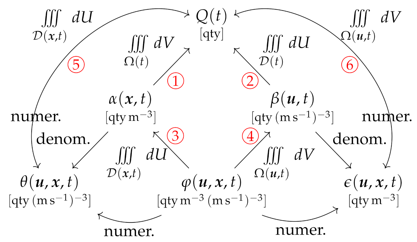
3.3. Generalized Densities
- (a)
- Volumetric densities , [qty m−3];
- (b)
- Velocimetric densities , [qty (m s−1)−3];
- (c)
- Velocivolumetric densities , [qty m−3 (m s−1)−3];
- (d)
- Conditional velocimetric (ensemble) densities , [qty (m s−1)−3]; and
- (e)
- Conditional volumetric densities , [qty m−3];
4. Generalized Formulations of Conservation Equations
4.1. Exterior Calculus Formulations
4.2. Vector Calculus Formulations
5. Example Flow Systems
5.1. Volumetric-Temporal Formulation (Density )
5.2. Velocimetric-Temporal Formulation (Density )
5.3. Velocivolumetric-Temporal Formulation (Density )
5.4. Velocimetric-Temporal Formulation (Density )
5.5. Volumetric-Temporal Formulation (Density )
5.6. Velocimetric-Spatial (Time-Independent) Formulation (Density )
5.7. Volumetric-Velocital (Time-Independent) Formulation (Density )
5.8. Velocimetric-Spatiotemporal Formulation (Density )
5.9. Volumetric-Velocitemporal Formulation (Density )
5.10. Velocimetric-Temporal Formulation (Density )
5.11. Volumetric-Temporal Formulation (Density )
5.12. Discussion
6. Conclusions
Funding
Institutional Review Board Statement
Data Availability Statement
Acknowledgments
Conflicts of Interest
Appendix A. Definition of Densities by Convolution
Appendix B. Philosophical Implications
- 1.
- The frequentist interpretation, in which probabilities are considered to represent measurable frequencies. In this viewpoint, a probability distribution is equivalent to the frequency distribution of an infinite number of random samples collected from a stationary sample space, e.g., [26].
- 2.
- The Bayesian or probabilistic interpretation, in which a probability is a mathematical assignment based on one’s knowledge, which need not correspond to a measurable frequency. Nonetheless, a probability is a rational assignment, which can be calculated and manipulated using the rules of probability theory [82,83].
Appendix C. Extraction of Differential Equations
References
- Reynolds, O. Papers on Mechanical and Physical Subjects; Cambridge University Press: Cambridge, UK, 1903; Volume III. [Google Scholar]
- De Groot, S.R.; Mazur, P. Non-Equilibrium Thermodynamics; Dover Publications: Mineola, NY, USA, 1962. [Google Scholar]
- White, F.M. Fluid Mechanics, 2nd ed.; McGraw-Hill: New York, NY, USA, 1986. [Google Scholar]
- Bird, R.B.; Stewart, W.E.; Lightfoot, E.N. Transport Phenomena, 2nd ed.; John Wiley & Sons: New York, NY, USA, 2006. [Google Scholar]
- Durst, F. Fluid Mechanics, An Introduction to the Theory of Fluid Flows; Springer: Berlin/Heidelberg, Germany, 2008. [Google Scholar]
- Munson, B.R.; Young, D.F.; Okiishi, T.H.; Huebsch, W.W. Fundamentals of Fluid Mechanics, 6th ed.; John Wiley: Hoboken, NJ, USA, 2010. [Google Scholar]
- Dvorkin, E.N.; Goldschmit, M.B. Nonlinear Continua; Springer: Berlin/Heidelberg, Germany, 2006; Chapter 4. [Google Scholar]
- Truesdell, C.; Toupin, R.A. The Classical Field Theories; Flügge, S., Ed.; Handbuch der Physik, Band III/1; Springer: Berlin/Heidelberg, Germany, 1960; p. 347. [Google Scholar]
- Seguin, B.; Hinz, D.F.; Fried, E. Extending the transport theorem to rough domains of integration. Appl. Mech. Rev. 2014, 66, 050802. [Google Scholar] [CrossRef] [PubMed] [Green Version]
- Falach, L.; Segev, R. Reynolds transport theorem for smooth deformations of currents on manifolds. Math. Mech. Solids 2015, 20, 770–786. [Google Scholar] [CrossRef] [Green Version]
- Gurtin, M.E.; Struthers, A.; Williams, W.O. A transport theorem for moving interfaces. Q. Appl. Math. 1989, XLVIII, 773–777. [Google Scholar] [CrossRef] [Green Version]
- Ochoa-Tapia, J.A.; del Rio, J.A.; Whitaker, S. Bulk and surface diffusion in porous media: An application of the surface-averaging theorem. Chem. Eng. Sci. 1993, 48, 2061–2082. [Google Scholar] [CrossRef]
- Slattery, J.C.; Sagis, L.; Oh, E.-S. Interfacial Transport Phenomena, 2nd ed.; Springer: New York, NY, USA, 2007. [Google Scholar]
- Lidström, P. Moving regions in Euclidean space and Reynolds transport theorem. Math. Mech. Solids 2011, 16, 366–380. [Google Scholar] [CrossRef]
- Flanders, H. Differentiation under the integral sign. Am. Math. Mon. 1973, 80, 615–627. [Google Scholar] [CrossRef]
- Marsden, J.E.; Hughes, T.J.R. Mathematical Foundations of Elasticity; Dover Publications: Garden City, NY, USA, 1994. [Google Scholar]
- Lee, J.M. Manifolds and Differential Geometry; American Mathematical Society: Providence, RI, USA, 2009. [Google Scholar]
- Frankel, T. The Geometry of Physics, 3rd ed.; Cambridge University Press: Cambridge, UK, 2013. [Google Scholar]
- Harrison, J. Operator calculus of differential chains and differential forms. J. Geom. Anal. 2015, 25, 357–420. [Google Scholar] [CrossRef] [Green Version]
- Tai, C.-T. Generalized Vector and Dyadic Analysis; IEEE: New York, NY, USA, 1992. [Google Scholar]
- Mémin, E. Fluid flow dynamics under location uncertainty. Geophys. Astrophys. Fluid Dyn. 2014, 108, 119–146. [Google Scholar] [CrossRef] [Green Version]
- Crisan, D.; Holm, D.D.; Leahy, J.-M.; Nilssen, T. Variational principles for fluid dynamics on rough paths. arXiv 2020, arXiv:2004.07829v1. [Google Scholar] [CrossRef]
- Niven, R.K.; Cordier, L.; Kaiser, E.; Schlegel, M.; Noack, B.R. Rethinking the Reynolds transport theorem, Liouville equation, and Perron-Frobenius and Koopman operators. arXiv 2020, arXiv:1810.06022v5. [Google Scholar]
- Niven, R.K.; Cordier, L.; Kaiser, E.; Schlegel, M.; Noack, B.R. New conservation laws based on generalised Reynolds transport theorems, paper 110. In Proceedings of the 22nd Australasian Fluid Mechanics Conference (AFMC2020), Brisbane, Australia, 7–10 December 2020; Chanson, H., Brown, R., Eds.; University of Queensland: Brisbane, Australia, 2021. [Google Scholar]
- Hoel, P.G. Introduction to Mathematical Statistics, 3rd ed.; John Wiley: New York, NY, USA, 1962. [Google Scholar]
- Feller, W. An Introduction to Probability Theory and Its Applications; John Wiley and Sons, Inc.: New York, NY, USA, 1966; Volume II. [Google Scholar]
- Liouville, J. Note sur la théorie de la variation des constantes arbitraires. J. MathÉmatiques Pures AppliquÉes 1838, 1, 342–349. (In French) [Google Scholar]
- Risken, H. The Fokker–Planck Equation: Methods of Solution and Applications; Springer: Berlin/Heidelberg, Germany, 1984. [Google Scholar]
- Lützen, J. Joseph Liouville 1809–1882. Master of Pure and Applied Mathematics; Springer: New York, NY, USA, 1990; pp. 637–708. [Google Scholar]
- Ehrendorfer, M. The Liouville equation in atmospheric predictability, Seminar on Predictability of Weather and Climate. In Proceedings of the European Centre for Medium-Range Weather Forecasts (ECMWF), Reading, UK, 9–13 September 2002; pp. 47–81. [Google Scholar]
- Pottier, N. Nonequilibrium Statistical Physics: Linear Irreversible Processes; Oxford University Press: Oxford, UK, 2010. [Google Scholar]
- Batchelor, G.K. Theory of Homogeneous Turbulence; Cambridge University Press: Cambridge, UK, 1967. [Google Scholar]
- Monin, A.S.; Yaglom, A.M. Statistical Fluid Mechanics: Mechanics of Turbulence; Dover Publications: Garden City, NY, USA, 1971; Volume I. [Google Scholar]
- Hinze, J.O. Turbulence: An Introduction to its Mechanism and Theory, 2nd ed.; McGraw-Hill: New York, NY, USA, 1975. [Google Scholar]
- Pope, S.B. Turbulent Flows; Cambridge University Press: Cambridge, UK, 2000. [Google Scholar]
- Davidson, P.A. Turbulence: An Introduction for Scientists and Engineers; Oxford University Press: Oxford, UK, 2004. [Google Scholar]
- Burlington, R.S.; May, D.C. Handbook of Probability and Statistics with Tables; Handbook Publisher: Sandusky, OH, USA, 1958. [Google Scholar]
- Jaynes, E.T. The minimum entropy production principle. Ann. Rev. Phys. Chem. 1980, 31, 579–601. [Google Scholar] [CrossRef]
- González, D.; Davis, S.; Gutiérrez, G. Newtonian dynamics from the principle of maximum caliber. arXiv 2013, arXiv:1310.1382v1. [Google Scholar] [CrossRef] [Green Version]
- Ghosh, K.; Dixit, P.D.; Agozzino, L.; Dill, K.A. The maximum caliber variational principle for nonequilibria. Annu. Rev. Phys. Chem. 2020, 71, 213–238. [Google Scholar] [CrossRef] [Green Version]
- Matheron, G. Les Variables Régionalisées et Leur Estimation, Une Application de la Théorie de Fonctions Aléatoires Aux Sciences de la Nature; Masson et Cie: Paris, France, 1965. [Google Scholar]
- Marle, C.M. Écoulements monophasiques en milieu poreux. Rev. Inst. Français Pétrole 1967, 22, 1471–1509. [Google Scholar]
- Anderson, T.B.; Jackson, R. A fluid mechanical description of fluidized beds. Ind. Engng Chem. Fundam. 1967, 6, 527–539. [Google Scholar] [CrossRef]
- Whitaker, S. Diffusion and dispersion in porous media. AIChE J. 1967, 13, 420–427. [Google Scholar] [CrossRef]
- Whitaker, S. Advances in theory of fluid motion in porous media. Ind. Eng. Chem. 1969, 61, 14–28. [Google Scholar] [CrossRef]
- Bachmat, Y. Spatial macroscopization of processes in heterogeneous systems. Isr. J. Technol. 1972, 10, 391–403. [Google Scholar]
- Gray, W.G.; Lee, P.C.Y. On the theorems for local volume averaging of multiphase systems. Int. J. Multiphase Flow 1977, 3, 333–340. [Google Scholar] [CrossRef]
- Hassanizadeh, M.; Gray, W.G. General conservation equations for multi-phase systems: 1. Averaging procedure. Adv. Water Resour. 1979, 2, 131–144, and Errata 3, 91–94. [Google Scholar] [CrossRef]
- Narasimhan, T.N. A note on volume-averaging. Adv. Water Res. 1980, 3, 135–139. [Google Scholar] [CrossRef]
- Ene, H.L. On the thermodynamic theory of mixtures. Int. J. Eng. Sci. 1981, 19, 905–914. [Google Scholar] [CrossRef]
- Cushman, J.H. Proofs of the volume averaging theorems for multiphase flow. Adv Water Resour. 1982, 5, 248–253. [Google Scholar] [CrossRef]
- Cushman, J.H. Volume averaging, probabilistic averaging, and ergodicity. Adv. Water Resour. 1983, 6, 182–184. [Google Scholar] [CrossRef]
- Baveye, P.; Sposito, G. The operational significance of the continuum hypothesis in the theory of water movement through soils and aquifers. Water Resour. Res. 1984, 20, 521–530. [Google Scholar] [CrossRef]
- Cushman, J.H. On unifying the concepts of scale, instrumentation, and stochastics in the development of multiphase transport theory. Water Res. Res. 1984, 20, 1668–1676. [Google Scholar]
- Cushman, J.H. Multiphase transport based on compact distributions. Acta Appl. Math. 1985, 3, 239–254. [Google Scholar] [CrossRef]
- Bear, J.; Bachmat, Y. Introduction to Modeling of Transport Phenomena in Porous Media; Kluwer Academic Publishers: Dordrecht, The Netherlands, 1991. [Google Scholar]
- Gray, W.G.; Leijnse, A.; Kolar, R.L.; Blain, C.A. Mathematical Tools for Changing Scale in the Analysis of Physical Systems; CRC Press: Roca Raton, FL, USA, 1993. [Google Scholar]
- Quintard, M.; Whitaker, S. Transport in ordered and disordered porous media: Volume-averaged equations, closure problems, and comparison with experiment. Chem. Eng. Sci. 1993, 48, 2537–2564. [Google Scholar] [CrossRef]
- Chen, Z. Large-scale averaging analysis of single phase flow in fractured reservoirs. SIAM J. Appl. Math. 1994, 54, 641–659. [Google Scholar]
- Grau, R.J.; Cantero, H.J. A systematic time-, space- and time-space-averaging procedure for bulk phase equations in systems with multiphase flow. Chem. Eng. Sci. 1994, 49, 449–461. [Google Scholar] [CrossRef]
- Cushman, J.H. The Physics of Fluids in Hierarchical Porous Media: Angstroms to Miles; Springer: New York, NY, USA, 1997. [Google Scholar]
- Whitaker, S. The Method of Volume Averaging; Kluwer Academic Publishers: Dordrecht, The Netherlands, 1999. [Google Scholar]
- Gray, W.G.; Miller, C.T. Thermodynamically constrained averaging theory approach for modeling flow and transport phenomena in porous medium systems: 2. Foundation. Adv. Water Resour. 2005, 28, 181–202. [Google Scholar] [CrossRef]
- Wood, W.D. Technical note: Revisiting the geometric theorems for volume averaging. Adv. Water Resour. 2013, 62, 340–352. [Google Scholar] [CrossRef]
- Gray, W.G.; Miller, C.T. A generalization of averaging theorems for porous medium analysis. Adv. Water Resour. 2013, 62, 227–237. [Google Scholar] [CrossRef]
- Pokrajac, P.; de Lemos, M.J.S. Spatial averaging over a variable volume and Its application to boundary-layer flows over permeable walls. J. Hydraul. Eng. 2015, 141, 04014087. [Google Scholar] [CrossRef]
- Davit, Y.; Quintard, M. Technical notes on volume averaging in porous media I: How to choose a spatial averaging operator for periodic and quasiperiodic structures. Transp Porous Med. 2017, 119, 555–584. [Google Scholar] [CrossRef]
- Takatsu, Y. Modification of the fundamental theorem for transport phenomena in porous media. Int. J. Heat and Mass Transfer 2017, 115, 1109–1120. [Google Scholar] [CrossRef]
- Kobayashi, S.; Nomizu, K. Foundations of Differential Geometry; John Wiley & Sons: New York, NY, USA; Interscience Publishers: New York, NY, USA, 1963; Volume 1. [Google Scholar]
- Guggenheimer, H.W. Differential Geometry; McGraw-Hill: New York, NY, USA, 1963; Dover Publications: Garden City, NY, USA, 1977. [Google Scholar]
- Cartan, H. Differential Forms; Dover Publications: Garden City, NY, USA, 1970. [Google Scholar]
- Lovelock, D.; Rund, H. Tensors, Differential Forms, and Variational Principles; Dover Publications: Garden City, NY, USA, 1989. [Google Scholar]
- Olver, P.J. Applications of Lie Groups to Differential Equations, 2nd ed.; Springer: New York, NY, USA, 1993. [Google Scholar]
- Torres del Castillo, G. Differentiable Manifolds; Springer: New York, NY, USA, 2012. [Google Scholar]
- Bachman, D. A Geometric Approach to Differential Forms, 2nd ed.; Birkhäuser: Boston, MA, USA, 2012. [Google Scholar]
- Sjamaar, R. Manifolds and Differential Forms; Cornell University: Ithaca, NY, USA, 2017. [Google Scholar]
- Hutter, K.; Jöhnk, K.D. Continuum Methods of Physical Modeling; Springer: New York, NY, USA, 2004. [Google Scholar]
- Spurk, J.H. Fluid Mechanics; Springer: Berlin/Heidelberg, Germany, 1997. [Google Scholar]
- Weinstock, R. Calculus of Variations; Dover Publications: Mineola, NY, USA, 1974. [Google Scholar]
- Truesdell, C. The Kinematics of Vorticity; Dover Publications: Mineola, NY, USA, 2018. [Google Scholar]
- Reddiger, M.; Poirier, B. The differentiation lemma and the Reynolds transport theorem for submanifolds with corners. arXiv 2021, arXiv:1906.03330v5. [Google Scholar]
- Cox, R.T. The Algebra of Probable Inference; John Hopkins Press: Baltimore, MD, USA, 1961. [Google Scholar]
- Jaynes, E.T. Probability Theory: The Logic of Science; Bretthorst, G.L., Ed.; Cambridge University Press: Cambridge, UK, 2003. [Google Scholar]


| Symbol | Description | SI Units | |
|---|---|---|---|
| Mathematical Operators | |||
| transpose | |||
| · | vector scalar product | ||
| × | cross product; multiplication symbol (only if there is a line break in the equation) | ||
| ∂ | partial derivative operator; boundary of domain | ||
| vector partial derivative operator with respect to | |||
| gradient operator with respect to | |||
| velocital gradient operator with respect to | (m s−1)−1 | ||
| spatial gradient operator with respect to | m−1 | ||
| gradient operator with respect to | |||
| velocitotemporal gradient operator with respect to | [(m s−1), (m s), (m s), s] | ||
| spatiotemporal gradient operator with respect to | [m, m, m, s] | ||
| expectation over small volume | |||
| expectation over small velocity domain | |||
| integral over volume | |||
| integral over velocity domain | |||
| ∧ | wedge product | ||
| ∟ | augmentation operator, such that is the tensor based on coordinates augmented by parameter | ||
| ➀ | integral path as labeled in Figure 5 | ||
| Conventions | |||
| Vector derivatives are defined by the convention | |||
| The product of two vectors implies a tensor, e.g., | |||
| The divergence of a tensor is rotated, e.g., | |||
| Roman symbols | |||
| c | index of chemical species; index of components of | ||
| cth component of | |||
| generalized m-dimensional parameter vector | |||
| control volume = reference frame for fluid motion | |||
| d | differential of a function; exterior derivative of a differential form | ||
| extended exterior derivative based on augmented coordinates | |||
| total derivative in time | s | ||
| infinitesimal area element in volumetric space | m2 | ||
| directed infinitesimal area element in volumetric space | m2 | ||
| infinitesimal surface element in velocimetric space | (m s)2 | ||
| directed infinitesimal surface element in velocimetric space | (m s)2 | ||
| infinitesimal element of fluid mass | kg | ||
| infinitesimal element of velocimetric space | (m s)3 | ||
| infinitesimal element of volumetric space | m3 | ||
| cotangent to jth component of generalized vector | |||
| generalized directed area element on | |||
| generalized volume element in | |||
| vector of spatiotemporal SI units | [m, m, m, s] | ||
| vector of velocitotemporal SI units | [m s, m s, m s, s] | ||
| substantial or material derivative in time | s | ||
| velocimetric domain | |||
| local specific total energy | J kg | ||
| velocity-distinct specific energy | J kg | ||
| velocity-distinct local specific energy | J kg | ||
| E | total energy | J | |
| sum of forces | N | ||
| acceleration due to gravity | m s | ||
| velocity gradient tensor field | (m s) m = s | ||
| augmented velocity gradient tensor field | [s, s, s, m s] | ||
| electrical flux | C m s = A m | ||
| multivariate interior product with respect to over parameters | |||
| I | net inward electrical current (passive sign convention) | C s = A | |
| identity matrix of size m | |||
| j | index of components of generalized coordinates | ||
| molar flux of species c | mol m s | ||
| heat flux | J m s | ||
| entropy flux | J K m s | ||
| multivariate Lie derivative with respect to over parameters | |||
| multivariate Lie derivative with respect to over parameters | |||
| LHS | left-hand side | ||
| small fluid mass domain | |||
| m | dimension of vector parameter | ||
| orientable differentiable manifold; generalized space | |||
| M | total fluid mass | kg | |
| rate of change of total fluid mass | kg s | ||
| rate of change of mass of species c | kgc s | ||
| molar mass of species c | kgc mol | ||
| n | dimension of manifold M, dimension of coordinates | ||
| outward unit normal to in volumetric space | |||
| outward unit normal to in velocimetric space | |||
| conditional pdf of a and b subject to c | units of | ||
| P | pressure | Pa = J m | |
| Q | total conserved quantity (of any type) | qty | |
| net inward heat flow rate | J s | ||
| r | dimension of submanifold , dimension of differential form | ||
| local Cartesian position coordinates | m | ||
| local radius of a lever arm | m | ||
| velocity-distinct radius of a lever arm | m | ||
| velocity-distinct local radius of a lever arm | m | ||
| RHS | right-hand side | ||
| local specific entropy | J K kg | ||
| velocity-distinct specific entropy | J K kg | ||
| velocity-distinct local specific entropy | J K kg | ||
| local Cartesian velocity coordinates | m s | ||
| S | total entropy | J K | |
| total net inward non-fluid entropy flow rate | J K s | ||
| t | time | s | |
| sum of torques | N m | ||
| Cartesian velocity field | m s | ||
| Cartesian local acceleration field | m s | ||
| small velocity domain | |||
| volume of an infinitesimal n-dimensional parallelopiped spanned by the cotangents to | |||
| th component of generalized vector or tensor field | |||
| generalized vector or tensor field | |||
| small fluid volume | |||
| net inward work flow rate | J s | ||
| Cartesian position coordinates | m | ||
| Cartesian Lagrangian position coordinates | m | ||
| jth component of vector | |||
| generalized n-dimensional local or global Cartesian coordinates | |||
| charge per mass of species c | C kgc | ||
| local specific charge | C kg | ||
| velocity-distinct specific charge | C kg | ||
| velocity-distinct local specific charge | C kg | ||
| Z | total charge | C | |
| Greek symbols | |||
| generalized volumetric density | qty m | ||
| local generalized specific density | qty kg | ||
| generalized velocimetric density | qty (m s) | ||
| velocity-distinct generalized specific density | qty kg | ||
| inverse velocity gradient tensor field | m (m s) = s | ||
| augmented inverse velocity gradient tensor field, | [s, s, s, m s] | ||
| Kronecker delta tensor | |||
| generalized conditional volumetric density | qty m | ||
| velocity-distinct local generalized specific density | qty kg | ||
| velocivolumetric fluid mass density | kg m (m s) | ||
| velocivolumetric mass density of species c | kgc m (m s) | ||
| conditional velocimetric fluid mass density | kg (m s) | ||
| conditional velocimetric mass density of species c | kgc (m s) | ||
| generalized conditional velocimetric density | qty (m s) | ||
| velocity-distinct local generalized specific density | qty kg | ||
| conditional volumetric fluid mass density | kg m | ||
| conditional volumetric mass density of species c | kgc m | ||
| molar rate of production of species c | mol m s | ||
| volumetric fluid mass density | kg m | ||
| volumetric mass density of species c | kgc m | ||
| total entropy production | J K s | ||
| local entropy production | J K m s | ||
| stress tensor (positive in compression) | Pa = J m | ||
| multivariate flow generated by | |||
| augmented multivariate flow generated by | |||
| generalized velocivolumetric density | qty m (m s) | ||
| velocity-distinct local generalized specific density | qty kg | ||
| local specific mass density of species c | kgc kg | ||
| velocity-distinct specific mass density of species c | kgc kg | ||
| velocity-distinct local specific mass density of species c | kgc kg | ||
| generalized density of conserved quantity in generalized space | |||
| r-form, n-form (respectively) in submanifold | |||
| general submanifold or domain; volumetric domain (fluid volume or material volume) | |||
| Cyrillic symbols | |||
| Д | velocimetric fluid mass density | kg (m s) | |
| velocimetric mass density of species c | kgc (m s) | ||
| Conserved Quantity | Density | Integral Equation | Differential Equation | ||||
|---|---|---|---|---|---|---|---|
| LHS = = | = RHS | SI Units | LHS | = RHS | SI Units | ||
| Fluid mass | [kg s] | 0 | [kg s m] | ||||
| Species mass | [kgc s] | [kgc s m] | |||||
| Linear momentum | [(kg m s) s = N] | [N m] | |||||
| Angular momentum | [(kg m s) s = N m] | [N m = (N m) m] | |||||
| Energy | [J s = W] | [J s m = W m] | |||||
| Charge (in solution) | [C s = A] | [C s m = A m] | |||||
| Entropy | [J K s] | [J K s m] | |||||
| Probability | [s] | 0 | [s m] | ||||
| Conserved Quantity | Density | Integral Equation | Differential Equation | ||||
|---|---|---|---|---|---|---|---|
| LHS = = | = RHS | SI Units | LHS | = RHS | SI Units | ||
| Fluid mass | Д | [kg s] | 0 | [kg s (m s)] | |||
| Species mass | [kgc s] | [kgc s (m s)] | |||||
| Linear momentum | [(kg m s) s = N] | [N (m s)] | |||||
| Angular momentum | [(kg m s) s = N m] | [(N m) (m s)] | |||||
| Energy | [J s = W] | [J s (m s) = W (m s)] | |||||
| Charge (in solution) | [C s = A] | [C s (m s) = A (m s)] | |||||
| Entropy | [J K s] | [J K s (m s)] | |||||
| Probability | [s] | 0 | [s (m s)] | ||||
| Conserved Quantity | Density | Integral Equation | Differential Equation | ||||
|---|---|---|---|---|---|---|---|
| LHS = = | = RHS | SI Units | LHS | = RHS | SI Units | ||
| Fluid mass | [kg s] | 0 | [kg s m (m s)] | ||||
| Species mass | = | [kgc s] | [kgc s m (m s)] | ||||
| Linear momentum | [(kg m s) s = N] | [N m (m s)] | |||||
| Angular momentum | [(kg m s) s = N m] | [(N m) m (m s)] | |||||
| Energy | [J s = W] | [J s m (m s)] | |||||
| Charge (in solution) | [C s = A] | [C s m (m s)] | |||||
| Entropy | [J K s] | [J K s m (m s)] | |||||
| Probability | [s] | 0 | [s m (m s)] | ||||
| Conserved Quantity | Density | Integral Equation | Differential Equation | ||||
|---|---|---|---|---|---|---|---|
| LHS = | = RHS | SI Units | LHS | = RHS | SI Units | ||
| Fluid mass | [kg m s] | [kg m s] | |||||
| Species mass | = | [kgc m s] | [kgc m s] | ||||
| Linear momentum | [(kg m s) m s = N m] | [N m] | |||||
| Angular momentum | [(kg m s) m s = (N m) m] | [(N m) m] | |||||
| Energy | [J m s = W m] | [J m s = W m] | |||||
| Charge (in solution) | [C m s = A m] | [C m s = A m] | |||||
| Entropy | [J K m s] | [J K m s] | |||||
| Probability | [m s] | [m s] | |||||
| [s] | 0 | [(m s) s] | |||||
| Conserved Quantity | Density | Integral Equation | Differential Equation | ||||
|---|---|---|---|---|---|---|---|
| LHS = | = RHS | SI Units | LHS | = RHS | SI Units | ||
| Fluid mass | [kg (m s) s] | [kg (m s) s] | |||||
| Species mass | = | [kgc (m s) s] | [kgc (m s) s] | ||||
| Linear momentum | [(kg m s) (m s) s = N (m s)] | [N (m s)] | |||||
| Angular momentum | [(kg m s) (m s) s = (N m) (m s)] | [(N m) (m s)] | |||||
| Energy | [J (m s) s = W (m s)] | [J (m s) s = W (m s)] | |||||
| Charge (in solution) | [C (m s) s = A (m s)] | [C (m s) s = A (m s)] | |||||
| Entropy | [J K (m s) s] | [J K (m s) s] | |||||
| Probability | [(m s) s] | [(m s) s] | |||||
| [s] | 0 | [m s] | |||||
| Conserved Quantity | Density | Integral Equation | Differential Equation | ||||
|---|---|---|---|---|---|---|---|
| LHS = | = RHS | SI Units | LHS | = RHS | SI Units | ||
| Fluid mass | [kg m−4 = kg m m] | [kg m−4 = kg m m] | |||||
| Species mass | [kgc m−4 = kgc m m] | [kgc m−4 = kgc m m] | |||||
| Linear momentum | [kg m s = (kg m s) m m] | [kg m s] | |||||
| Angular momentum | [kg m s = (kg m2 s) m m] | [kg m s] | |||||
| Energy | [J m m] | [J m m] | |||||
| Charge (in solution) | [C m m] | [C m m] | |||||
| Entropy | [J K m m] | [J K m m] | |||||
| Probability | [m m] | [m m] | |||||
| [m] | [(m s) m] | ||||||
| Conserved Quantity | Density | Integral Equation | Differential Equation | ||||
|---|---|---|---|---|---|---|---|
| LHS = | = RHS | SI Units | LHS | = RHS | SI Units | ||
| Fluid mass | [kg (m s)−4 = kg (m s) (m s)] | [kg (m s)−4 = kg (m s) (m s)] | |||||
| Species mass | [kgc (m s)−4 = kgc (m s) (m s)] | [kgc (m s)−4 = kgc (m s) (m s)] | |||||
| Linear momentum | [kg (m s) = (kg m s) (m s) (m s)] | [kg (m s)] | |||||
| Angular momentum | [kg m (m s) = (kg m2 s) (m s) (m s)] | [kg m (m s)] | |||||
| Energy | [J (m s) (m s)] | [J (m s) (m s)] | |||||
| Charge (in solution) | [C (m s) (m s)] | [C (m s) (m s)] | |||||
| Entropy | [J K (m s) (m s)] | [J K (m s) (m s)] | |||||
| Probability | [(m s) (m s)] | [(m s) (m s)] | |||||
| [(m s)] | [m (m s)] | ||||||
| Conserved Quantity | Density | Integral Equation | Differential Equation | ||||
|---|---|---|---|---|---|---|---|
| LHS = | = RHS | SI Units | LHS | = RHS | SI Units | ||
| Fluid mass | [kg m ] | [kg m ] | |||||
| Species mass | [kgc m ] | [kgc m ] | |||||
| Linear momentum | [(kg m s) m ] | [(kg m s) m ] | |||||
| Angular momentum | [(kg m2 s) m ] | [(kg m2 s) m ] | |||||
| Energy | [J m ] | [J m ] | |||||
| Charge (in solution) | [C m ] | [C m ] | |||||
| Entropy | [J K m ] | [J K m ] | |||||
| Probability | [m ] | [m ] | |||||
| [] | [(m s) ] | ||||||
| Conserved quantity | Density | Integral Equation | Differential Equation | ||||
|---|---|---|---|---|---|---|---|
| LHS = | = RHS | SI Units | LHS | = RHS | SI Units | ||
| Fluid mass | [kg (m s) ] | [kg (m s) ] | |||||
| Species mass | [kgc (m s) ] | [kgc (m s) ] | |||||
| Linear momentum | [(kg m s) (m s) ] | [(kg m s) (m s) ] | |||||
| Angular momentum | [(kg m2 s) (m s) ] | [(kg m2 s) (m s) ] | |||||
| Energy | [J (m s) ] | [J (m s) ] | |||||
| Charge (in solution) | [C (m s) ] | [C (m s) ] | |||||
| Entropy | [J K (m s) ] | [J K (m s)] | |||||
| Probability | [(m s) ] | [(m s) ] | |||||
| [] | [m ] | ||||||
| Conserved Quantity | Density | Integral Equation | Differential Equation | ||||
|---|---|---|---|---|---|---|---|
| LHS = = | = RHS | SI Units | LHS | = RHS | SI Units | ||
| Fluid mass | [kg s] | 0 | [kg s (m s)] | ||||
| Species mass | = | [kgc s] | [kgc s (m s)] | ||||
| Linear momentum | [(kg m s) s = N] | [N (m s)] | |||||
| Angular momentum | [(kg m s) s = N m] | [(N m) (m s)] | |||||
| Energy | [J s = W] | [J s (m s) = W (m s)] | |||||
| Charge (in solution) | [C s = A] | [C s (m s) = A (m s)] | |||||
| Entropy | [J K s] | [J K s (m s)] | |||||
| Probability | [s] | 0 | [(m s) s] | ||||
| Conserved quantity | Density | Integral Equation | Differential Equation | ||||
|---|---|---|---|---|---|---|---|
| LHS = = | = RHS | SI Units | LHS | = RHS | SI Units | ||
| Fluid mass | [kg s] | 0 | [kg s m] | ||||
| Species mass | [kgc s] | [kgc s m] | |||||
| Linear momentum | [(kg m s) s = N] | [N m] | |||||
| Angular momentum | [(kg m s) s = N m] | [N m = (N m) m] | |||||
| Energy | [J s = W] | [J s m = W m] | |||||
| Charge (in solution) | [C s = A] | [C s m = A m] | |||||
| Entropy | [J K s] | [J K s m] | |||||
| Probability | [s] | 0 | [s m] | ||||
Publisher’s Note: MDPI stays neutral with regard to jurisdictional claims in published maps and institutional affiliations. |
© 2022 by the author. Licensee MDPI, Basel, Switzerland. This article is an open access article distributed under the terms and conditions of the Creative Commons Attribution (CC BY) license (https://creativecommons.org/licenses/by/4.0/).
Share and Cite
Niven, R.K. A Hierarchy of Probability, Fluid and Generalized Densities for the Eulerian Velocivolumetric Description of Fluid Flow, for New Families of Conservation Laws. Entropy 2022, 24, 1493. https://doi.org/10.3390/e24101493
Niven RK. A Hierarchy of Probability, Fluid and Generalized Densities for the Eulerian Velocivolumetric Description of Fluid Flow, for New Families of Conservation Laws. Entropy. 2022; 24(10):1493. https://doi.org/10.3390/e24101493
Chicago/Turabian StyleNiven, Robert K. 2022. "A Hierarchy of Probability, Fluid and Generalized Densities for the Eulerian Velocivolumetric Description of Fluid Flow, for New Families of Conservation Laws" Entropy 24, no. 10: 1493. https://doi.org/10.3390/e24101493