
Analyzing Transverse Momentum Spectra of Pions, Kaons and Protons in p–p, p–A and A–A Collisions via the Blast-Wave Model with Fluctuations


Abstract
:1. Introduction
2. Formalism and Method
3. Results and Discussion
4. Summary and Conclusions
Author Contributions
Funding
Institutional Review Board Statement
Informed Consent Statement
Data Availability Statement
Conflicts of Interest
References
- Ivanenko, D.D.; Kurdgelaidze, D.F. Hypothesis concerning quark stars. Astrophysics 1965, 1, 251–252. [Google Scholar] [CrossRef]
- Itoh, N. Hydrostatic equilibrium of hypothetical quark stars. Prog. Theor. Phys. 1970, 44, 291. [Google Scholar] [CrossRef] [Green Version]
- Lee, T.D.; Wick, G.C. Vacuum stability and vacuum excitation in a spin-0 field theory. Phys. Rev. D 1974, 9, 2291–2316. [Google Scholar] [CrossRef] [Green Version]
- Uphoff, J.; Fochler, O.; Xu, Z.; Greiner, C. RHIC and LHC phenomena with a unified parton transport. Acta Phys. Pol. B Proc. Supp. 2012, 5, 555. [Google Scholar] [CrossRef]
- Zhong, Y.; Yang, C.B.; Cai, X.; Feng, S.Q. A systematic study of magnetic field in Relativistic Heavy-ion Collisions in the RHIC and LHC energy regions. Adv. High Energy Phys. 2014, 2014, 193039. [Google Scholar] [CrossRef] [Green Version]
- Chatterjee, S.; Das, S.; Kumar, L.; Mishra, D.; Mohanty, B.; Sahoo, R.; Sharma, N. Freeze-out parameters in heavy-ion collisions at AGS, SPS, RHIC, and LHC energies. Adv. High Energy Phys. 2015, 2015, 349013. [Google Scholar] [CrossRef]
- Hwa, R.C. Recognizing critical behavior amidst minijets at the Large Hadron Collider. Adv. High Energy Phys. 2015, 2015, 526908. [Google Scholar] [CrossRef] [Green Version]
- Ma, G.L.; Nie, M.W. Properties of full jet in High-Energy Heavy-Ion Collisions from parton scatterings. Adv. High Energy Phys. 2015, 2015, 967474. [Google Scholar] [CrossRef]
- Adamczyk, L.; Adkins, J.K.; Agakishiev, G.; Aggarwal, M.M.; Ahammed, Z.; Alekseev, I.; Alford, J.; Aparin, A.; Arkhipkin, D.; Aschenauer, E.C.; et al. Measurements of dielectron production in Au + Au collisions at GeV from the STAR experiment. Phys. Rev. C 2015, 92, 024912. [Google Scholar] [CrossRef] [Green Version]
- Xu, N. for the STAR Collaboration. An overview of STAR experimental results. Nucl. Phys. A 2014, 931, 1–12. [Google Scholar] [CrossRef] [Green Version]
- Chatterjee, S.; Mohanty, B.; Singh, R. Freezeout hypersurface at energies available at the CERN Large Hadron Collider from particle spectra: Flavor and centrality dependence. Phys. Rev. C 2015, 92, 024917. [Google Scholar] [CrossRef]
- Chatterjee, S.; Mohanty, B. Production of light nuclei in heavy-ion collisions within a multiple-freezeout scenario. Phys. Rev. C 2014, 90, 034908. [Google Scholar] [CrossRef] [Green Version]
- Räsänen, S.S. For the ALICE Collaboration. ALICE overview. EPJ Web Conf. 2016, 126, 02026. [Google Scholar] [CrossRef] [Green Version]
- Floris, M. Hadron yields and the phase diagram of strongly interacting matter. Nucl. Phys. A 2014, 931, 103. [Google Scholar] [CrossRef] [Green Version]
- Das, S.; Mishra, D.; Chatterjee, S.; Mohanty, B. Freeze-out conditions in proton-proton collisions at the highest energies available at the BNL Relativistic Heavy Ion Collider and the CERN Large Hadron Collider. Phys. Rev. C 2017, 95, 014912. [Google Scholar] [CrossRef] [Green Version]
- Huovinen, P. Chemical freeze-out temperature in the hydrodynamical description of Au+Au collisions at GeV. Eur. Phys. J. A 2008, 37, 121. [Google Scholar] [CrossRef] [Green Version]
- De, B. Non-extensive statistics and understanding particle production and kinetic freeze-out process from pT-spectra at 2.76 TeV. Eur. Phys. J. A 2014, 50, 138. [Google Scholar] [CrossRef] [Green Version]
- Andronic, A. An overview of the experimental study of quark-gluon matter in high-energy nucleus-nucleus collisions. Int. J. Mod. Phys. A 2014, 29, 1430047. [Google Scholar] [CrossRef] [Green Version]
- Schnedermann, E.; Sollfrank, J.; Heinz, U. Thermal phenomenology of hadrons from 200A GeV S+S collisions. Phys. Rev. C 1993, 48, 2462. [Google Scholar] [CrossRef] [Green Version]
- Abelev, B.I.; Aggarwal, M.M.; Ahammed, Z.; Alakhverdyants, A.V.; Anderson, B.D.; Arkhipkin, D.; Averichev, G.S.; Balewski, J.; Barannikova, O.; Barnby, L.S. Identified particle production, azimuthal anisotropy, and interferometry measurements in Au+Au collisions at GeV. Phys. Rev. C 2010, 81, 024911. [Google Scholar] [CrossRef]
- Tang, Z.B.; Xu, Y.C.; Ruan, L.J.; Van Buren, G.; Wang, F.Q.; Xu, Z.B. Spectra and radial flow in relativistic heavy ion collisions with Tsallis statistics in a blast-wave description. Phys. Rev. C 2009, 79, 051901. [Google Scholar] [CrossRef] [Green Version]
- Tang, Z.B.; Yi, L.; Ruan, L.J.; Shao, M.; Chen, H.F.; Li, C.; Mohanty, B.; Sorensen, P.; Tang, A.H.; Xu, Z.B. Statistical origin of constituent-quark scaling in the QGP hadronization. Chin. Phys. Lett. 2013, 30, 031201. [Google Scholar] [CrossRef] [Green Version]
- Jiang, K.; Zhu, Y.Y.; Liu, W.T.; Chen, H.F.; Li, C.; Ruan, L.J.; Tang, Z.B.; Xu, Z.B. Onset of radial flow in p+p collisions. Chin. Phys. Lett. 2015, 91, 024910. [Google Scholar]
- Heiselberg, H.; Levy, A.M. Elliptic flow and Hanbury-Brown-Twiss correlations in noncentral nuclear collisions. Phys. Rev. C 1999, 59, 2716–2727. [Google Scholar] [CrossRef] [Green Version]
- Takeuchi, S.; Murase, K.; Hirano, T.; Huovinen, P.; Nara, Y. Effects of hadronic rescattering on multistrange hadrons in high-energy nuclear collisions. Phys. Rev. C 2015, 92, 044907. [Google Scholar] [CrossRef] [Green Version]
- Wei, H.R.; Liu, F.H.; Lacey, R.A. Kinetic freeze-out temperature and flow velocity extracted from transverse momentum spectra of final-state light flavor particles produced in collisions at RHIC and LHC. Eur. Phys. J. A 2016, 52, 102. [Google Scholar] [CrossRef] [Green Version]
- Wei, H.R.; Liu, F.H.; Lacey, R.A. Disentangling random thermal motion of particles and collective expansion of source from transverse momentum spectra in high energy collisions. J. Phys. G 2016, 43, 125102. [Google Scholar] [CrossRef] [Green Version]
- Lao, H.L.; Wei, H.R.; Liu, F.H.; Lacey, R.A. An evidence of mass-dependent differential kinetic freeze-out scenario observed in Pb-Pb collisions at 2.76 TeV. Eur. Phys. J. A 2016, 52, 203. [Google Scholar] [CrossRef] [Green Version]
- Abelev, B.; Adam, J.; Adamová, D.; Adare, A.M.; Aggarwal, M.M.; Rinella, G.A.; Agnello, M.; Agocs, A.G.; Agostinelli, A.; Ahammed, Z.; et al. Centrality dependence of π, K, and p in Pb-Pb collisions at TeV. Phys. Rev. C 2013, 88, 044910. [Google Scholar] [CrossRef] [Green Version]
- Abelev, B.; Adam, J.; Adamová, D.; Adare, A.M.; Aggarwal, M.M.; Aglieri Rinella, G.; Agnello, M.; Agocs, A.G.; Agostinelli, A.; Ahammed, Z.; et al. Multiplicity dependence of pion, kaon, proton and lambda production in p-Pb collisions at TeV. Phys. Lett. B 2014, 728, 25–38. [Google Scholar] [CrossRef]
- Ragoni, S.; for the ALICE Collaboration. Production of pions, kaons and protons in Xe-Xe collisions at TeV. arXiv 2018, arXiv:809.01086. [Google Scholar]
- Adam, J.; Adamová, D.; Aggarwal, M.M.; Aglieri Rinella, G.; Agnello, M.; Agrawal, N.; Ahammed, Z.; Ahmad, S.; Ahn, S.; Ahn, S.U.; et al. Multiplicity dependence of charged pion, kaon, and (anti)proton production at large transverse momentum in p-Pb collisions at TeV. Phys. Lett. B 2016, 760, 720. [Google Scholar] [CrossRef]
- Chatrchyan, S.; Khachatryan, V.; Sirunyan, A.M.; Tumasyan, A.; Adam, W.; Aguilo, E.; Bergauer, T.; Dragicevic, M.; Erö, J.; Fabjan, C.; et al. Study of the inclusive production of charged pions, kaons, and protons in pp collisions at = 0.9, 2.76, and 7 TeV. Eur. Phys. J. C 2012, 72, 2164. [Google Scholar] [CrossRef] [Green Version]
- Sirunyan, A.M.; Tumasyan, A.; Adam, W.; Asilar, E.; Bergauer, T.; Brandstetter, J.; Brondolin, E.; Dragicevic, M.; Erö, J.; Flechl, M.; et al. Measurement of charged pion, kaon, and proton production in proton-proton collisions at TeV. Phys. Rev. D 2017, 96, 112003. [Google Scholar] [CrossRef] [Green Version]
- Tomášik, B.; Wiedemann, U.A.; Heinz, U.W. Reconstructing the freeze-out state in Pb+Pb collisions at 158 AGeV/c. Acta Phys. Hung. A 2003, 17, 105–143. [Google Scholar] [CrossRef] [Green Version]
- Ray, R.L.; Jentsch, A. Phenomenological models of two-particle correlation distributions on transverse momentum in relativistic heavy-ion collisions. Phys. Rev. C 2019, 99, 024911. [Google Scholar] [CrossRef] [Green Version]
- Schnedermann, E.; Heinz, U. Relativistic hydrodynamics in a global fashion. Phys. Rev. C 1993, 47, 1738. [Google Scholar] [CrossRef]
- Kumar, L. for the STAR Collaboration. Systematics of kinetic freeze-out properties in high energy collisions from STAR. Nucl. Phys. A 2014, 931, 1114. [Google Scholar] [CrossRef] [Green Version]
- Thakur, D.; Tripathy, S.; Garg, P.; Sahoo, R.; Cleymans, J. Indication of a differential freeze-out in proton-proton and heavy-ion collisions at RHIC and LHC energies. Adv. High Energy Phys. 2016, 2016, 4149352. [Google Scholar] [CrossRef]
- Lao, H.L.; Liu, F.H.; Lacey, R.A. Extracting kinetic freeze-out temperature and radial flow velocity from an improved Tsallis distribution. Eur. Phys. J. A 2017, 53, 44. [Google Scholar] [CrossRef] [Green Version]
- Lao, H.L.; Liu, F.H.; Li, B.C.; Duan, M.Y. Kinetic freeze-out temperatures in central and peripheral collisions: Which one is larger? Nucl. Sci. Tech. 2018, 29, 82. [Google Scholar] [CrossRef] [Green Version]
- Thakur, D.; Tripathy, S.; Garg, P.; Sahoo, R.; Cleymans, J. Indication of differential kinetic freeze-out at RHIC and LHC energies. Acta Phys. Polon. Supp. 2016, 9, 329–332. [Google Scholar] [CrossRef] [Green Version]
- Sahoo, R. Possible formation of QGP-droplets in proton-proton collisions at the CERN Large Hadron Collider. AAPPS Bull. 2019, 29, 16–21. [Google Scholar]


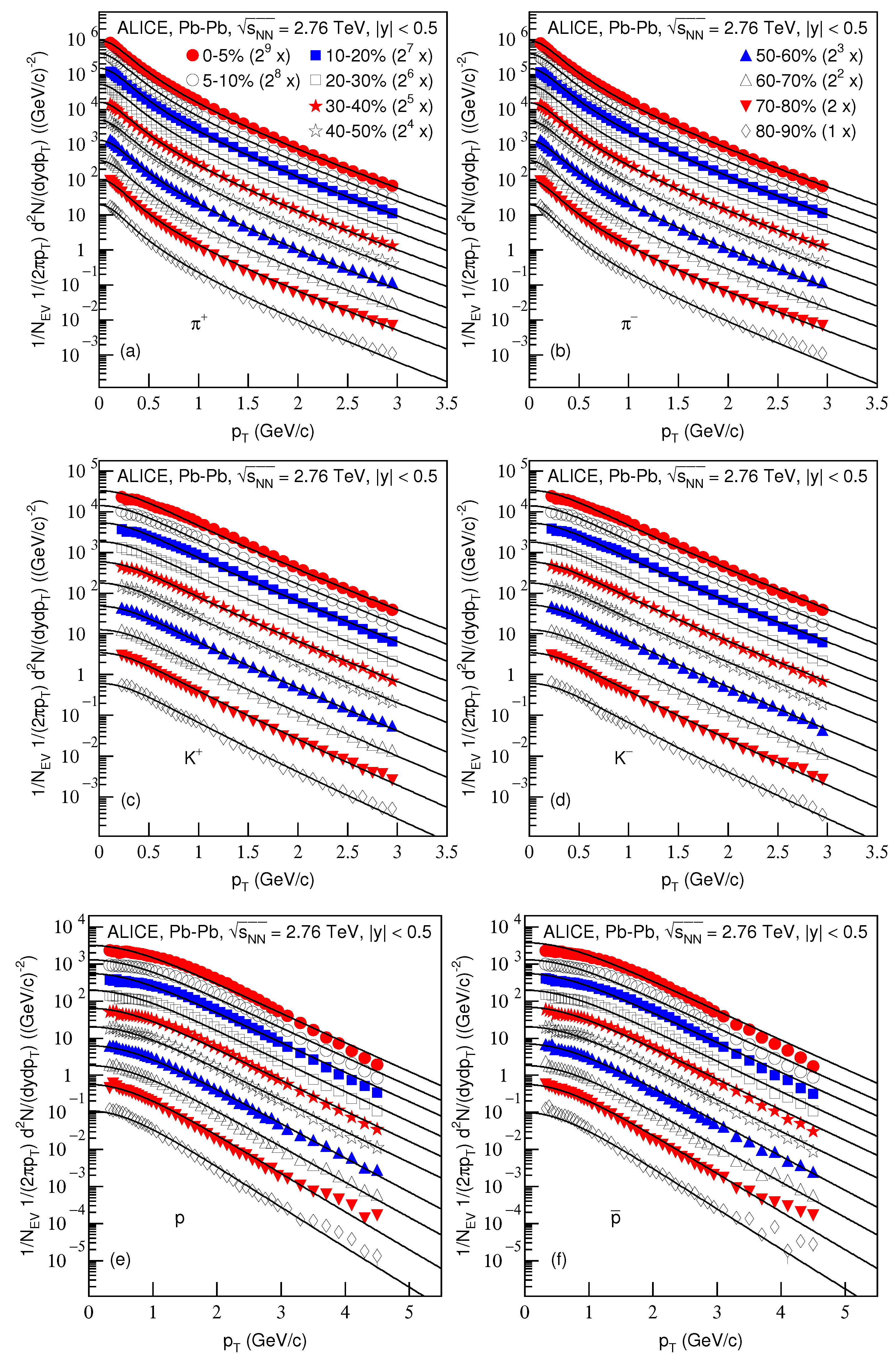
| Figure | Centrality | Particle | (GeV) | (c) | (fm/c) | /dof | (fm/c) |
|---|---|---|---|---|---|---|---|
| 1a | 0–5% | 203,000.0 ± 20,900.0 | 50.7/38 | ||||
| Pb–Pb | 5–10% | 170,000.0 ± 18,000.0 | 48.8/38 | ||||
| 10–20% | 130,000.0 ± 14,000.0 | 44.3/38 | |||||
| 20–30% | 90,000.0 ± 9900.0 | 50.5/38 | |||||
| 30–40% | 56,000.0 ± 6100.0 | 28.4/38 | |||||
| 40–50% | 34,000.0 ± 3700.0 | 19.5/38 | |||||
| 50–60% | 19,000.0 ± 2200.0 | 44.1/38 | |||||
| 60–70% | 10,000.0 ± 1200.0 | 43.5/38 | |||||
| 70–80% | 335.9/38 | ||||||
| 80–90% | 97.6/38 | ||||||
| 1b | 0–5% | 198,000.0 ± 20,600.0 | 68.6/38 | ||||
| Pb–Pb | 5–10% | 165,000.0 ± 17,000.0 | 58.2/38 | ||||
| 10–20% | 128,000.0 ± 13,000.0 | 43.7/38 | |||||
| 20–30% | 85,000.0 ± 9500.0 | 32.6/38 | |||||
| 30–40% | 54,000.0 ± 5900.0 | 22.2/38 | |||||
| 40–50% | 33,000.0 ± 3700.0 | 15.2/38 | |||||
| 50–60% | 19,000.0 ± 2200.0 | 25.0/38 | |||||
| 60–70% | 10,000.0 ± 1200.0 | 45.0/38 | |||||
| 70–80% | 184.1/38 | ||||||
| 80–90% | 98.3/38 | ||||||
| 1c | 0–5% | 87.9/33 | |||||
| Pb–Pb | 5–10% | 68.7/33 | |||||
| 10–20% | 58.2/33 | ||||||
| 20–30% | 40.2/33 | ||||||
| 30–40% | 18.5/33 | ||||||
| 40–50% | 14.9/33 | ||||||
| 50–60% | 24.9/33 | ||||||
| 60–70% | 20.8/33 | ||||||
| 70–80% | 92.5/33 | ||||||
| 80–90% | 50.3/33 | ||||||
| 1d | 0–5% | 10,100.0 ± 1100.0 | 58.3/33 | ||||
| Pb–Pb | 5–10% | 55.3/33 | |||||
| 10–20% | 46.7/33 | ||||||
| 20–30% | 25.3/33 | ||||||
| 30–40% | 13.3/33 | ||||||
| 40–50% | 14.8/33 | ||||||
| 50–60% | 13.4/33 | ||||||
| 60–70% | 25.8/33 | ||||||
| 70–80% | 95.0/33 | ||||||
| 80–90% | 66.7/33 | ||||||
| 1e | 0–5% | p | 243.0/39 | ||||
| Pb–Pb | 5–10% | 238.1/39 | |||||
| 10–20% | 160.8/39 | ||||||
| 20–30% | 120.9/39 | ||||||
| 30–40% | 87.9/39 | ||||||
| 40–50% | 68.1/39 | ||||||
| 50–60% | 53.4/39 | ||||||
| 60–70% | 101.5/39 | ||||||
| 70–80% | 222.7/39 | ||||||
| 80–90% | 95.6/39 | ||||||
| 1f | 0–5% | 174.0/39 | |||||
| Pb–Pb | 5–10% | 197.0/39 | |||||
| 10–20% | 143.6/39 | ||||||
| 20–30% | 106.2/39 | ||||||
| 30–40% | 81.8/39 | ||||||
| 40–50% | 101/39 | ||||||
| 50–60% | 47.0/39 | ||||||
| 60–70% | 92.1/39 | ||||||
| 70–80% | 144.1/39 | ||||||
| 80–90% | 115.1/39 | ||||||
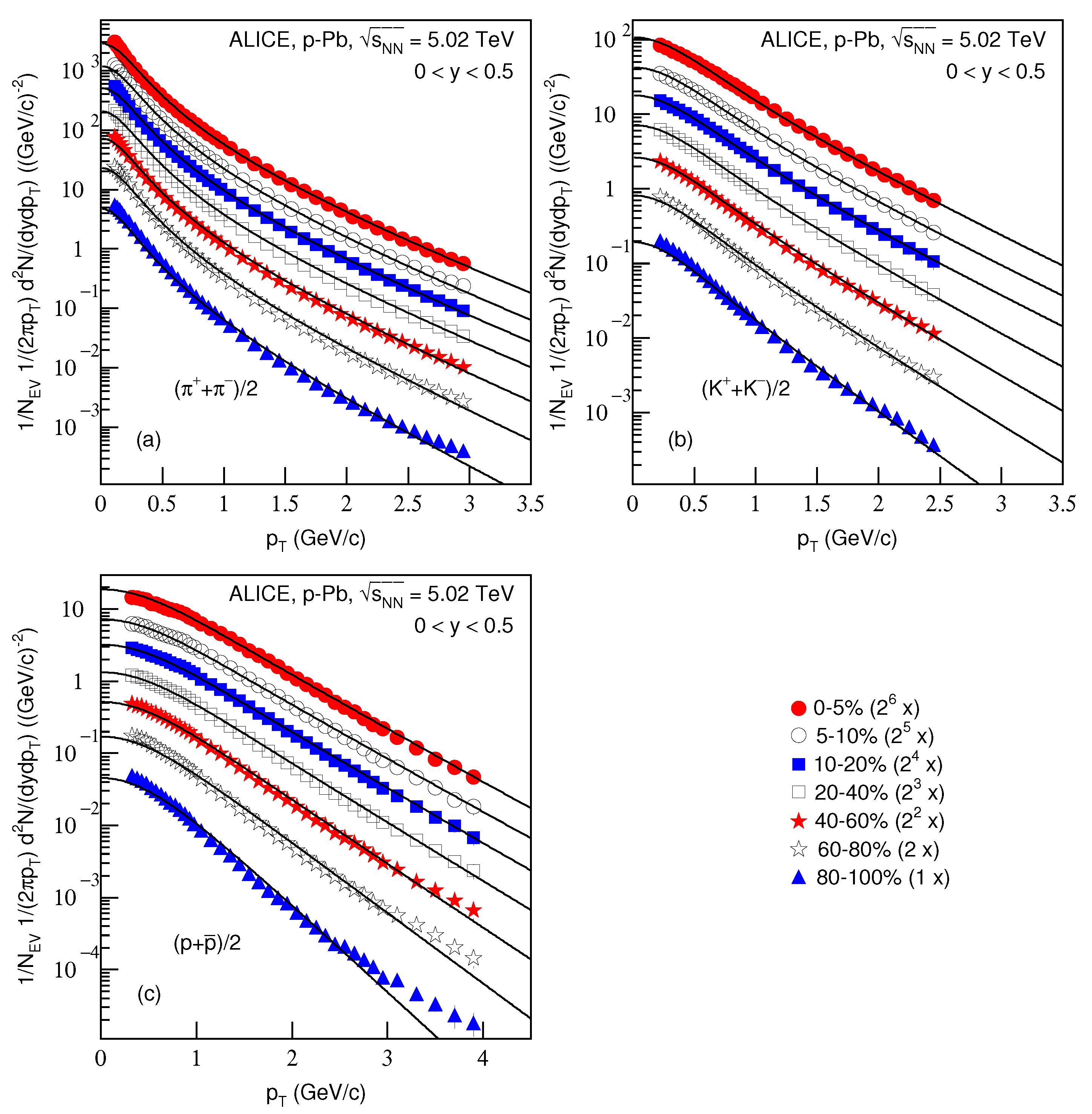
| 3a | 0–5% | ( | 163,500.0 ± 22,250.0 | 78.1/38 | |||
| p–Pb | 5–10% | 143,500.0 ± 19,680.0 | 62.3/38 | ||||
| 10–20% | 123,500.0 ± 16,550.0 | 82.3/38 | |||||
| 20–40% | 103,500.0 ± 15,500.0 | 170.6/38 | |||||
| 40–60% | 72,000.0 ± 10,650.0 | 183.1/38 | |||||
| 60–80% | 47,000.0 ± 6200.0 | 277.2/38 | |||||
| 80–100% | 22,000.0 ± 2305.0 | 516.5/38 | |||||
| 3b | 0–5% | ( | 12,000.0 ± 1805.0 | 15.8/28 | |||
| p–Pb | 5–10% | 5.7/28 | |||||
| 10–20% | 2.7/28 | ||||||
| 20–40% | 7.4/28 | ||||||
| 40–60% | 35.0/28 | ||||||
| 60–80% | 50.0/28 | ||||||
| 80–100% | 125.9/28 | ||||||
| 3c | 0–5% | ( | 41.8/36 | ||||
| p–Pb | 5–10% | 26.7/36 | |||||
| 10–20% | 21.3/36 | ||||||
| 20–40% | 37.6/36 | ||||||
| 40–60% | 57.7/36 | ||||||
| 60–80% | 116.1/36 | ||||||
| 80–100% | 192.5/36 | ||||||
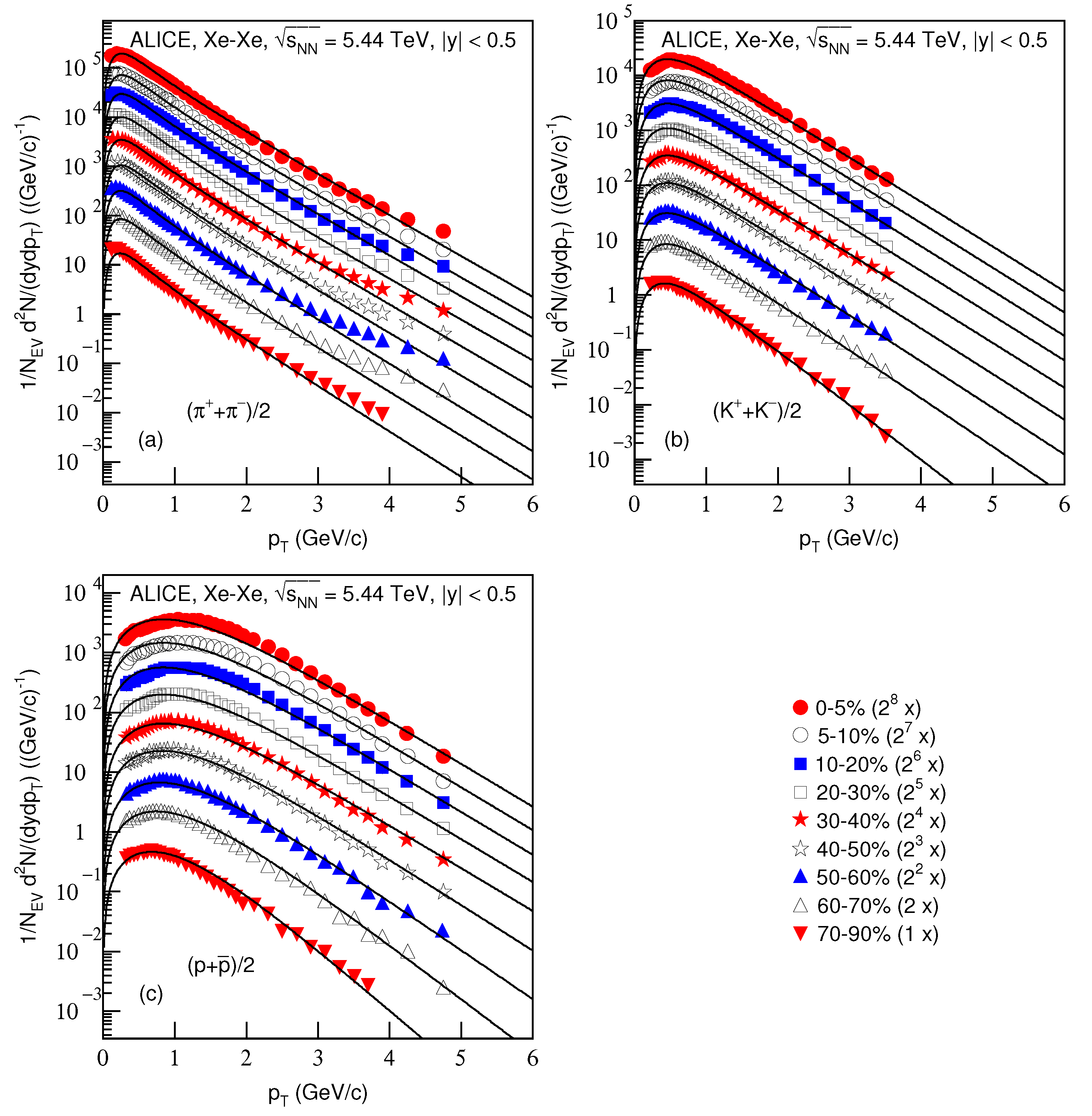
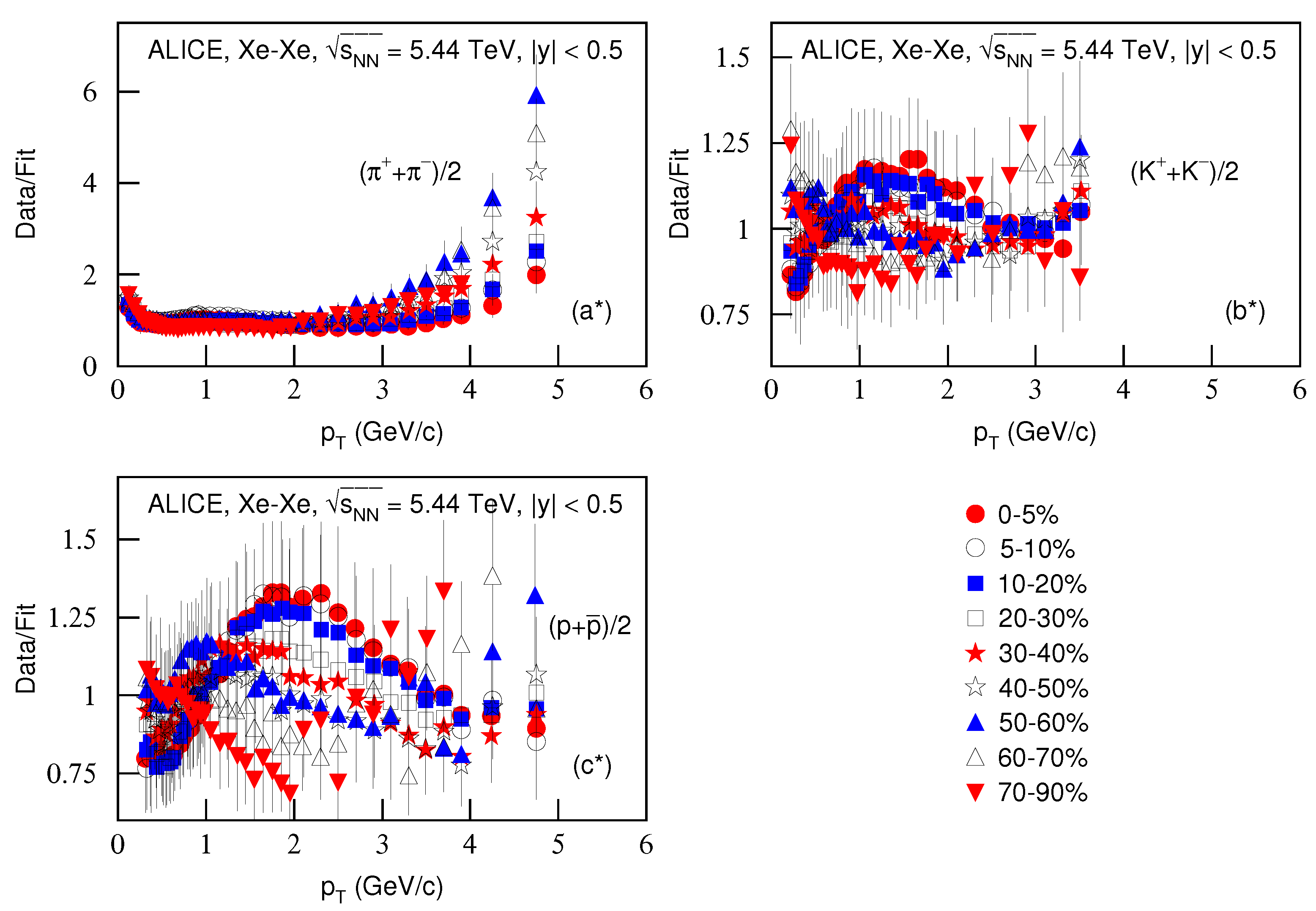
| 5a | 0–5% | ( | 67,892.5 ± 8920.0 | 19.5/38 | |||
| Xe–Xe | 5–10% | 49,892.5 ± 6044.0 | 19.2/38 | ||||
| 10–20% | 41,392.5 ± 4678.0 | 23.9/38 | |||||
| 20–30% | 27,892.5 ± 3462.0 | 40.6/38 | |||||
| 30–40% | 20,392.5 ± 2569.0 | 42.4/38 | |||||
| 40–50% | 13,142.5 ± 1581.0 | 53.0/38 | |||||
| 50–60% | 109.1/38 | ||||||
| 60–70% | 79.8/38 | ||||||
| 70–90% | 69.3/38 | ||||||
| 5b | 0–5% | ( | 18.1/30 | ||||
| Xe–Xe | 5–10% | 13.5/30 | |||||
| 10–20% | 10.5/30 | ||||||
| 20–30% | 5.4/30 | ||||||
| 30–40% | 3.4/30 | ||||||
| 40–50% | 5.1/30 | ||||||
| 50–60% | 5.4/30 | ||||||
| 60–70% | 13.8/30 | ||||||
| 70–90% | 20.2/30 | ||||||
| 5c | 0–5% | ( | 37.9/32 | ||||
| Xe–Xe | 5–10% | 37.6/32 | |||||
| 10–20% | 30.6/32 | ||||||
| 20–30% | 19.4/32 | ||||||
| 30–40% | 14.1/32 | ||||||
| 40–50% | 11.0/32 | ||||||
| 50–60% | 13.8/32 | ||||||
| 60–70% | 17.5/32 | ||||||
| 70–90% | 41.7/29 |
| Figure | Energy (TeV) | Particle | (GeV) | (c) | (fm/c) | /dof | (fm/c) |
|---|---|---|---|---|---|---|---|
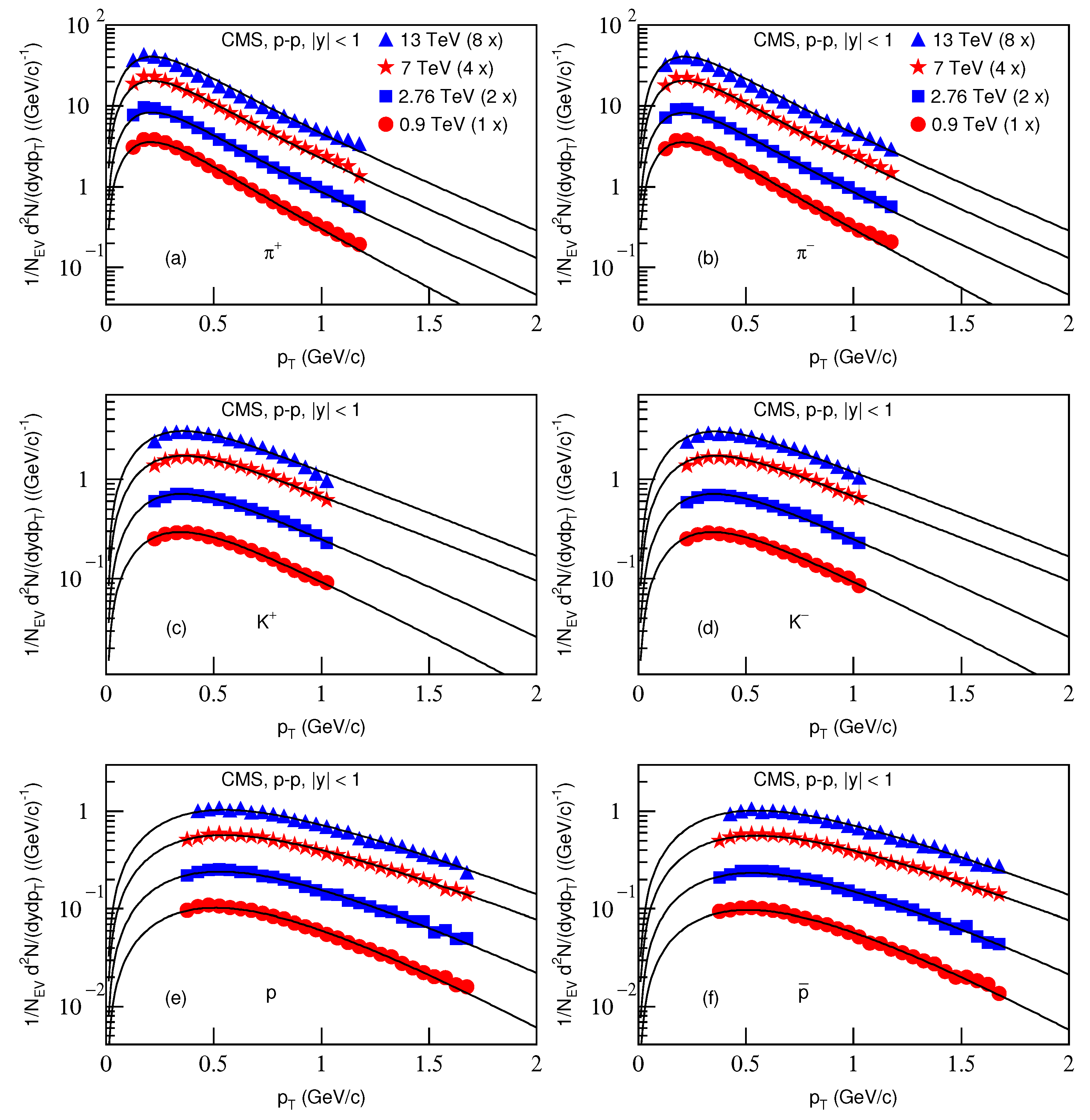
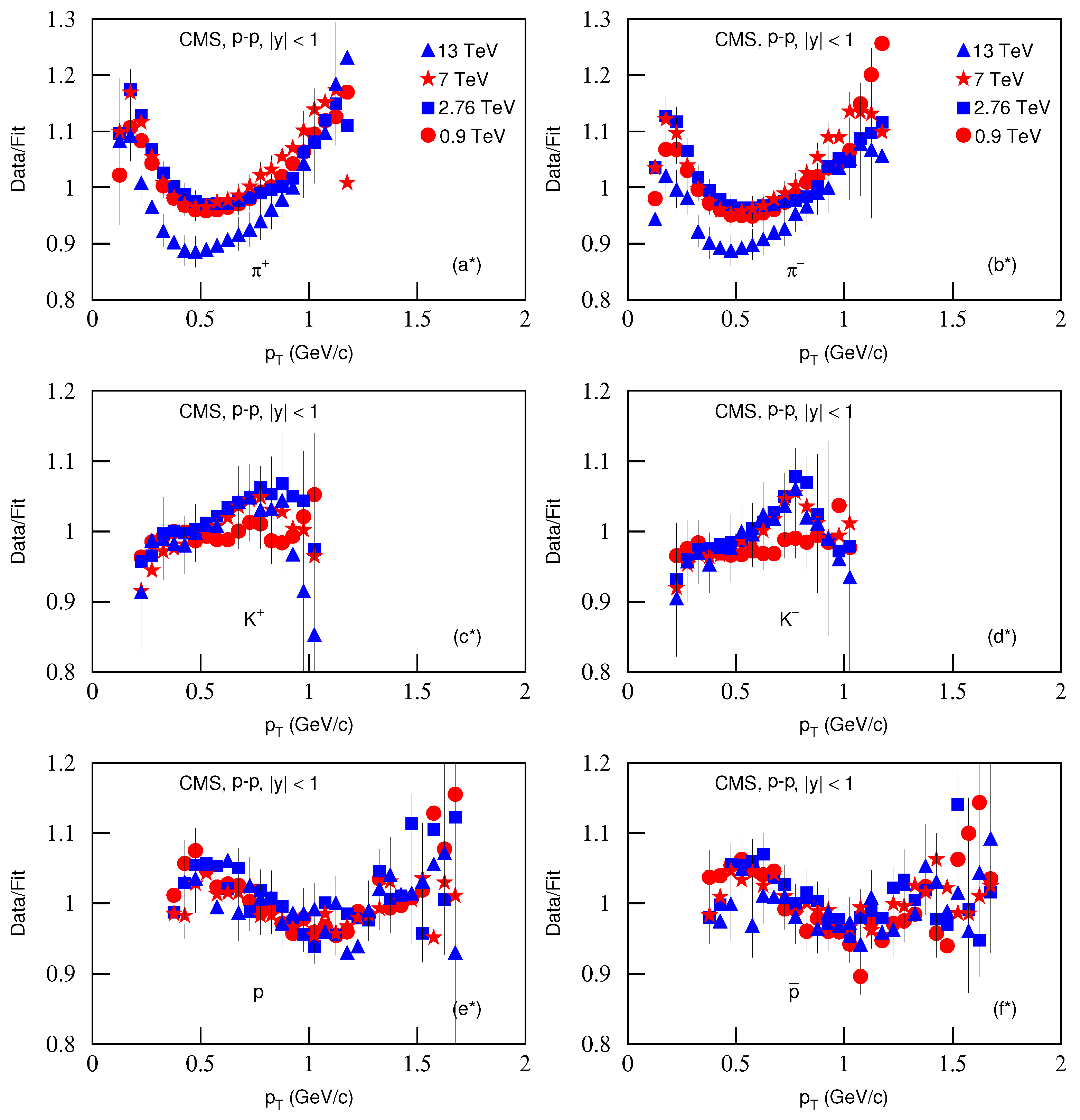
| 7a | 0.9 | 10,785.0 ± 1110.0 | 84.9/19 | ||||
| p–p | 2.76 | 12,785.0 ± 1300.0 | 105.3/19 | ||||
| 7 | 15,785.0 ± 1590.0 | 120.3/19 | |||||
| 13 | 15,785.0 ±1585.0 | 132.7/19 | |||||
| 7b | 0.9 | 10,725.0 ± 1110.0 | 117.9/19 | ||||
| p–p | 2.76 | 12,705.0 ± 1300.0 | 85.7/19 | ||||
| 7 | 15,815.0 ± 1590.0 | 116.0/19 | |||||
| 13 | 15,785.0 ± 1585.0 | 113.4/19 | |||||
| 7c | 0.9 | 3.3/14 | |||||
| p–p | 2.76 | 21.2/14 | |||||
| 7 | 20.2/14 | ||||||
| 13 | 5.2/14 | ||||||
| 7d | 0.9 | 16.7/14 | |||||
| p–p | 2.76 | 23.3/14 | |||||
| 7 | 22.9/14 | ||||||
| 13 | 6.5/14 | ||||||
| 7e | 0.9 | p | 37.9/24 | ||||
| p–p | 2.76 | 48.9/24 | |||||
| 7 | 21.2/24 | ||||||
| 13 | 15.3/23 | ||||||
| 7f | 0.9 | 66.8/24 | |||||
| p–p | 2.76 | 37.9/24 | |||||
| 7 | 23.4/24 | ||||||
| 13 | 11.9/23 | ||||||
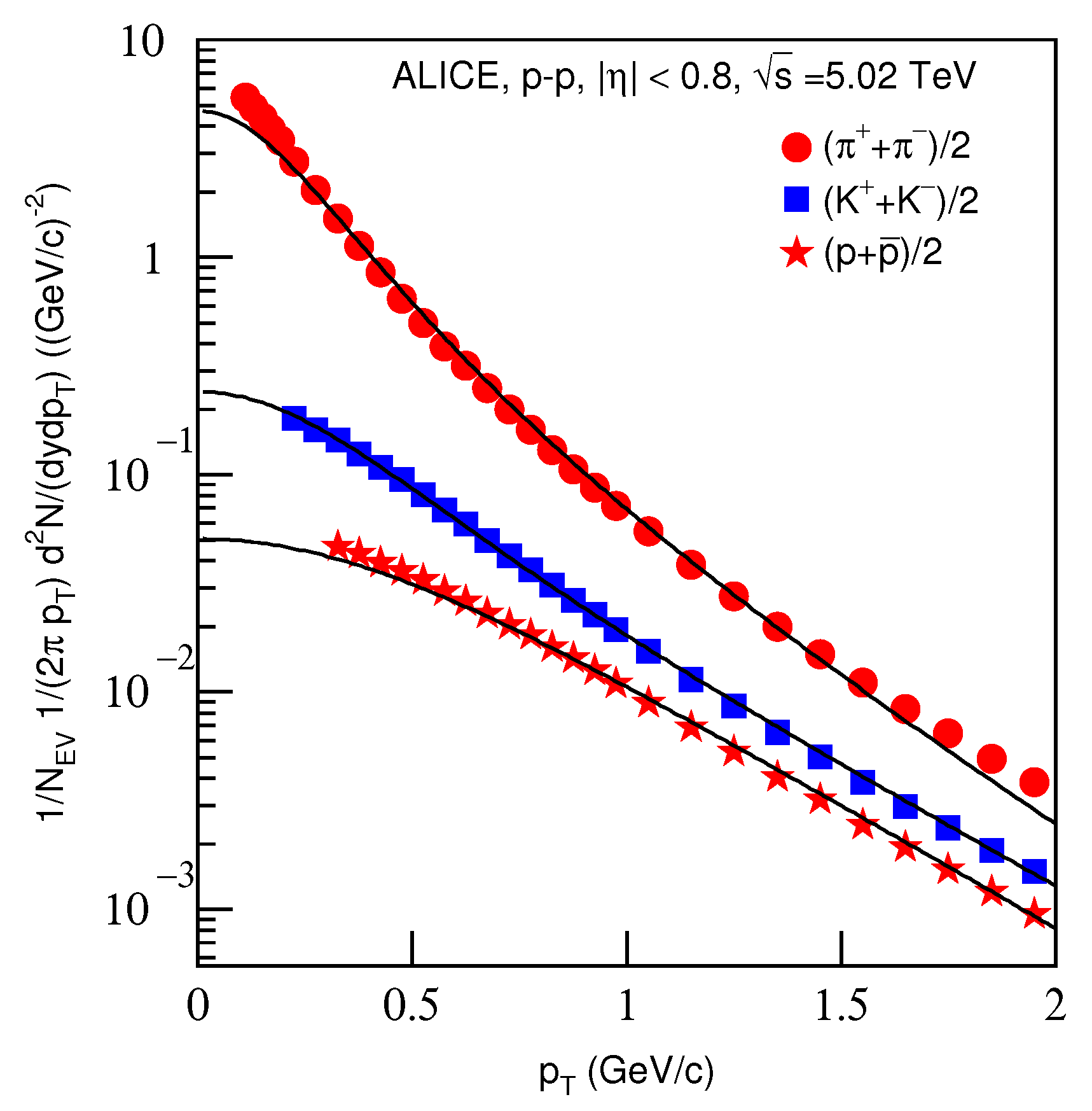
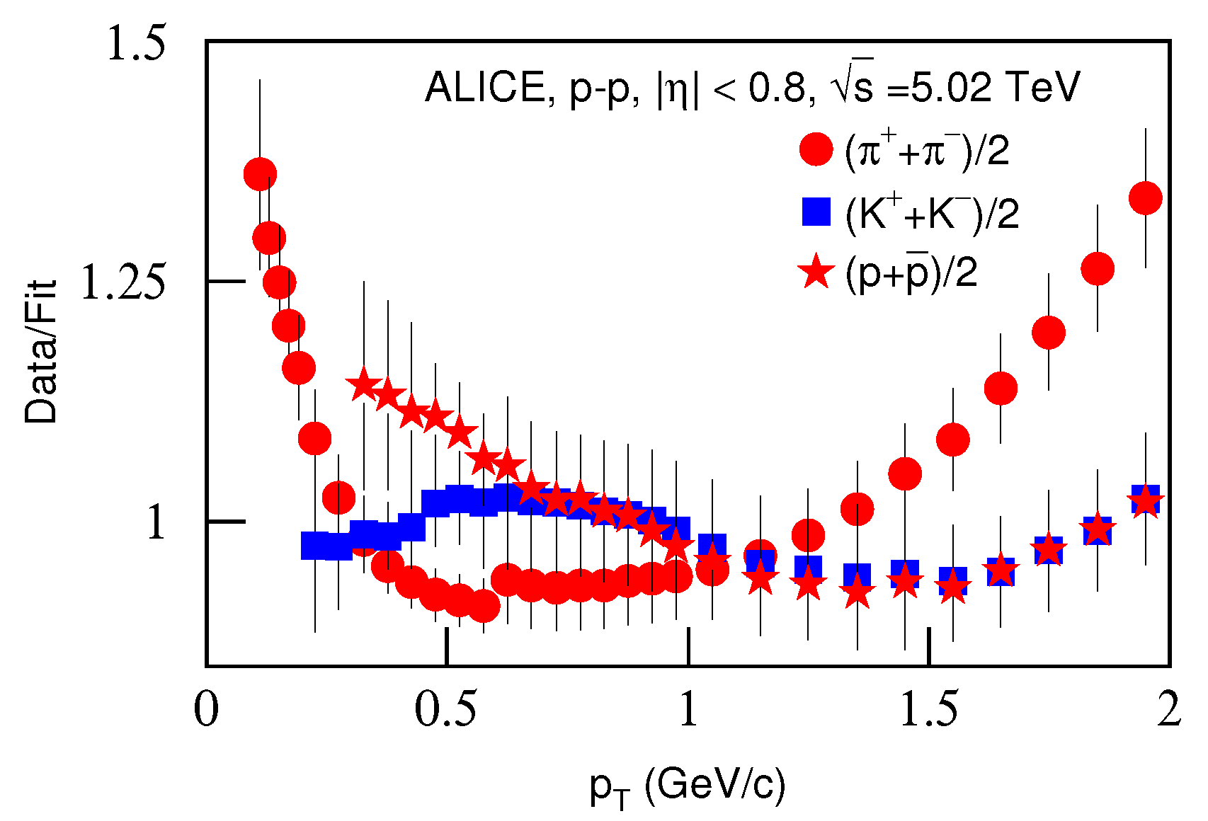
| 9 | 5.02 | ( | 11,242.5 ± 1055.0 | 187.6/28 | |||
| ( | 13.7/23 | ||||||
| ( | 23.5/21 |
| Figure | Centrality | b (fm) | (fm/c) | (fm/c) |
|---|---|---|---|---|
| 14a | 0–5% | 2.117 | ||
| Pb–Pb | 5–10% | 3.867 | ||
| 10–20% | 5.468 | |||
| 20–30% | 7.083 | |||
| 30–40% | 8.391 | |||
| 40–50% | 9.514 | |||
| 50–60% | 10.521 | |||
| 60–70% | 11.443 | |||
| 70–80% | 12.293 | |||
| 80–90% | 13.087 | |||
| 14a | 0–5% | 1.237 | ||
| p–Pb | 5–10% | 2.258 | ||
| 10–20% | 3.196 | |||
| 20–40% | 4.520 | |||
| 40–60% | 5.853 | |||
| 60–80% | 6.935 | |||
| 80–100% | 7.866 | |||
| 14a | 0–5% | 1.817 | ||
| Xe–Xe | 5–10% | 3.320 | ||
| 10–20% | 4.698 | |||
| 20–30% | 6.086 | |||
| 30–40% | 7.209 | |||
| 40–50% | 8.179 | |||
| 50–60% | 9.042 | |||
| 60–70% | 9.829 | |||
| 70–90% | 10.900 |
| Figure | Energy (TeV) | (fm/c) | (fm/c) |
|---|---|---|---|
| 14b | 0.9 | ||
| p–p | 2.76 | ||
| 5.02 | |||
| 7 | |||
| 13 | |||
| Pb–Pb | 2.76 | ||
| p–Pb | 5.02 | ||
| Xe–Xe | 5.44 |
Publisher’s Note: MDPI stays neutral with regard to jurisdictional claims in published maps and institutional affiliations. |
© 2021 by the authors. Licensee MDPI, Basel, Switzerland. This article is an open access article distributed under the terms and conditions of the Creative Commons Attribution (CC BY) license (https://creativecommons.org/licenses/by/4.0/).
Share and Cite
Lao, H.-L.; Liu, F.-H.; Ma, B.-Q. Analyzing Transverse Momentum Spectra of Pions, Kaons and Protons in p–p, p–A and A–A Collisions via the Blast-Wave Model with Fluctuations. Entropy 2021, 23, 803. https://doi.org/10.3390/e23070803
Lao H-L, Liu F-H, Ma B-Q. Analyzing Transverse Momentum Spectra of Pions, Kaons and Protons in p–p, p–A and A–A Collisions via the Blast-Wave Model with Fluctuations. Entropy. 2021; 23(7):803. https://doi.org/10.3390/e23070803
Chicago/Turabian StyleLao, Hai-Ling, Fu-Hu Liu, and Bo-Qiang Ma. 2021. "Analyzing Transverse Momentum Spectra of Pions, Kaons and Protons in p–p, p–A and A–A Collisions via the Blast-Wave Model with Fluctuations" Entropy 23, no. 7: 803. https://doi.org/10.3390/e23070803