Melodies as Maximally Disordered Systems under Macroscopic Constraints with Musical Meaning


Abstract
:
1. Introduction
2. Microscopic Representation and Macroscopic Observables of Intervals
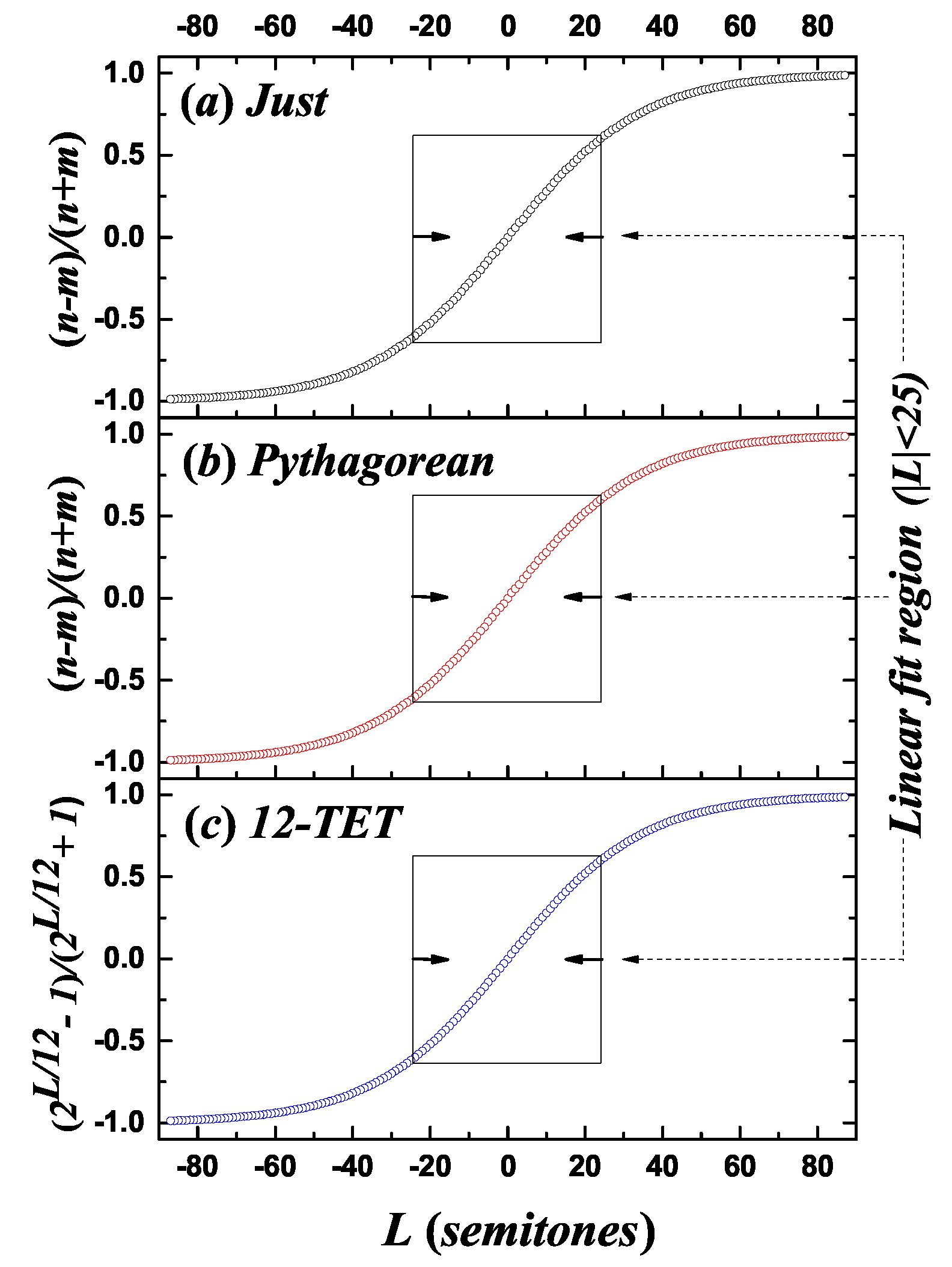
2.1. Interval Size and Its Relation to the Fundamental Frequency of Pitches
- In the just scale, with a determination coefficient ;
- In the Pythagorean scale, with ;
- In the 12-TET, .
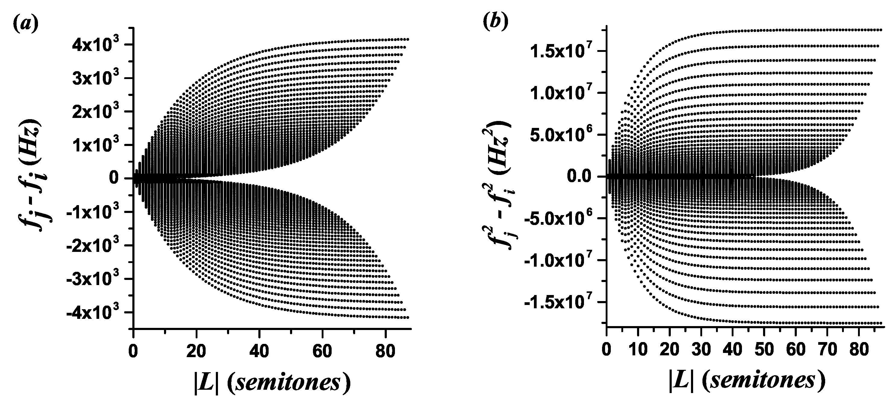
- For the just scale, with a determination coefficient ;
- For the Pythagorean scale, with ;
- For the 12-TET scale, with .
2.2. Expected Values with Musical Meaning
2.3. Transposition Process
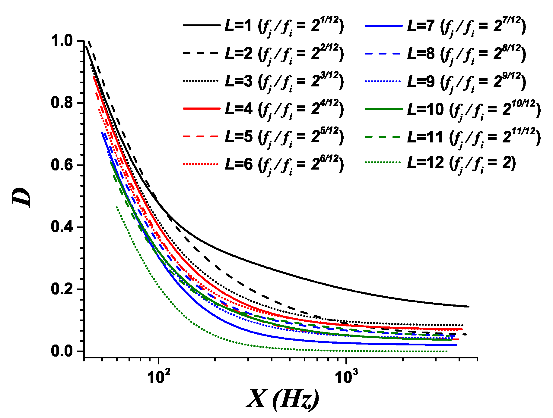
2.4. Distinguishability of Pairs of Pitches
3. Connection with Tonal Consonance
3.1. Measuring the Dissonance Levels of Intervals
3.2. Expected Values of the Dissonance Levels Associated to Intervals
4. Melody and Expected Values of Melodic Intervals
4.1. Concerning Melody
4.2. Expected Values of Melodic Intervals
5. Materials and Methods: An Application to Melodic Lines
5.1. Selection of Melodic Lines
- Brandenburg Concerto No. 3 in G Major BWV 1048. Johann Sebastian Bach: Polyphonic concerto for 11 musical instruments (three violins, three violas, three cellos, violone, and harpsichord).
- Missa Super Dixit Maria. Hans Leo Hassler: Polyphonic composition for four voices (soprano, contralto, tenor, and bass).
- First movement of the Partita in A Minor BWV 1013. Johann Sebastian Bach: This piece has just one melodic line for a flute.
- Piccolo Concerto RV444. Antonio Vivaldi (arrangement by Gustav Anderson): We selected the piccolo melodic line, owing to its rich melodic content.
- Sonata KV 545. Wolfgang Amadeus Mozart: We selected the melodic line for the right hand of this piano sonata, assuming that it drives the melodic content.
- Suite No. 1 in G Major BWV 1007 and Suite No. 2 in D Minor BWV 1008. Johann Sebastian Bach: The melodic lines of these pieces written for cello contain mainly successive pitches. In the cases of the few simultaneous pitches, the continuation of the melodic lines was assumed in the direction of the highest pitch.
5.2. Procedure to Obtain the Probability and the Cumulative Distributions
- The MIDI files were generated from scores. Only successive pitches without rests between them were considered.
- The MIDI information was transformed into frequencies using the 12-TET scale with Hz. Supplementary Spreadsheet S1 contains the data and in Hz, corresponding to the melodic intervals of each melodic line.
- The PDs were obtained in three different cases:
- -
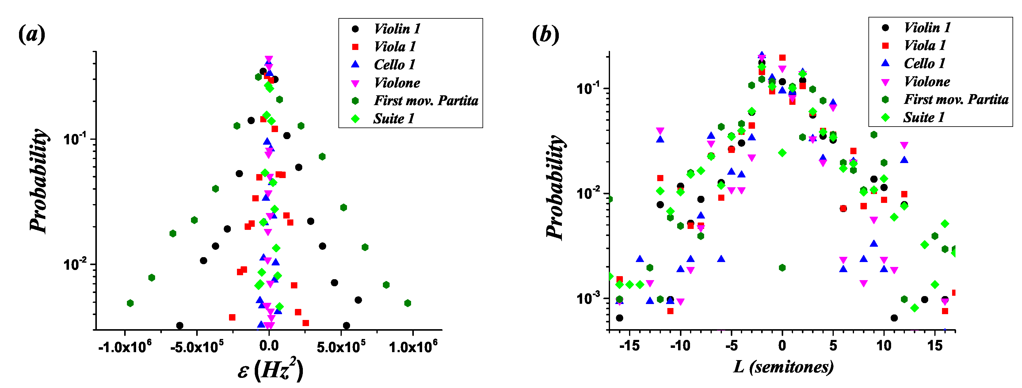
- Case 1: and not distinguishing between ascending and descending intervals. The complementary cumulative distribution (CCD) was also obtained.
- -
- Case 2: and for two different sets of intervals: Ascending and unisons, and descending and unisons. The CCD was also obtained for each set.
- -
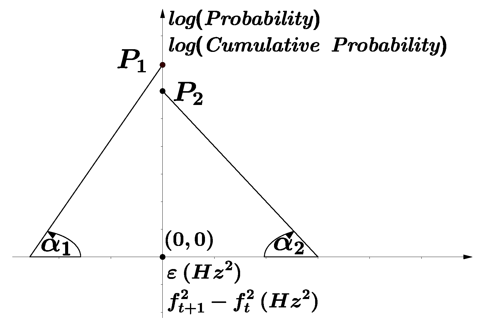
- Case 3: for the set of ascending, descending, and unison intervals together. In this case, the sign of the descending intervals was considered as negative. The reason for only using the quantity is the quality of the experimental fits obtained in the two previous analyses for both quantities, and even more relevantly that the distinguishability analysis shows that has the best resolution properties for the case of 24 semitones in the 12-TET scale (see Table 1), which is the relevant range for melodic intervals in the analyzed melodic lines. The CCD was employed for the branch of the PD that contains the ascending intervals, and the cumulative distribution (CD) was utilized for the branch that contains the descending intervals.
- Because the number of melodic intervals in the studied melodic lines is at most one order of magnitude larger than the total number of possible pairs of successive pitches generated by the same ambitus (the range between the lowest and highest pitches) of the original melodic line, the PDs were constructed using histograms, in order to capture significant probabilities. Supplementary Table S3 shows the number of intervals of each melodic line, the number of ascending intervals, descending ones, and unisons, and the corresponding ambitus.
- As the number of possible melodic intervals for any melodic line is finite, independently of its length, the bin width in the histograms will be moderately dependent on the number of melodic intervals. This condition is satisfied by the Sturges criterion [45], and thus, this criterion was used to determine the bin width.
- In the third case, when ascending and descending PDs were combined in the same distribution for the quantity , the bin width was taken as the average of those obtained separately using the Sturges criterion for ascending and descending distributions. The average bins were symmetrically located to the left and right, starting from the point .
- In the experimental analysis, the contribution of unisons in the histograms is important for ascending intervals as well as descending ones, with different right-hand and left-hand limits at 0. In addition, if we attempt to split the unisons into the ascending and descending parts, this procedure reduces the determination coefficient of the fits for the histograms to an exponential function [46]. Hence, all unisons were included in the ascending part as well as the descending one, and then a correction of this double count was carried out in the procedure to obtain the expected values. In the histograms, the descending intervals are contained inside the bins labeled from 1 to (from left to right), and the ascending ones inside those labeled from to N (from left to right). Hence, all unisons have been taken into account inside the bin labeled as well as that labelled . Notice that N is an even number.
6. Results and Discussion
6.1. Experimental Results and Analysis
6.2. Shannon Entropy of Melodic Intervals in Melodic Lines
6.3. Statistical Model for Melodic Lines: Relative Entropy Minimization under Macroscopic Constraints
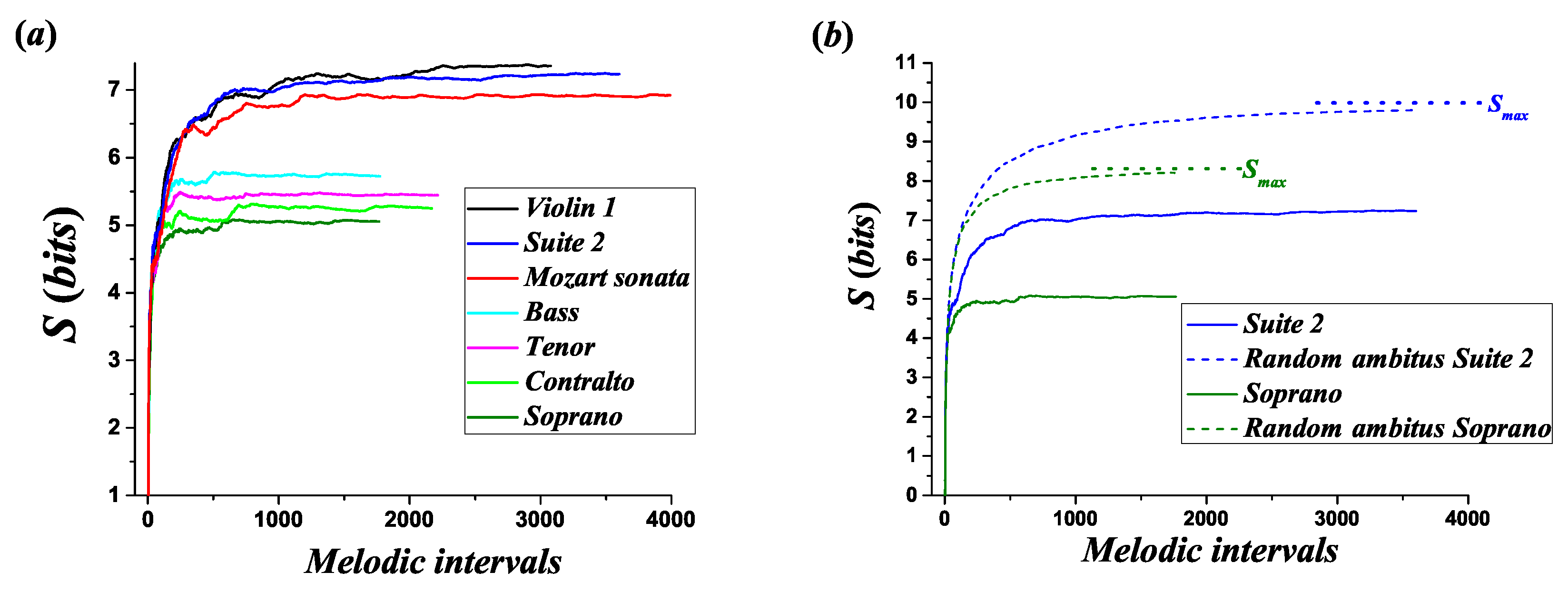
- Different registers of musical instruments and human voices can be distinguished using the Lagrange multiplier , allowing, for example, to discriminate between the same melodic line played in different parts of the register (a transposition). An example of a transposition is given in the Brandenburg Concerto No. 3 BWV 1048 by J. S. Bach, in which the harpsichord plays the same melodic line as the violone but transposed one octave higher (the fundamental frequency ratio of the transposition is equal to 2): While the entropy evolution in these melodic lines is the same, there is a change in the exponential decay parameters, characterized by the values of the Lagrange multipliers (see Table 2), and the numerical values of the expected values are related as:in agreement with the properties derived above for transposition processes (Equation (15)).
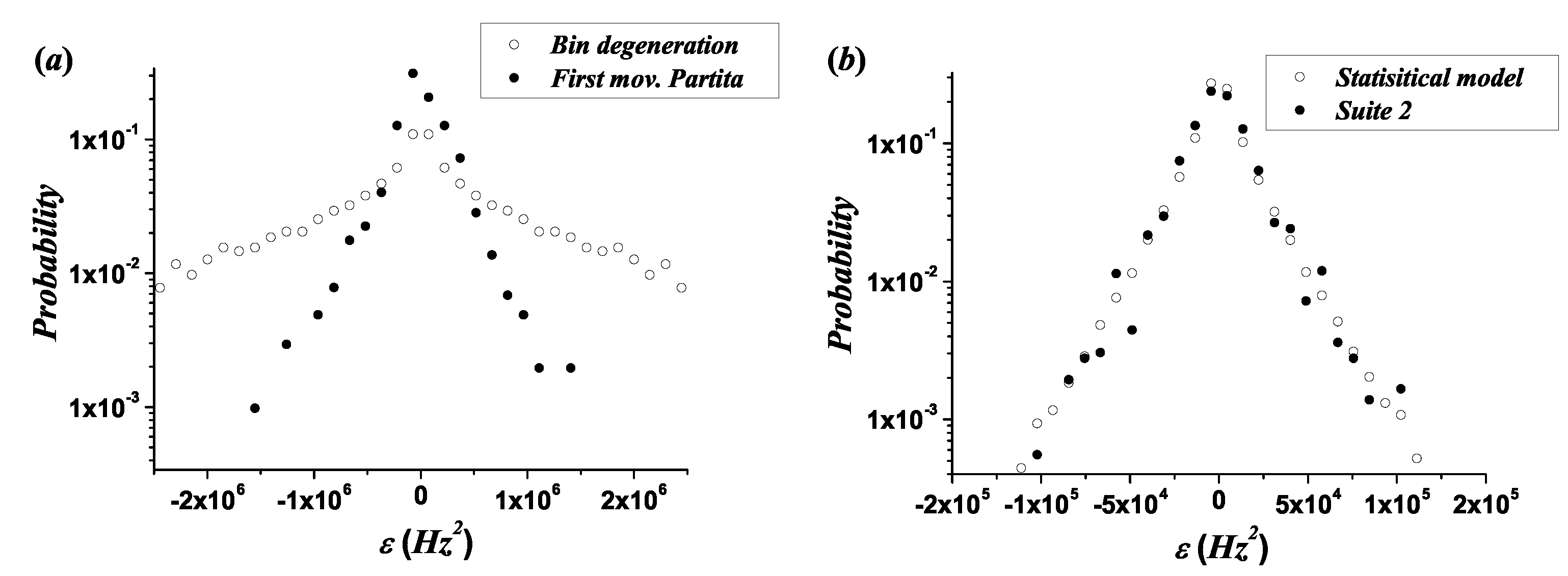
- With respect to the quantitative results of the model, the orders of magnitude of the fit parameters of the statistical model are in agreement with the corresponding results of the experimental fits. For each melodic line, Supplementary Table S8 contains the fit parameters to discontinuous asymmetric Laplace distributions, generated from the statistical model results. The average relative error in the histograms for the amplitude of the exponential distributions is , and that for the decay coefficient is . In the cases of the CD and CCD, the average errors of the amplitude and the decay coefficient are and , respectively. Supplementary Table S9 contains the values of these errors for each melodic line.
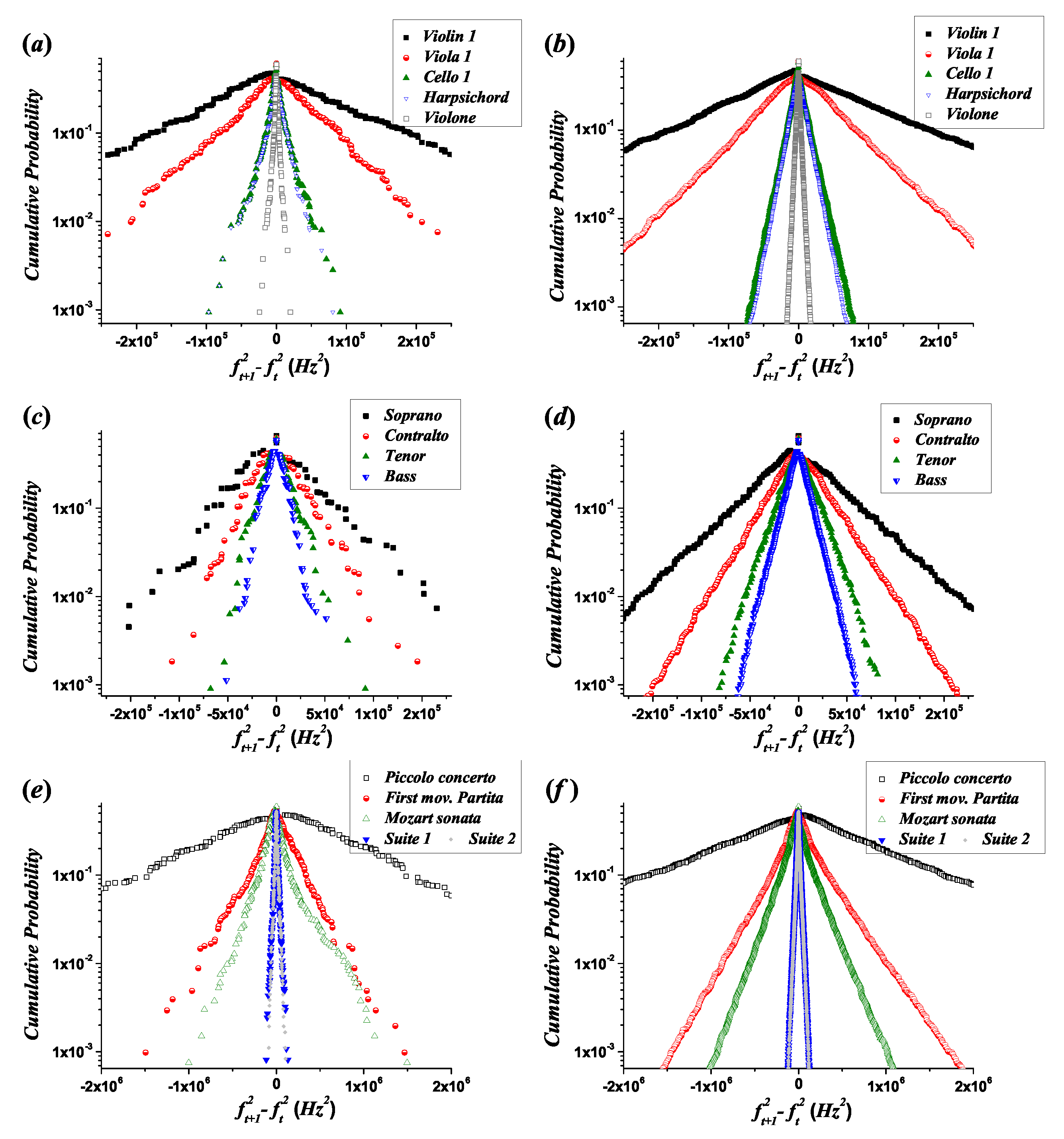
- In most cases ( of the melodic lines), Equation (35) takes positive values (corresponding to negative values of ), and takes negative values (see Supplementary Table S3). This behavior is consistent with the asymmetry represented in Figure 4, in the sense that the magnitudes of ascending intervals are expected to be larger than those of descending ones, and the total number of descending intervals must be larger than that of ascending ones. Negative values of and lead to different decay coefficients and different intercept points with the ordinate axis for the ascending and descending branches, which can be observed in the experimental fits of the CD and CCD through the comparison of the corresponding coefficients, and (see Supplementary Table S5). Figure 6 was created with the purpose of magnifying these particular asymmetries: and (implying that ). The two exceptions are the Piccolo Concerto RV444 of Antonio Vivaldi, where and , and the melodic line of the tenor voice in Missa Super Dixit Maria, where and .
- Because the difference between and is between one and two orders of magnitude (i.e., the decay coefficients have the same order of magnitude), and the bin width selection affects the measure of the decay parameters, the asymmetry in the values of the decay coefficients is better observed in the cumulative distributions than in the histograms.
- Because in Figure 6, the limit of the CD (constructed for descending intervals) when represents the probability of a value slightly smaller than 0, and in the CCD (constructed for ascending intervals), when represents the probability of a value slightly larger than 0, the asymmetry . This result can be observed in Figure 9 and represents the difference in the amplitudes of the exponential decay for the CD and CCD. In most cases, except for the Piccolo Concerto RV444, , implying that . In the case of the Piccolo Concerto RV444, it holds that , implying that .
6.4. Transposition Processes and Mean Dissonance Level of Melodic Lines
7. Conclusions
Supplementary Materials
Author Contributions
Funding
Acknowledgments
Conflicts of Interest
References
- Zanette, D. Zipf’s law and the creation of musical context. Music. Sci. 2006, 10, 3–18. [Google Scholar] [CrossRef]
- Tymoczko, D. The geometry of musical chords. Science 2006, 313, 72–74. [Google Scholar] [CrossRef]
- Manaris, B.; Purewal, T.; McCormick, C. Progress towards recognizing and classifying beautiful music with computers MIDI encoded music and the Zipf Mandelbrot law. In Proceedings of the IEEE SoutheastCon 2002, Columbia, SC, USA, 5–7 April 2002. [Google Scholar] [CrossRef]
- Zipf, G. Human Behavior and the Principle of Least Effort; Addison-Wesley: Cambridge, MA, USA, 1949. [Google Scholar]
- Voss, P.; Troost, J. Ascending and Descending Melodic Intervals: Statistical Findings and Their Perceptual Relevance. Music Percept. Interdiscip. J. 1989, 6, 383–396. [Google Scholar] [CrossRef]
- Huron, D. A comparison of average pitch height and interval size in major- and minor-key themes: Evidence consistent with affect-related pitch prosody. Empir. Musicol. Rev. 2008, 3, 59–63. [Google Scholar] [CrossRef]
- Beltrán del Río, M.; Cocho, G.; Naumis, G. Universality in the tail of musical note rank distribution. Physica A 2008, 387, 5552–5560. [Google Scholar] [CrossRef]
- Liu, X.; Small, M.; Tse, C. Complex network structure of musical compositions: Algoritmic generation of appealing music. Physica A 2010, 389, 126–132. [Google Scholar] [CrossRef]
- Wu, D.; Kendrick, K.; Levitin, D.; Li, C.; Yao, D. Bach Is the Father of Harmony: Revealed by a 1/f Fluctuation Analysis across Musical Genres. PLoS ONE 2015, 10, e0142431. [Google Scholar] [CrossRef] [PubMed]
- Roederer, J. Acústica y psicoacústica de la música [The Physics and Psychophysics of Music]; Ricordi Americana S.A.E.C.: Buenos Aires, Argentina, 1997. [Google Scholar]
- Plomp, R.; Levelt, J. Tonal Consonance and Critical Band Width. J. Acoust. Soc. Am. 1965, 38, 548–560. [Google Scholar] [CrossRef]
- Useche, J.; Hurtado, R. Pitch Structure of Melodic Lines: An Interface between Physics and Perception. In Proceedings of the 33rd Annual Conference of the Cognitive Science Society, Boston, MA, USA, 20–23 July 2011. [Google Scholar] [CrossRef]
- Bowling, D.; Sundararajan, J.; Han, S.; Purves, D. Expression of Emotion in Eastern and Western Music Mirrors Vocalization. PLoS ONE 2012, 7, e31942. [Google Scholar] [CrossRef]
- Huron, D.; Davis, M. The Harmonic Minor Scale Provides an Optimum Way of Reducing Average Melodic Interval Size, Consistent with Sad Affect Cues. Empir. Musicol. Rev. 2012, 7, 103–117. [Google Scholar] [CrossRef]
- Moore, S. Interval Size and Affect: An Ethnomusicological Perspective. Empir. Musicol. Rev. 2012, 7, 138–143. [Google Scholar] [CrossRef]
- Temperley, D.; de Clercq, T. Statistical Analysis of Harmony and Melody in Rock Music. J. New Music Res. 2013, 42, 187–204. [Google Scholar] [CrossRef]
- Voss, R.; Clarke, J. ‘1/f noise’ in music and speech. Nature 1975, 258, 317–318. [Google Scholar] [CrossRef]
- Hennig, H. Synchronization in human musical rhythms and mutually interacting complex systems. Proc. Natl. Acad. Sci. USA 2014, 111, 12974–12979. [Google Scholar] [CrossRef] [PubMed] [Green Version]
- Niklasson, G.; Niklasson, M. Non-Gaussian distributions of melodic intervals in music: The Lévy-stable approximation. EPL Lett. J. Explor. Front. Phys. 2015, 112, 40003. [Google Scholar] [CrossRef]
- González, A.; Larralde, H.; Martínez, G.; Müller, M. Multiple scaling behaviour and nonlinear traits in music scores. R. Soc. Open Sci. 2017, 4, 171282. [Google Scholar] [CrossRef] [Green Version]
- Pinkerton, R. Information theory and melody. Sci. Am. 1956, 194, 77–86. [Google Scholar] [CrossRef]
- Youngblood, J. Style as information. J. Music Theory 1958, 2, 24–35. [Google Scholar] [CrossRef]
- Hiller, L.; Bean, C. Information theory analyses of four sonata expositions. J. Music Theory 1966, 10, 96–137. [Google Scholar] [CrossRef]
- Hiller, L.; Fuller, R. Structure and information in Webern’s Symphonie, Op. 21. J. Music Theory 1967, 11, 60–115. [Google Scholar] [CrossRef]
- Knopoff, L.; Hutchinson, W. Entropy as a measure of style: The influence of sample length. J. Music Theory 1983, 27, 75–97. [Google Scholar] [CrossRef]
- Dubnov, S.; Assayag, G.; El-Yaniv, R. Universal classification applied to musical sequences. In Proceedings of the 1998 International Computer Music Conference; ICMA: San Francisco, CA, USA, 1998; pp. 332–340. [Google Scholar]
- Manzara, L.; Witten, I.; James, M. On the Entropy of Music: An Experiment with Bach Chorales Melodies. Leonardo Music J. 1992, 2, 81–88. [Google Scholar] [CrossRef]
- Gündüz, G.; Gündüz, U. The mathematical analysis of the structure of some songs. Physica A 2005, 357, 565–592. [Google Scholar] [CrossRef]
- Triviño, J.; Morales, R. Using multi-attribute prediction suffix graphs to predict and generate music. Comput. Music J. 2001, 25, 62–79. [Google Scholar] [CrossRef]
- Cohen, J. Information theory and music. Behav. Sci. 1962, 7, 137–163. [Google Scholar] [CrossRef]
- Patel, A. Music, Language, and the Brain, 2nd ed.; Oxford University Press, Inc.: New York, NY, USA, 2008. [Google Scholar]
- Rossing, T. The Science of Sound, 2nd ed.; Addison-Wesley: Reading, MA, USA, 1990. [Google Scholar]
- Schön, D.; Regnault, P.; Ystad, S.; Besson, M. Sensory Consonance: An ERP Study. Music Percept. 2004, 23, 105–117. [Google Scholar] [CrossRef]
- Pain, H. The Physics of Vibrations and Waves, 6th ed.; John Wiley and Sons Ltd.: Hoboken, NJ, USA, 2005. [Google Scholar]
- Sethares, W. Local consonance and the relation between timbre and scales. J. Acoust. Soc. Am. 1993, 94, 1218–1228. [Google Scholar] [CrossRef]
- Sethares, W. Tuning, Timbre, Spectrum, Scale, 2nd ed.; Springer: London, UK, 2005. [Google Scholar]
- Aldwell, E.; Schachter, C. Harmony and Voice Leading, 2nd ed.; Harcourt Brace Jovanovich: San Diego, CA, USA, 1988. [Google Scholar]
- Sethares, W. Tuning, Timbre, Spectrum, Scale, 1st ed.; Springer: London, UK, 1998. [Google Scholar]
- Vassilakis, P. Perceptual and Physical Properties of Amplitude Fluctuation and Their Musical Musical Significance. Ph.D. Thesis, University of California, Los Angeles, CA, USA, 2001. [Google Scholar]
- Vassilakis, P.; Kendall, R. Psichoacoustic and cognitive aspects of auditory roughness: Definitions, models and applications. In Proceedings of the SPIE 7527, Human Vision and Electronic Imaging XV; Cognitive Science Society: Austin, TX, USA, 2010; Volume 7527. [Google Scholar] [CrossRef]
- Leman, M. Music and Schema Theory-Cognitive Foundations of Systematic Musicology; Springer: Berlin, Germany, 1995. [Google Scholar]
- Maher, T.; Berlyne, D. Verbal and exploratory responses to melodic musical intervals. Psychol. Music 1982, 10, 11–27. [Google Scholar] [CrossRef]
- Apel, W. Harvard Dictionary of Music, 2nd ed.; Harvard Press University: Cambridge, MA, USA, 1974. [Google Scholar]
- Huron, D. Sweet Anticipation: Music and the Psychology of Expectation; The MIT Press: Cambridge, MA, USA, 2006. [Google Scholar]
- Scott, D. Multivariate Density Estimation: Theory, Practice, and Visualization; John Wiley and Sons: Hoboken, NJ, USA, 1992. [Google Scholar]
- Useche, J. Aplicación del Análisis de Redes, el Formalismo de las Redes Complejas y la Mecánica Estadística al Estudio de la Música Clásica [Application of Network Analysis, the Complex Networks Framework, and Statistical Mechanics to the Study of Academic Music]. Master’s Thesis, Universidad Nacional de Colombia, Bogota, Colombia, 2012. [Google Scholar]
- Kotz, S.; Kozubowski, T.; Podgorski, K. The Laplace Distribution and Generalizations: A Revisit with Applications to Communications, Economics, Engineering, and Finance; Birkhaüser Boston: Boston, MA, USA, 2001. [Google Scholar]
- Cover, T.; Thomas, J. Elements of Information Theory; John Wiley and Sons: Hoboken, NJ, USA, 2006. [Google Scholar]
- Niven, R. Non-asymptotic thermodynamic ensembles. Europhys. Lett. 2009, 86, 20010. [Google Scholar] [CrossRef]


| Scale | Up to 24 Semitones | Up to 87 Semitones | ||
|---|---|---|---|---|
| Just | 52 for | 2 for | 208 for | 5 for |
| Pythagorean | 8 for | 0 for | 47 for | 2 for |
| 12-TET | 0 for | 0 for | 0 for | 0 for |
| Melodic Line | |||||||
|---|---|---|---|---|---|---|---|
| Violin 1 | 7.358 | 7.378 | 10.089 | 0.550 | −1.870 | 1.282 | 1.278 |
| Violin 2 | 7.213 | 7.234 | 10.000 | 0.570 | −0.189 | 1.215 | 1.211 |
| Violin 3 | 7.253 | 7.285 | 10.000 | 0.660 | −0.895 | 1.242 | 1.240 |
| Viola 1 | 6.941 | 6.953 | 9.615 | 1.330 | −1.860 | 1.339 | 1.333 |
| Viola 2 | 6.935 | 6.944 | 9.510 | 1.500 | −1.280 | 1.381 | 1.375 |
| Viola 3 | 7.022 | 7.053 | 9.716 | 1.540 | −2.200 | 1.364 | 1.357 |
| ⋆ Cello 1 | 6.888 | 6.904 | 9.716 | 6.300 | −18.700 | 2.795 | 2.788 |
| ⋆ Cello 2 | 6.884 | 6.899 | 9.716 | 6.400 | −17.200 | 2.797 | 2.790 |
| ⋆ Cello 3 | 6.862 | 6.879 | 9.716 | 6.500 | −15.100 | 2.816 | 2.812 |
| Violone | 6.779 | 6.796 | 9.716 | 30.000 | −34.000 | 4.900 | 4.917 |
| ⋆ Harpsichord | 6.779 | 6.796 | 9.716 | 7.400 | −4.200 | 2.596 | 2.598 |
| Soprano | 5.055 | 5.082 | 8.340 | 1.940 | −2.850 | 1.470 | 1.470 |
| Contralto | 5.247 | 5.313 | 8.644 | 3.250 | −6.800 | 1.591 | 1.591 |
| Tenor | 5.443 | 5.491 | 7.615 | 5.100 | −6.500 | 1.893 | 1.893 |
| Bass | 5.723 | 5.787 | 8.644 | 7.300 | 6.450 | 2.219 | 2.218 |
| ⋆ Suite 1 | 7.069 | 7.073 | 10.000 | 3.500 | −5.100 | 2.528 | 2.509 |
| ⋆ Suite 2 | 7.235 | 7.248 | 10.000 | 3.700 | −5.800 | 2.653 | 2.631 |
| Mozart sonata | 6.923 | 6.935 | 10.644 | 0.490 | −1.520 | 1.353 | 1.357 |
| First mov. Partita | 7.145 | 7.145 | 10.000 | 0.295 | −1.760 | 1.293 | 1.294 |
| ⋆ Piccolo concerto | 7.087 | 7.182 | 9.288 | 0.056 | 0.175 | 0.749 | 0.747 |
© 2019 by the authors. Licensee MDPI, Basel, Switzerland. This article is an open access article distributed under the terms and conditions of the Creative Commons Attribution (CC BY) license (http://creativecommons.org/licenses/by/4.0/).
Share and Cite
Useche, J.; Hurtado, R. Melodies as Maximally Disordered Systems under Macroscopic Constraints with Musical Meaning. Entropy 2019, 21, 532. https://doi.org/10.3390/e21050532
Useche J, Hurtado R. Melodies as Maximally Disordered Systems under Macroscopic Constraints with Musical Meaning. Entropy. 2019; 21(5):532. https://doi.org/10.3390/e21050532
Chicago/Turabian StyleUseche, Jorge, and Rafael Hurtado. 2019. "Melodies as Maximally Disordered Systems under Macroscopic Constraints with Musical Meaning" Entropy 21, no. 5: 532. https://doi.org/10.3390/e21050532