Wind Turbine Surface Defect Detection Method Based on YOLOv5s-L

Abstract

In order to solve the problems of low efficiency, time consumption and high costs in the detection of defects on wind turbine surfaces in industrial scenarios, an improved YOLOv5 algorithm for wind turbine surface defect detection is proposed, named YOLOv5s-L. Firstly, the C3 module of YOLOv5s is replaced with the C2f module, which is more abundant in gradient flow, to enhance the ability of feature extraction and feature fusion. Secondly, the Squeeze and Excitation (SE) module is embedded in the YOLOv5 Backbone network to filter out redundant feature information and retain important feature information. Thirdly, the weighted Bidirectional Feature Pyramid Network (BiFPN) is introduced to replace the FPN + PAN, which can achieve a higher level of feature fusion while keeping the weight light. Finally, the Focal Loss function is used to replace the CIOU Loss function of the YOLOv5 algorithm to optimize the training model and improve the accuracy of the algorithm. The experimental results show that, compared with the traditional YOLOv5 algorithm, the average precision mAP is improved by 1.9%, and the frame rate FPS can reach 145 F/s without increasing the model parameters; it can satisfy the requirements for real-time, accurate detection on mobile devices. This method provides effective support for surface defect detection of wind turbines and provides reference for intelligent wind farm operation and maintenance.

1. Introduction

In recent years, wind energy, as a renewable energy belonging to the same core type as solar energy, can effectively promote the sustainable development of cities and society, just like solar energy [1]. As the installed capacity of wind power in our country increases year by year, and as most wind turbines are located in remote open areas, the operation of wind turbines faces various threats, including severe dust storms, heavy snow and corrosive acid rain [2,3,4], which means the surface is prone to a large number of defects. Due to the high manufacturing cost of wind turbines, these defects will lead to complex and expensive maintenance problems and serious safety risks [5]. Therefore, the early and timely detection of defects on wind turbine surfaces is critical.

At present, the surface defect detection of wind turbines is mainly based on manual detection, which is inefficient and costly, and cannot guarantee the detection accuracy. The applicability of different non-destructive testing methods varies, mainly including ultrasonic testing [6], vibration analysis method [7], strain sensor [8], infrared imaging method [9], etc., but there are still issues like the difficulty of processing a large amount of collection data and the high maintenance cost of sensors and other equipment in the above detection methods. In addition, there is no effective detection of early, small defects.

As interest in deep learning has grown, machine learning tools have exploded in popularity. Cascade R-CNN and YOLOv5 became two-stage and one-stage optimal detection frameworks but are still facing multiple challenges [10]. Wang L et al. [11] proposed a two-stage method based on UAV images to automatically locate the surface cracks on wind turbine blades and detect their contours, but it cannot achieve a high accuracy and real-time detection. Dong Gang et al. [12] summarized the small target detection algorithms and pointed out that the small target detection accuracy is too low compared with the large target.

YOLO is one of the most widely used target detection algorithms with multiple versions. Because the entire channel of YOLO is a single network, it can be directly optimized for end-to-end detection performance, which is easier to implement and can train the entire image immediately [13]. In July 2020, Ultralytics released YOLOv5. The YOLOv5 network is divided into four parts: Input, Backbone, Neck and Head. The structure of the YOLOv5 is shown in Figure 1 and Improved YOLOv5 network structure in Figure 2. As the initial stage of image detection, the Input image will be automatically extracted with the CNN structure and then the feature image will be divided into the same area grid; the probability of the defect to be tested was predicted using the regression box, and the results were evaluated by confidence level. Backbone (Backbone network) uses deep convolution to extract features from different layers of images, mainly using the C3 module and spatial pyramid pooling (SPP). C3 consists of three standard convolution layers and N Bottleneck modules, which can learn the residual features to reduce computation and improve reasoning speed. SPP will extract feature information of different scales from the same or multiple feature maps, which is helpful to improve the detection accuracy. The Neck mainly consists of two parts, including the feature pyramid network (FPN) and path aggregation network (PAN). FPN transmits semantic information from top to bottom, while Pan transmits location information from bottom to top. Both of them realize the function of fusing different network layers’ Backbone information, which makes the model obtain more abundant feature information. As the final detection module, the Head consists of a series of convolution layers and full connection layers, which can transform the extracted features of the Backbone and Neck into the results of target detection, focusing on predicting different objects on feature maps of different sizes to achieve object classification and regression functions. As the final detection module, Head consists of a series of convolution layers and full connection layers, which can transform the extracted features of Backbone and Neck into the results of target detection, focusing on predicting different objects on feature maps of different sizes to achieve object classification and regression functions. Since YOLO does not use a separate network to extract candidate regions, it performs better than Fast R-CNN in terms of processing time. Wang et al. [14] carried out the YOLOv5 algorithm to detect abnormal flow on the vibrating screen, so as to assist field engineers to better discover the fluid movement on the vibrating screen in the actual operation. Yu et al. [15] proposed a TR-YOLOv5s network and down-sampling principle based on YOLOv5, which greatly improves the detection level of underwater side-scan sonar images. Shihavuddin ASM et al. [16] developed an automatic blade damage detection system based on depth learning using different CNN architectures and data enhancement methods.

To this end, YOLOv5 has good detection results for general detection targets. However, the surface defects of the wind turbine blades are mostly long and contain small targets, and the UAV images of the blades are mostly oblique. The traditional YOLOv5 is not capable of detecting small targets and strip defects, and its recognition accuracy is low.

The remainder of this paper is organized as follows: Section 2 introduces the dataset preparation, the experimental environment, the improved YOLOv5 network model and the main evaluation indicators of this paper; in Section 3, detailed experimental results and discussion are given. Finally, Section 4 summarizes the main innovation points and summarizes the conclusions.

2. Materials and Methods

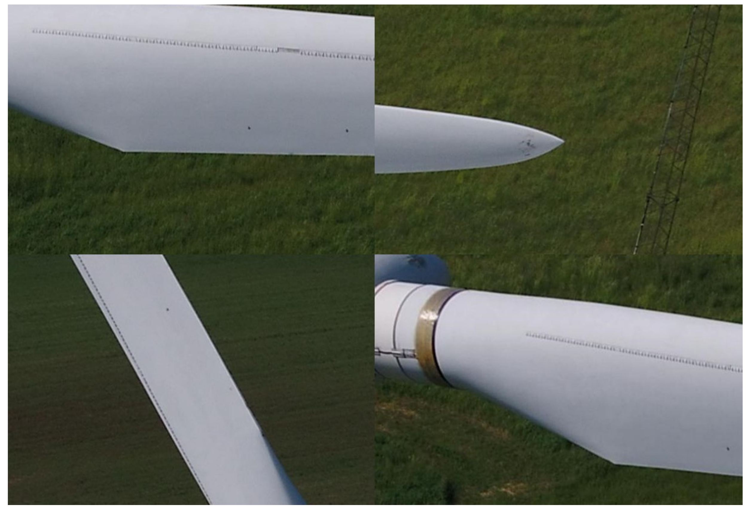
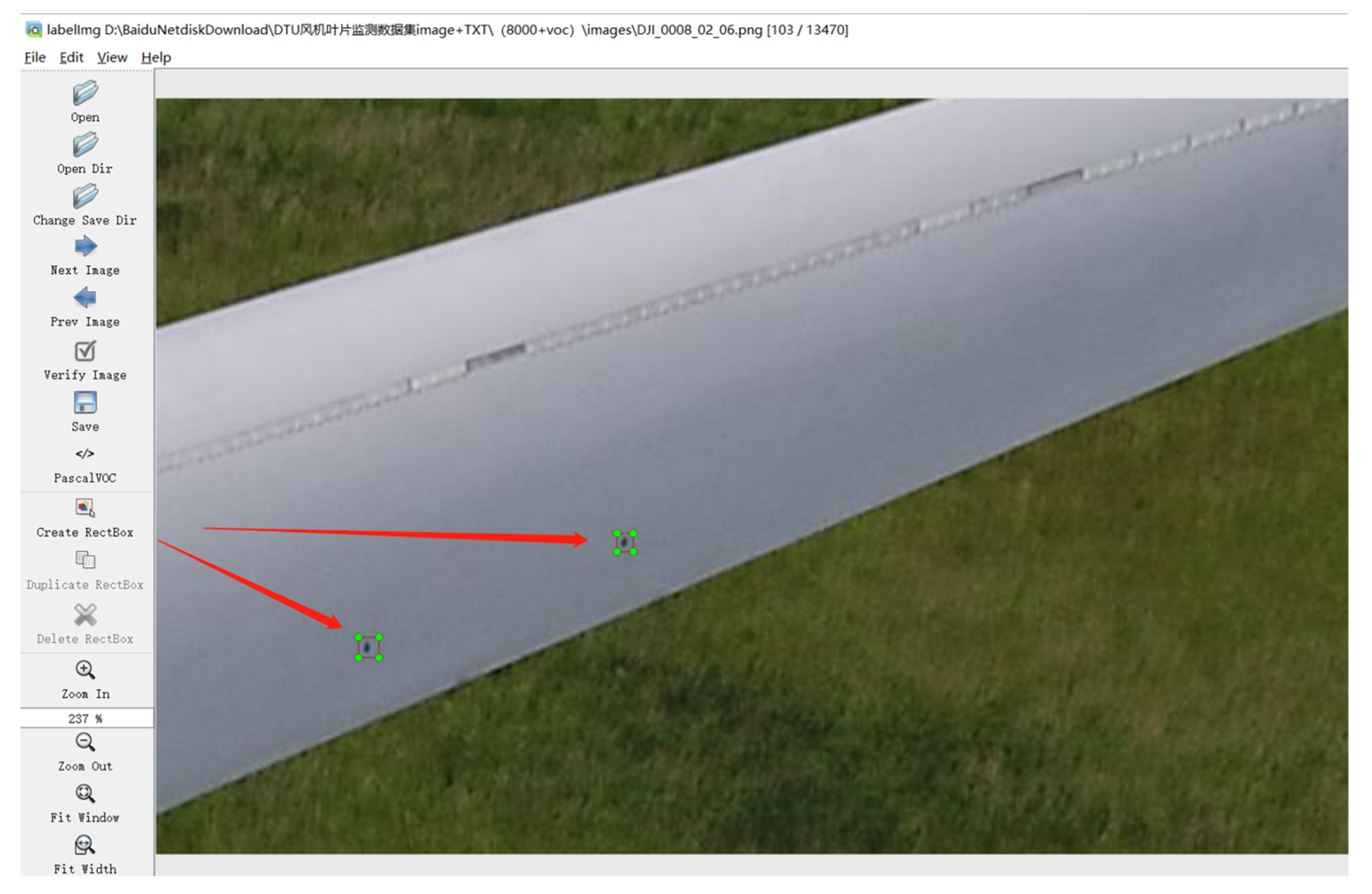
2.1. Dataset Preparation

This article uses the DTU wind turbine unmanned-aerial-vehicle-detecting public dataset. Among them, 2900 high-quality images were selected as the dataset for this experiment and were divided into a training set and a testing set in an 8:2 ratio. Among them, there are 2392 training sets and 598 testing sets. The sample dataset is shown in Figure 3. This article uses the visual image annotation tool LabelImg software 1.3.0 to label oil stains and damage defects in the image and generates defect label information. The interface is shown in Figure 4.

2.2. The Experimental Environment

The experimental environment configuration for this paper’s model is shown in

Table 1. Experimental environment configuration table.

Hardware/System	Model/Version
Operating system	Windows 10
CPU	Intel Core i7-8700
GPU	NVIDIA GeForce RTX 2080Ti 32 GB
Deep Learning Framework	Pytorch 1.13.1
Evelopment language	Python 3.8

.

2.3. Experimental Parameter Setting

The model training in this article enables Mosaic data augmentation, and the SGD optimizer is used to iteratively update the network parameters. The learning rate decay strategy is cosine annealing; Input image size is 640 × 640 × 3. The batch size is set to 32, that is, 32 images are inputted into the network each time, and 300 epochs are trained. The main settings of the hyperparameter are the following: the initial learning rate is 0.001, the momentum is 0.937, the recurrent learning rate Irf is 0.001 and the weight decay coefficient is 0.001.

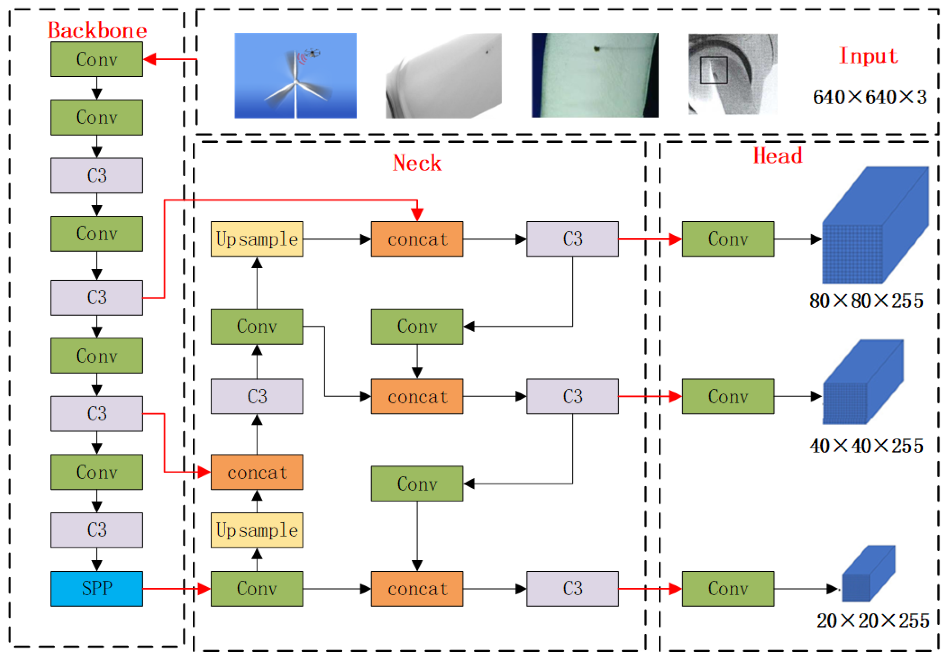
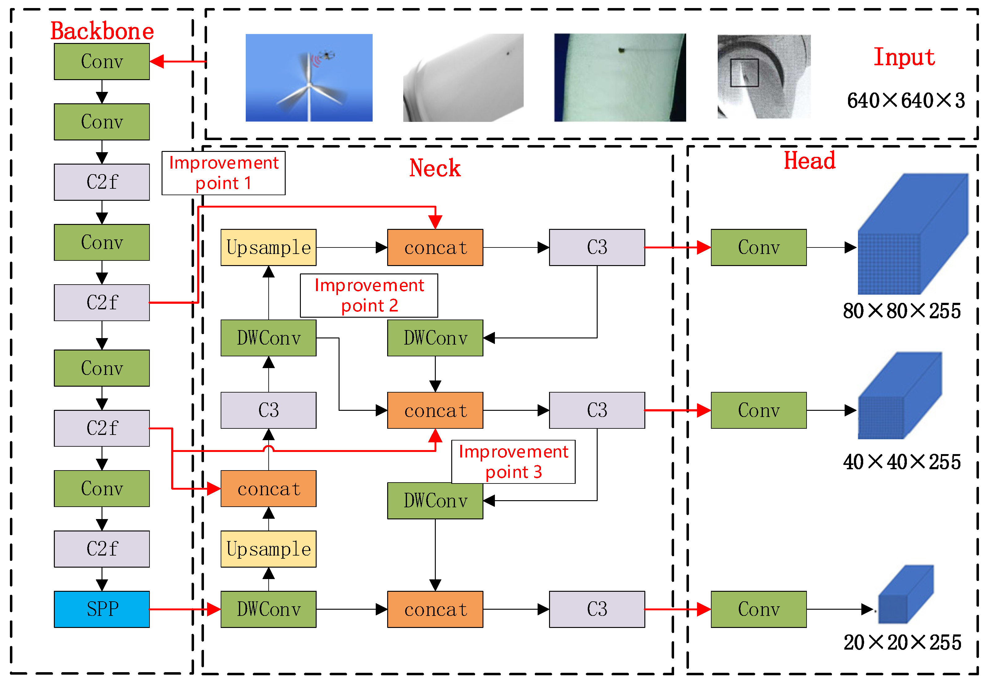
2.4. YOLOv5 Algorithm Improvement

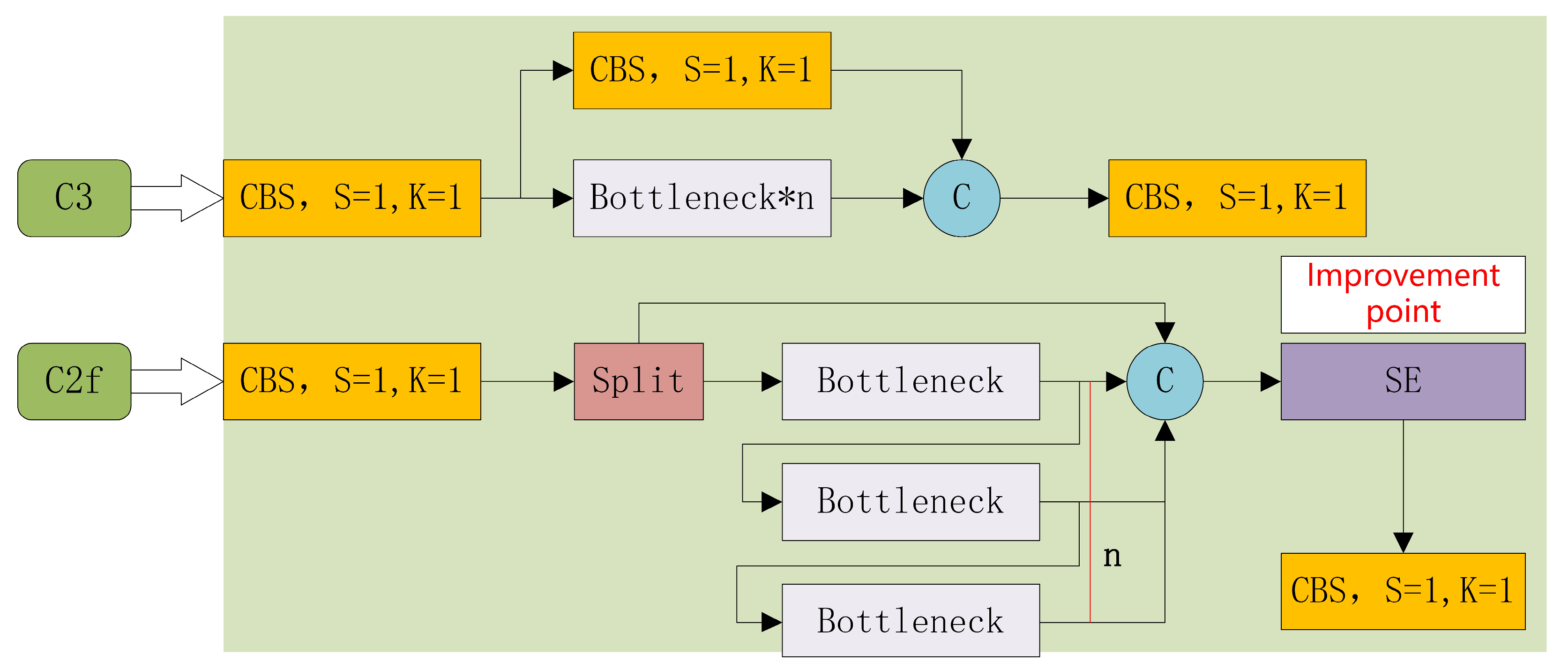
2.4.1. C2f Module Improvement

Because the wind turbine is subjected to complex environmental conditions, its surface is prone to oil pollution, cracks, corrosion and other defects and a large number of early defects that are more difficult to distinguish than general objects and backgrounds. The SE attention mechanism can emphasize more important defect information and suppress redundant feature information such as unimportant backgrounds, especially for small targets, so that the model can locate and identify defect areas more accurately. The C2f module can extract more high-level semantic information while maintaining feature resolution. Therefore, in this essay, we introduce SE attention mechanisms into the Backbone network and embed them into the C2f module to form an improved C2f module to replace the C3 module in Backbone network.

Specifically, the C2f module consists of three branches: one 1 × 1 convolution branch, one 3 × 3 convolution branch and one 5 × 5 convolution branch. The three branches can simultaneously process different-sized receptive fields to extract more comprehensive feature information. In addition, the C2f module also adopts a new progressive down-sampling strategy, which can increase the size of the receptive field while maintaining the resolution of the feature, thus further improving the detection accuracy. The contrast structure between C2f and C3 is shown in Figure 5.

SE-Net is the structure of the network resulting from the fusion of channel attention and spatial attention proposed by Huetal in 2017, as shown in Figure 6, where W, W′, H and H′ are the widths and heights of the feature graph; C and C′ are the number of channels; and FSP is the compression operation, that is, global average pooling. FEX is the incentive operation to reduce the number of channels and thus reduce the amount of computation. Fscale is the multiplication of channel weights, the size of the input feature graph is W′ × H′ × C′, and the size of the final output feature graph is WHC.

As can be seen in Figure 7, the SE module consists mainly of two parts: Squeeze and Excitation, through which the global information is processed [17]. Squeeze: global average pooling of input images yields global statistics for each channel.

$$z_c=F_{sq}\left(u_c\right)=\frac{1}{H\times W}\sum _{i=1}^H \sum _{j=1}^W u_c(i,j)$$

(1)

where represents the global average of the c channel. Excitation: based on the results of Squeeze, the importance of each channel is predicted, and the weighting coefficient of each channel is obtained through Excitation, which is used to weight the characteristic graph of each channel. The mathematical expression is as follows:

s = F_ex(z, W) = σ(g(z, W)) = σ(W₂δ(W₁z))

(2)

Among them, there are two linear transformation matrices, which are activation functions, usually using the ReLU function. s is the channel weight coefficient, with the σ function scaling the weight coefficient between (0, 1).

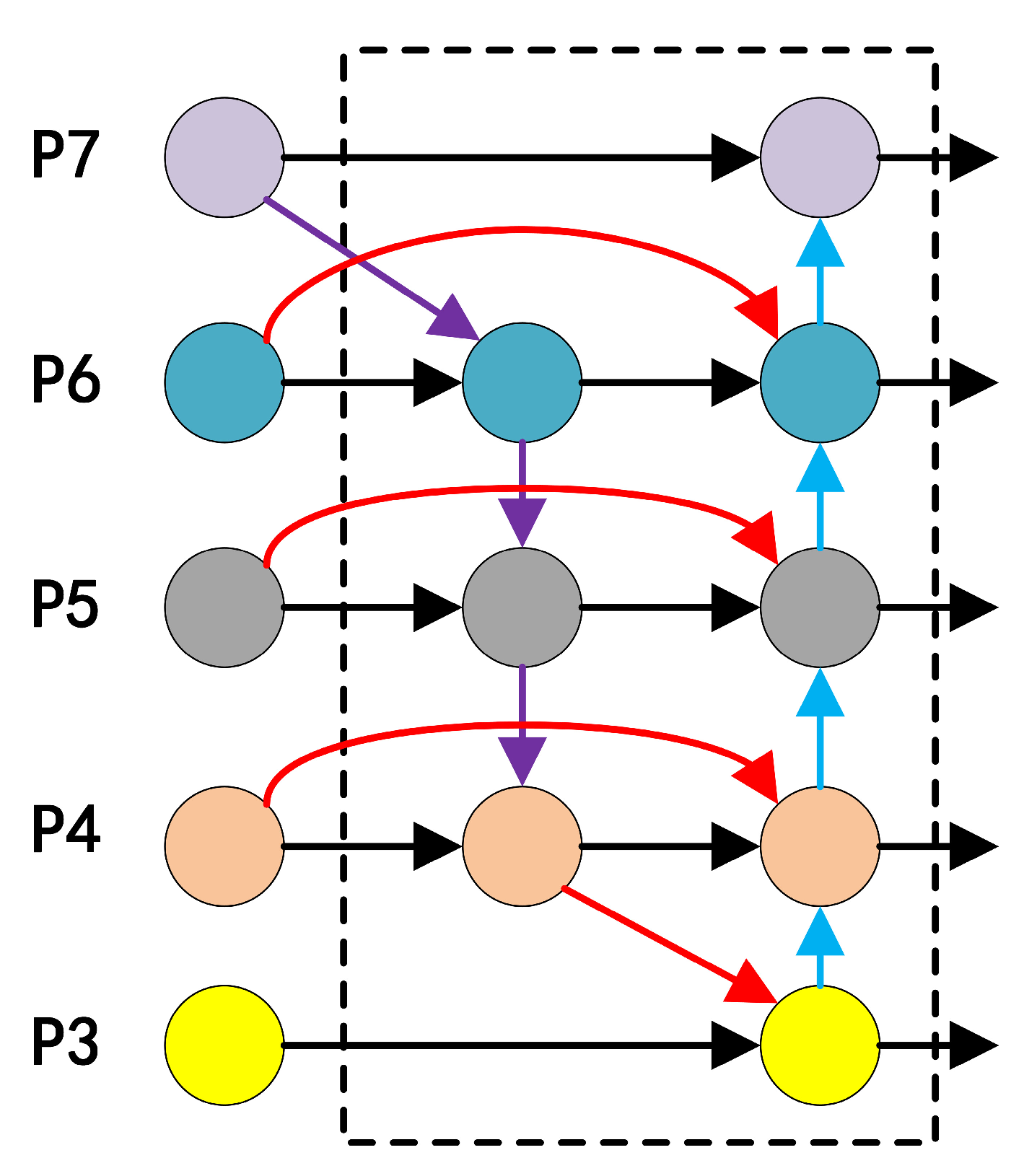
2.4.2. Neck Network Improvement

In the Neck network, on the one hand, we replace the Conv of the Neck network with the DWconv and further seek to reduce the parameters and computation; by convolving each channel of the feature graph, point wise (1 × 1) convolution is used to modify the number of channels, as shown in Figure 8. On the other hand, BiFPN is introduced to replace the Neck network (FPN + PAN) in the original YOLOv5 network to avoid missing detection. In order to simplify the network structure and achieve better feature fusion, BiFPN deletes the nodes with less contribution to feature fusion. Each bidirectional path is treated as a feature network layer, and the same layer is repeated many times. The BiFPN network structure is shown in Figure 9. Two kinds of defect features in a dataset tag are extracted from the Backbone network and are unified and compressed after channel fusion, then the C2f layer and DWconv layer are calculated. Finally, the detection results of small targets on the wind turbine surface are sent out.

2.4.3. Classification Loss Function Improvement

Because there are a lot of background frames as negative samples in the training process, it is often helpful to train a small number of positive samples, resulting in the positive and negative samples to be very unbalanced. In order to solve this problem, the Focal Loss function is introduced to balance positive and negative samples to improve the training efficiency and increase the detection accuracy.

Focal Loss is based on the Binary Cross Entropy Loss function. By adding a dynamic scaling factor, the weight of the easy-to-distinguish samples is dynamically reduced, so that the center of gravity is quickly focused on the hard-to-distinguish samples. The formula is as follows.

On the basis of the Binary Cross Entropy Loss function, the α balance factor is added. By controlling the class weight, the positive and negative samples are balanced, and by adding the (1 − p)^γ modulation factor, the difficult and easy samples are distinguished, increasing the loss proportion of hard-to-distinguish samples.

$$L_{cls}\left(P_{x,y},c_{x,y}^{*}\right)=-\alpha (1-p{)}^{\gamma }{\log }_p(p)$$

(3)

$$p=\left\{\begin{array}{cc}{p}_{x,y},\hfill & \mathrm{if} c_{x,y}^{*}=1\\ 1-p_{x,y},& \mathrm{otherwise}\end{array}\right.$$

(4)

In the above equation, p_x,y represents the classification score predicted by different pixels on the image, and $c_{x,y}^{*}$ represents the category labels corresponding to different pixels on the image.4.

2.5. Evaluating Indicator

In the field of target detection, mean average precision (mAP) is widely used to measure the accuracy of the classification and location of model prediction boxes. Here is a brief introduction to mAP concepts:

Precision = TP/(TP + FP)

(5)

Recall = TP/(TP + FN)

(6)

Among them, TP (True Positive) indicates the number of correctly classified objects detected; FP (False Positive) indicates that the target is detected as an object of another classification. In other words, it is a false detection; FN (False Negative) denotes objects that should be detected but are not, and TN (True Negative) denotes any objects that should not be detected. The curve drawn with the precision of a certain type of defect as the vertical axis and the recall as the horizontal axis is called the P–R curve. The area enclosed by this curve and the horizontal axis is the average accuracy AP of this type of defect. The average accuracy mAP can be obtained by calculating the AP of all types of defects. The calculation formulas are as follows:

$$AP={\int }_0^1 P(R)dR$$

(7)

$$mAP=\frac{\sum _{n=1}^N AP(n)}{N}$$

(8)

3. Results

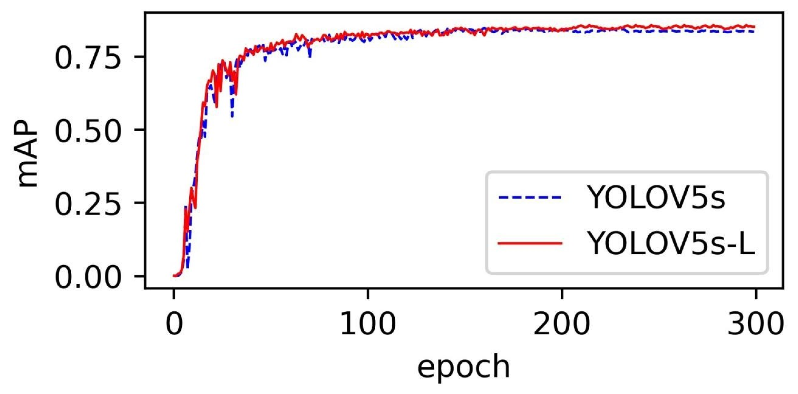
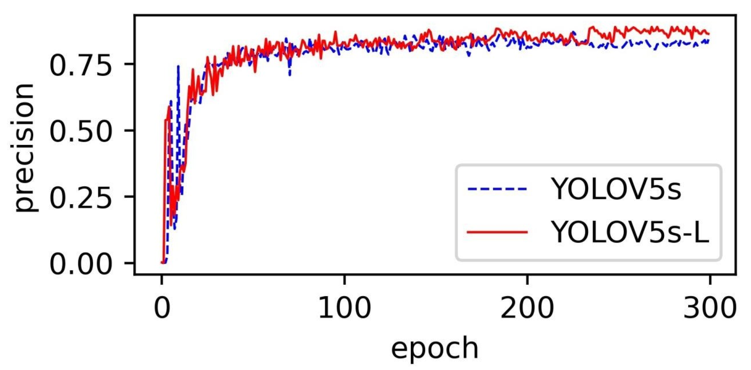
3.1. Comparison of Detection Algorithms

In order to verify the accuracy and validity of the improved algorithm, several models are needed for ablation experiments, which are YOLOv5s-C2f, YOLOv5s-SE, YOLOv5s-BiFPN, YOLOv5s-DW, YOLOv5s-F and YOLOv5s-L. YOLOv5s-C2f replaces the C3 module in the Backbone network with the C2f module. YOLOv5s-SE is the convolutional output layer that embeds the SE attention mechanism into each C2f module and C3 module. YOLOv5s-BiFPN replaces PAN + FPN with BiFPN in the Neck network. YOLOv5s-DW is the replacement of a partial Conv module in the Neck network with a DWconv module. YOLOv5s-F changed the loss function to Focal Loss. YOLOv5s-L is an improved algorithm proposed in this paper.

As shown in

Table 2. Ablation experiments.

Algorithms	C2f	SE	BiFPN	DWconv	Focal-Loss	mAP@0.5	Weight (m)
YOLOv5s-	-	-	-	-	-	0.839	13.7
YOLOv5s-C2f	*	-	-	-	-	0.846	14.9
YOLOv5s-SE	-	*	-	-	-	0.843	13.8
YOLOv5s-BiFPN	-	-	*	-	-	0.842	13.7
YOLOv5s-DW	-	-	-	*	-	0.838	12.2
YOLOv5s-F	-	-	-	-	*	0.841	13.7
YOLOv5s-L	*	*	*	*	*	0.858	13.9

An * indicates that this functionality is available.

, the improved YOLOv5s-L model has higher detection accuracy without adding model parameters. The C2f module and SE attention mechanism increase the parameters of the model but improve the precision of the algorithm greatly. BiFPN and Focal Loss did not increase the weight of the model but improved the precision of the algorithm by a small margin. Although DWconv has a small decrease in accuracy, it greatly reduces the parameters of the model. By combining the above improvements with YOLOv5s, the YOLOv5s-L algorithm can effectively improve the accuracy of the algorithm without increasing the parameters of the control model. Figure 10 shows a mAP@0.5 plot of YOLOv5s-L versus YOLOv5s. You can see that YOLOv5s-L has a distinct advantage over YOLOv5s.

At the same time, this article also selected several mainstream object detection algorithms that are homogeneous with YOLOv5s, mainly including YOLOv5s, SSD and Faster R-CNN algorithms. Under the same dataset, experimental parameters and training strategy, the above object detection algorithms were trained and tested to obtain a comparison table of mAP, detection speed, model size and model complexity for each algorithm’s defect detection.

As shown in

Table 3. Performance comparison before and after model improvement.

Algorithms	mAP@0.5	Weight (m)
Faster R-CNN	0.877	331.1
SSD	0.782	181
YOLOV5s	0.839	13.7
YOLOV5s-L	0.858	13.9

, the two-stage Faster R-CNN algorithm is slightly more accurate because of the traversal of candidate regions and the complexity of the model, but at the same time, it results in too much model weight and a reasoning speed that is too slow, which are not suitable for mobile deployment. Compared with the one-stage algorithm SSD, the improved YOLOv5s has higher precision and is a smaller model, and compared with the one-stage algorithm YOLOv5s, the improved YOLOv5s has higher precision when the parameters are basically the same.

From the experimental results, it can be seen that the improved YOLOv5 model in this article has better overall performance compared to several mainstream algorithms. Compared to the two-stage algorithm Faster R-CNN, although the accuracy decreases by 1.9%, the model size is only 4.1% of it; compared to the first-stage algorithm SSD, it not only leads by 7.6% in average detection accuracy but also has much lower model weights than SSD; and compared to the one-stage algorithm YOLOv5s, the accuracy has been improved by 1.9%, while the model parameters are basically the same. So, the improved YOLOv5s algorithm proposed in this article is more suitable for deployment on mobile devices and low-cost industrial applications.

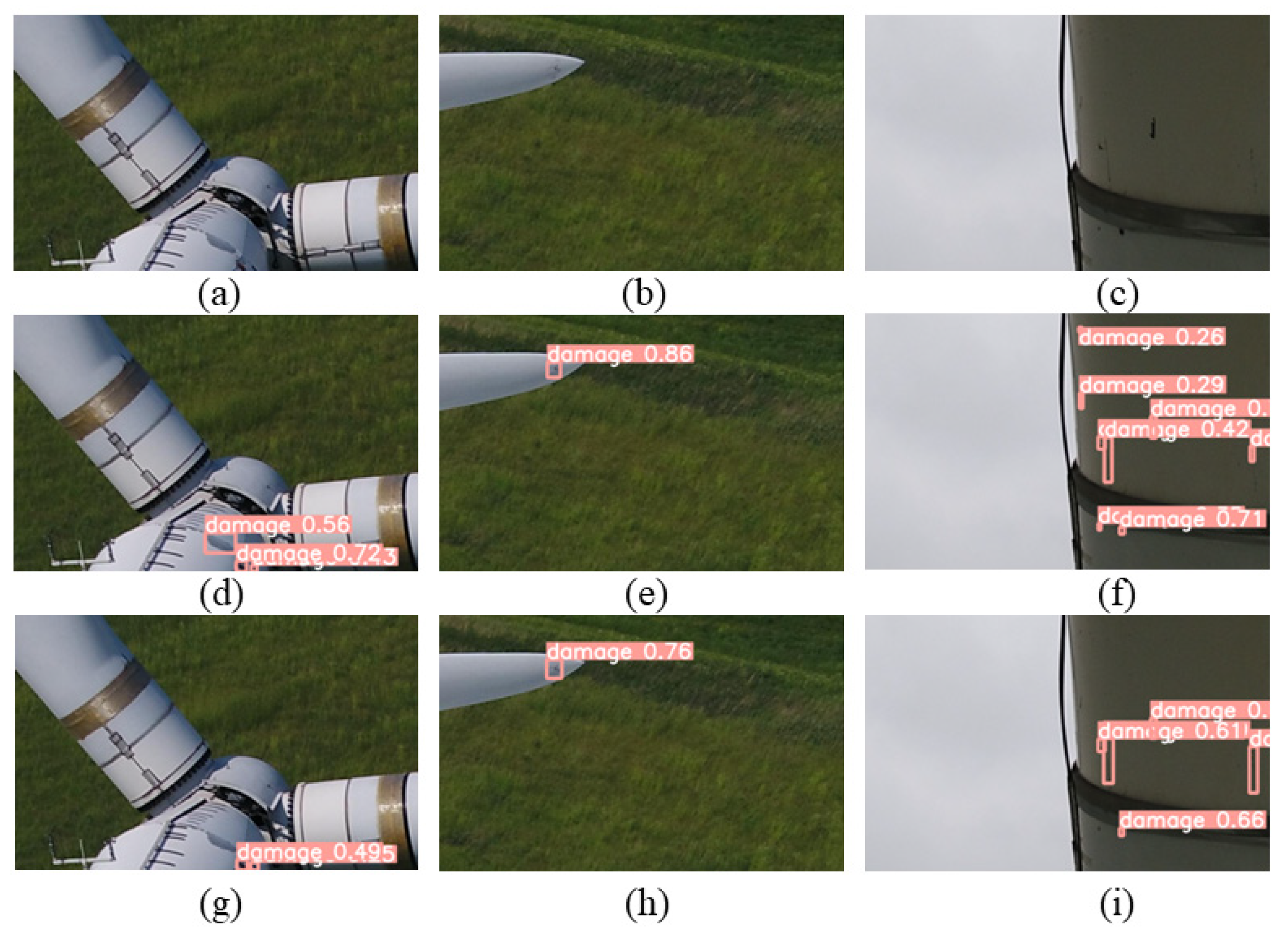
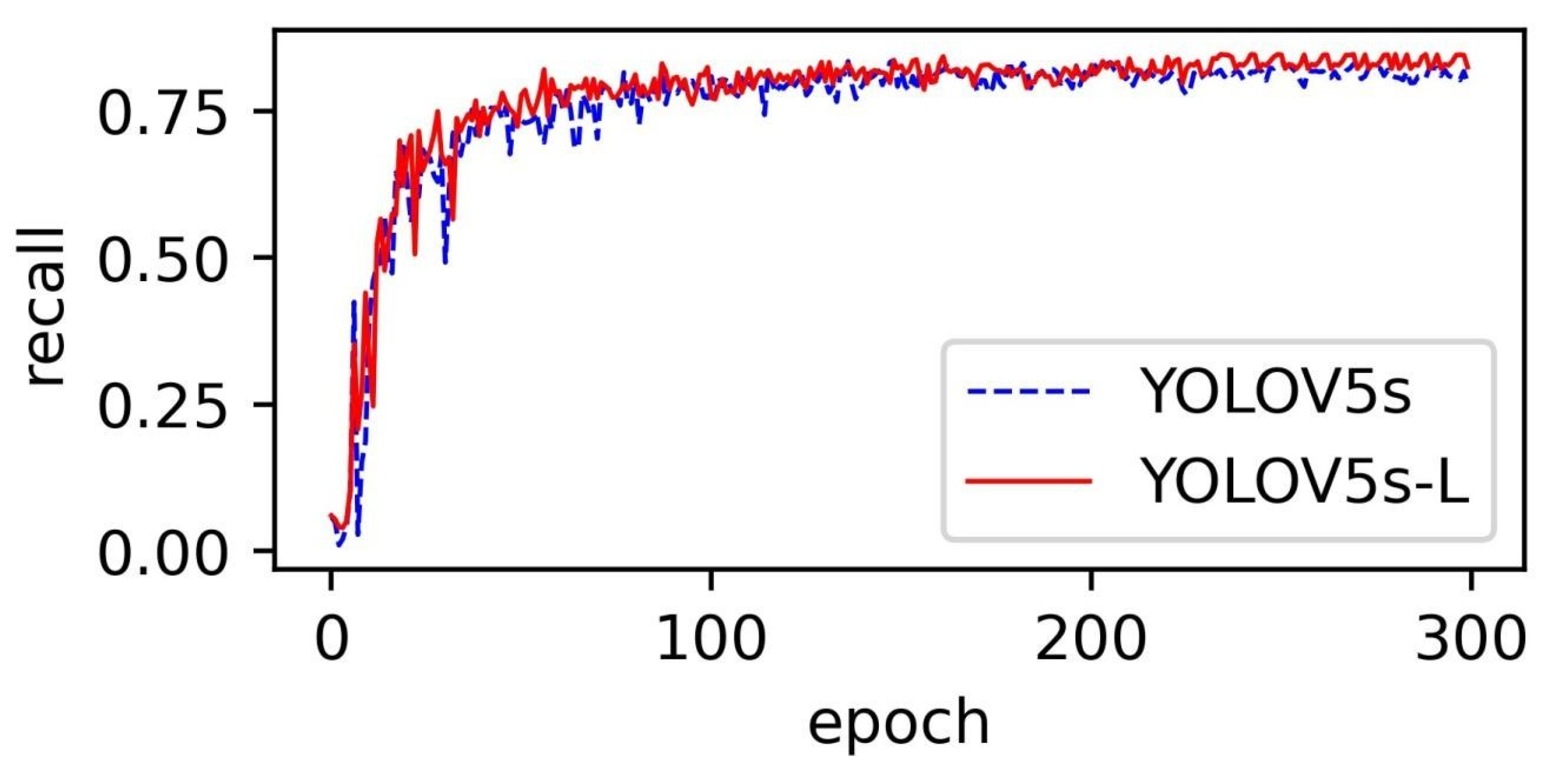
3.2. Contrast Analysis of Detection Effect

In order to verify the effectiveness of the improved YOLOv5 model, the original YOLOv5s model and the improved YOLOv5 model are used to detect wind turbine images. The results are shown in Figure 11.

As shown in Figure 11, the traditional YOLOv5s algorithm has unsatisfactory detection performance. In complex backgrounds, due to insufficient feature extraction and insufficient attention to small targets, there are problems such as missed detection and low accuracy. In the two images g and i, there are many small targets, and there are cases of missed detection for damage. In the h image, the accuracy of dirt detection is not high enough. The YOLOv5s-L algorithm proposed in this article can fully extract image features and focus on small targets by embedding the SE attention mechanism into the C2f module. While improving recall, it can also improve precision. The SE attention mechanism is embedded into the C3 module of the Neck network, and DWconv is used to make the Neck network more lightweight. Finally, BiFP is used for multi-scale feature fusion to increase feature fusion capability. From the precision curve in Figure 12 and the recall curve in Figure 13, it can be seen that compared to the original YOLOv5, mAP increased by 1.9% and recall increased by 1.1%. Therefore, the YOLOv5s-L algorithm can better detect the surface of wind turbines in complex backgrounds.

4. Conclusions

Compared to the traditional YOLOv5 algorithm, our improved YOLOv5 algorithm is more effective in the detection of wind turbines. Therefore, we propose an improved algorithm based on the YOLOv5 model. The main innovations are as follows:

(1)

The introduction of C2f modules to optimize the neural network, increasing the accuracy;

(2)

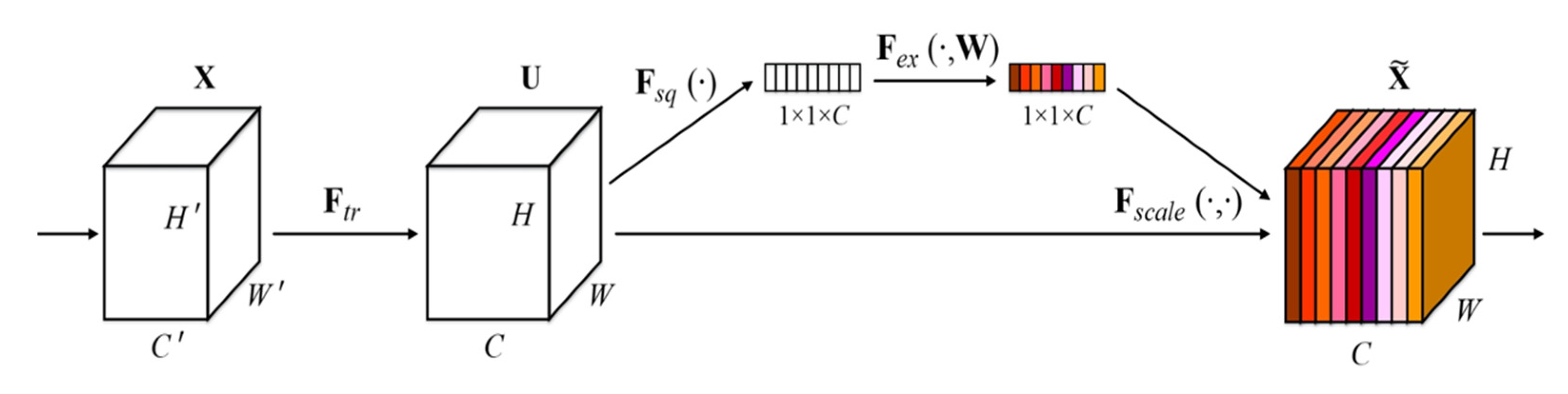
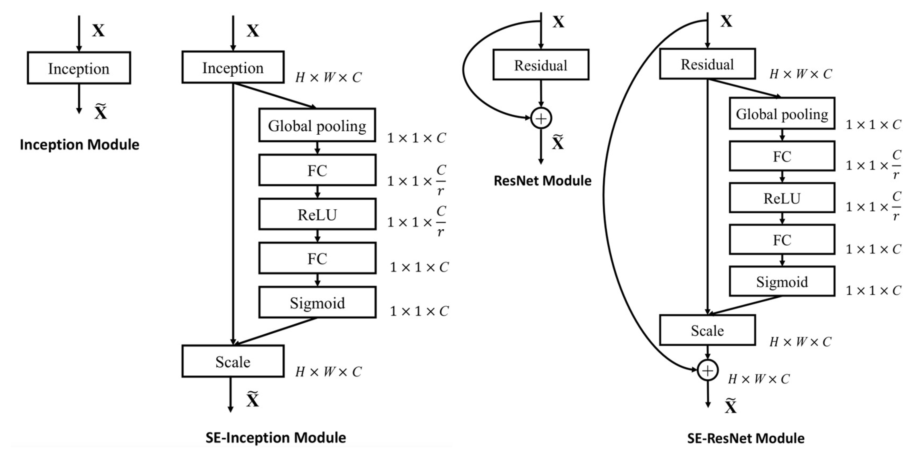
The SE attention mechanism extracts important characteristic information and enhances attention to small targets;

(3)

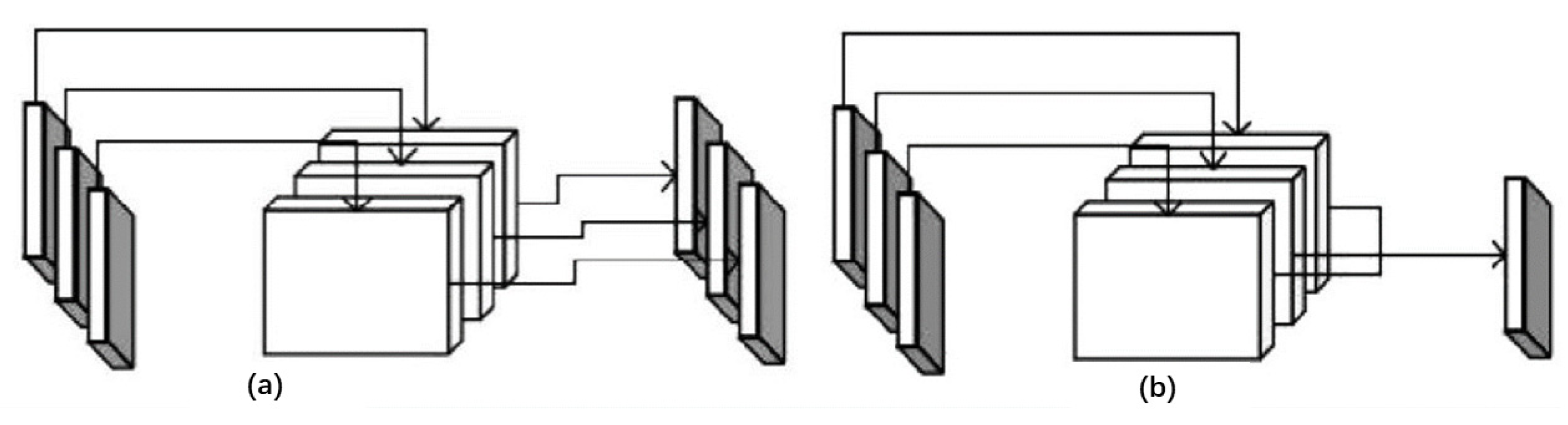
BiFPN is introduced to optimize Neck networks for multi-scale fusion;

(4)

DWconv ensures lightweight network accuracy.

The experimental and detection results show that the improved method in this paper outperforms the original YOLOv5 algorithm in terms of detection accuracy and speed. The optimal weights trained in this paper are validated, and compared with the original YOLOv5, the mAP increases by 1.9% with almost the same parameter quantity. The overall performance is high, providing support for the automatic analysis of wind turbine image detection and achieving low-cost inspection of surface defects.

References

1. Hsu, J.Y.; Wang, Y.F.; Lin, K.C. Wind turbine fault diagnosis and predictive maintenance through statistical process control and machine learning. IEEE Access 2020, 8, 23427–23439. [Google Scholar] [CrossRef]
2. Wang, L.; Zhang, Z.; Long, H.; Xu, J.; Liu, R. Wind Turbine Gearbox Failure Identification With Deep Neural Networks. IEEE Trans. Ind. Inform. 2017, 13, 1360–1368. [Google Scholar] [CrossRef]
3. Wang, L.; Long, H.; Zhang, Z.; Xu, J.; Liu, R. Wind turbine gearbox failure monitoring based on SCADA data analysis. In Proceedings of the 2016 IEEE Power and Energy Society General Meeting (PESGM), Boston, MA, USA, 17–21 July 2016; IEEE: Piscataway, NJ, USA, 2016; pp. 1–5. [Google Scholar]
4. Long, H.; Wang, L.; Zhang, Z.; Song, Z.; Xu, J. Data-driven wind turbine power generation performance monitoring. IEEE Trans. Ind. Electron. 2015, 62, 6627–6635. [Google Scholar] [CrossRef]
5. Ruiz, M.; Mujica, L.E.; Alferez, S.; Acho, L.; Tutiven, C.; Vidal, Y.; Rodellar, J.; Pozo, F. Wind turbine fault detection and classification by means of image texture analysis. Mech. Syst. Signal Process. 2018, 107, 149–167. [Google Scholar] [CrossRef]
6. Zhuang, Y.; Ruan, C.; Qiu, K.; Xu, H. Comparison of non-destructive testing methods for fan blade defects. Technol. Innov. 2016, 57, 106. [Google Scholar]
7. David, G.; Dmitri, T. An experimental study on the data-driven structural health monitoring of large wind turbine blades using a single accelerometer and actuator. Mech. Syst. Signal Process. 2019, 127, 102–119. [Google Scholar]
8. Munteanu, E.; Zaporojan, S.; Dulgheru, V. Intelligent Condition Monitoring of Wind Turbine Blades: A Preliminary Approach. In Proceedings of the 2022 IEEE 18th International Conference on Intelligent Computer Communication and Processing (ICCP), Cluj-Napoca, Romania, 22–24 September 2022; pp. 9–16. [Google Scholar]
9. Worzewski, T.; Krankenhagen, R.; Doroshtnasir, M. Thermographic inspection of wind turbine rotor blade segment utili-zing natural conditions as excitation source, Part Il;The effectof climatic conditions on thermographic inspections-A longterm outdoor experiment. Infrared Physics. Technology 2016, 76, 767–776. [Google Scholar]
10. Li, J.; Ye, D.H.; Chung, T. Multi-target detection and tracking from a single camera in Unmanned Aerial Vehicles (UAVs). In Proceedings of the 2016 IEEE/RSJ International Conference on Intelligent Robots and Systems (IROS), Daejeon, Republic of Korea, 9–14 October 2016; IEEE: Piscataway, NJ, USA, 2016; pp. 4992–4997. [Google Scholar]
11. Wang, L.; Zhang, Z.; Luo, X. A two-stage data-driven approach for image-based wind turbine blade crack inspections. IEEE/ASME Trans. Mechatron. 2019, 24, 1271–1281. [Google Scholar] [CrossRef]
12. Neupane, D.; Seok, J. A review on deep learning-based approaches for automatic sonar target recognition. Electronics 2020, 9, 1972. [Google Scholar] [CrossRef]
13. Jiang, P.; Ergu, D.; Liu, F.; Cai, Y.; Ma, B. A Review of Yolo algorithm developments. Procedia Comput. Sci. 2022, 199, 1066–1073. [Google Scholar] [CrossRef]
14. Wang, G.; Chen, S.; Hu, G.; Pang, D.; Wang, Z. Detection algorithm of abnormal flow state fluid on closed vibrating screen based on improved YOLOv5. Eng. Appl. Artif. Intell. 2023, 123, 106272. [Google Scholar] [CrossRef]
15. Yu, Y.; Zhao, J.; Gong, Q.; Huang, C.; Zheng, G.; Ma, J. Real-time underwater maritime object detection in side-scan sonar images based on transformer-YOLOv5. Remote Sens. 2021, 13, 3555. [Google Scholar] [CrossRef]
16. Shihavuddin, A.S.M.; Chen, X.; Fedorov, V.; Nymark Christensen, A.; Andre Brogaard Riis, N.; Branner, K.; Dahl, A.B.; Reinhold Paulsen, R. Wind turbine surface damage detection by deep learning aided drone inspection analysis. Energies 2019, 12, 676. [Google Scholar] [CrossRef]
17. Hu, J.; Shen, L.; Sun, G. Squeeze-and-excitation networks. In Proceedings of the IEEE Conference on Computer Vision and Pattern Recognition, Salt Lake City, UT, USA, 18–23 June 2018; pp. 7132–7141. [Google Scholar]
Figure 1. YOLOv5 network structure.
Ndt 01 00005 g001
Figure 2. Improved YOLOv5 network structure.
Ndt 01 00005 g002
Figure 3. Partial sample dataset.
Ndt 01 00005 g003
Figure 4. An example of defect tagging.
Ndt 01 00005 g004
Figure 5. C2f versus C3.
Ndt 01 00005 g005
Figure 6. SE (Squeeze-and-Excitation) module algorithm flow.
Ndt 01 00005 g006
Figure 7. SE-inception (left) and SE-ResNet (right) modules.
Ndt 01 00005 g007
Figure 8. The depth separable convolution implementation steps. (a) Deep convolution. (b) Point-by-point convolution.
Ndt 01 00005 g008
Figure 9. BiFPN structure.
Ndt 01 00005 g009
Figure 10. Comparison of the mAP between the YOLOv5s and YOLOv5s-L, where the YOLOv5s is the blue curve and the YOLOv5s-L is the red curve.
Ndt 01 00005 g010
Figure 11. Results of two model checks. (ac) are the original images of YOLOv5s detection effects, (df) are the YOLOv5s-L detection effects, and (gi) are the YOLOv5 detection effects.
Ndt 01 00005 g011
Figure 12. Comparison of the precision between the YOLOv5s and YOLOv5s-L, where the YOLOv5s is the blue curve and the YOLOv5s-L is the red curve.
Ndt 01 00005 g012
Figure 13. Comparison of the recall between the YOLOv5s and YOLOv5s-L, where the YOLOv5s is the blue curve and the YOLOv5s-L is the red curve.
Ndt 01 00005 g013