A Novel Method for Reducing the Lift-Off Effect in Coercivity Measurement through Auxiliary Inductance Data

Abstract

Coercivity is the strength of the reverse magnetic field required to demagnetize a material after saturation, and it is an indication of the hardness of magnetic materials. Air gaps cause errors in coercivity measurement referred to as the lift-off effect. This paper proposes a new method to address this issue by incorporating additional inductance measurements and formulating a calibration method. The calibration principle is based on the fact that both the coercivity and the inductance measurements change with the variation of air gaps. This paper starts by finding how coercivity changes with air gaps between the sensor and the sample, then derives the coefficients for the coercivity–inductance relationship for different samples. A correction method is then proposed to predict the base coercivity (i.e., the coercivity when the air gap = 0) using the inductance and coercivity measurement results at an unknown lift-off. The measurement system was implemented, and experimental results suggest the error caused by air gaps can be reduced from 40% to less than 10%.

1. Introduction

Coercivity measurements are widely used in industrial applications owing to their ability to reflect the property and structural integrity of materials. A number of different studies have been carried out to show that coercivity is sensitive to changes in the microstructures of materials and could be used to indicate damage or creep inside materials [1,2,3]. It has been reported that the coercivity of stainless steel follows the tendency of Vickers hardness and reflects the changes in mechanical properties that appear after the quenching process [4]. Mitra et al. [5] correlated the magnetic properties of high-carbon steel, including coercivity and remanence, in the three different creep stages, making it a possible technique for the non-destructive evaluation of internal damage. Based on studies of creep stages, Qi et al. [6] proposed that coercivity can be used to reflect the damage caused by high temperatures and estimate the remaining life of the alloy.

However, it has been observed that the precision and accuracy of coercivity measurement results suffer from the presence of air gaps between the probe and the test samples (lift-off problem) [7]. This effect is considered a critical limitation of the coercivity measurement technique. The contact problem may arise due to rough contact surfaces, insulation shields, or non-standard operations. The variation in the gap has a significant impact on both magnetization and demagnetization processes [8]. Additionally, the effects of electromagnetic noise need to be considered to accurately determine the zero magnetization state [9]. There are a significant number of studies that aim to eliminate or reduce the impact of lift-off. These studies can be mainly divided into two groups: the first aims to reduce the sensitivity of the measuring probe to air gaps [10], whereas the second takes into account the lift-off effect on the measurement results [11].

This paper aims to reduce the lift-off effect on measurement results. It is advisable to consider parameters that are highly sensitive to air-gap variations during data processing, such as magnetic induction and magnetic reluctance [12,13]. Traditional coercivity measurement requires the sensor to be in close contact with the sample. However, in industrial measurements, the sample is always protected by the insulation shield, and removing and reinstalling the insulation shells is costly. Therefore, it would be much simpler to measure the inductances due to the air gap using a specifically designed probe. The purpose of this paper is to develop a model to predict coercivity by performing a single measurement of coercivity and inductance with an air gap between the sample and the sensor (i.e., with lift-off).

Focusing on the relationship between the measured coercivity and the mutual inductance of the entire magnetic loop when lift-off is present (open-loop measurement), the actual coercivity measurement of the sample can be inferred from the measurement result with the air gap. Starting with the measurement of the variation tendency of coercivity and inductances with increasing air gaps for given samples, the relationship between mutual inductances and coercivity is revealed. Extending this relationship to other samples, the curve can be used to identify the base coercivity of the sample from a single coercivity measurement at a random air gap (0–15 mm).

2. Coercivity Measurements Based on Pulse Excitation

2.1. Principle and Components

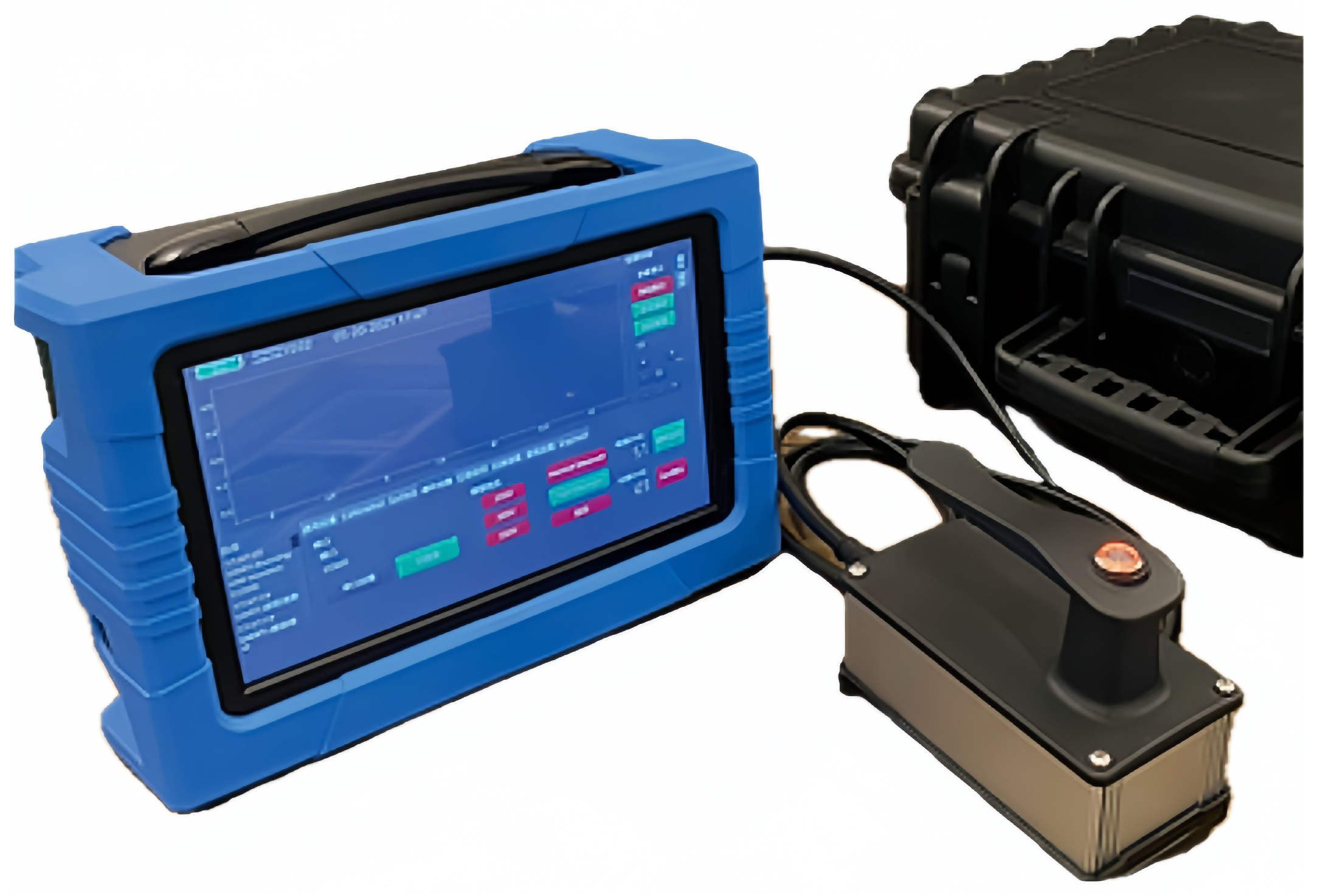
Coercivity refers to the strength of the reverse magnetic field required to demagnetize the sample to zero after it has been magnetized to saturation. This paper is based on a coercivity meter designed by the EM sensing group at the University of Manchester. The coercivity meter is composed of a main instrument and a measurement probe, as shown in Figure 1.

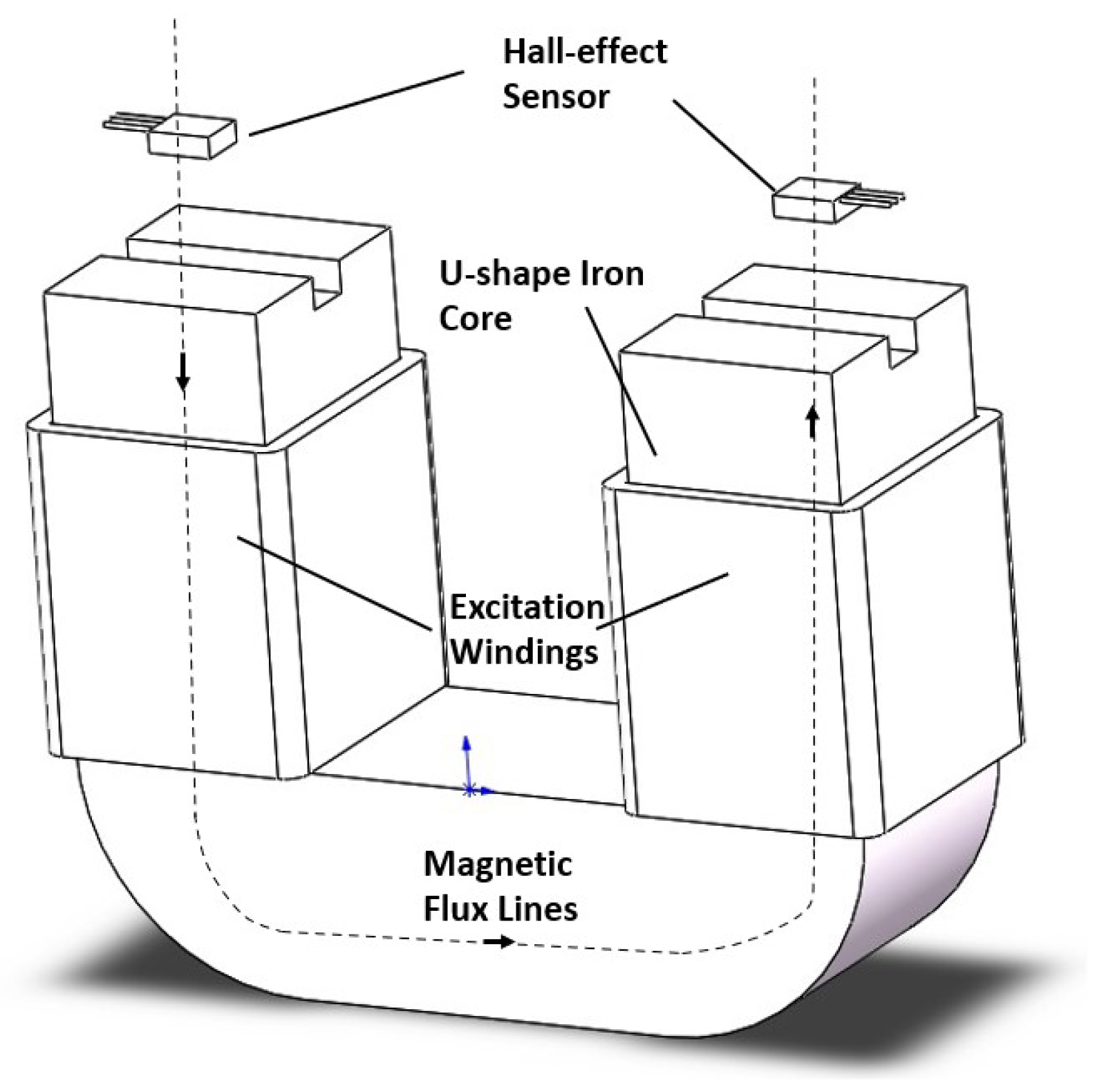
Figure 2 shows the internal structure of the sensor probe, which is composed of a U-shaped iron core, excitation windings, and Hall-effect sensors. With a 64 mm limb and 25 mm thickness, the U-shaped iron core provides a path for the magnetic flux, thereby significantly reducing flux leakage. Excitation windings aim to generate a magnetic field to magnetize the sample under testing to the saturation point. There are many magnetic sensors designed to measure the magnetic properties of the target sample [14,15]. Hall-effect sensors are ratiometric sensors that support large operating bands (10–1000 Gauss) [14,15,16] and are suitable for reflecting changes in the magnitude and direction of magnetic fields. The Hall-effect sensors are mounted at the tip of each limb and are in close contact with both the iron yoke and the surface of the material under testing. The strength of the magnetic field exerted on the sample is related to the magnitude of the current passing through the sensor.

2.2. System Description

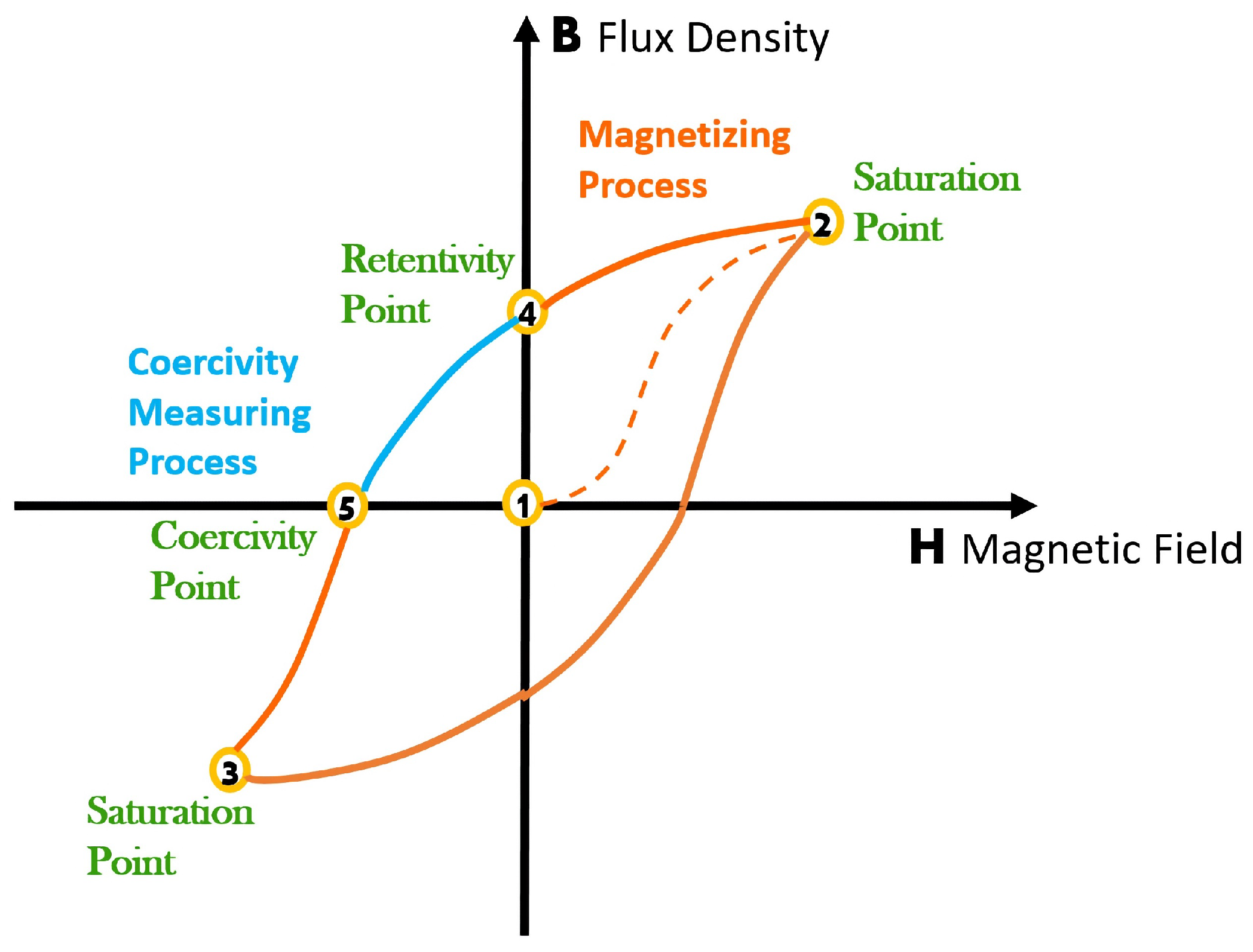
Figure 3 depicts the magnetizing process and the position of the magnetizing stage during the measurement process. The entire measurement process can be divided into the magnetizing process and the coercivity measuring process. During the magnetizing process, the tested samples are subjected to the hysteresis loop.

The measurement process starts by triggering the high-voltage excitation module and conducting high-level voltage up to 350 V to the excitation winding, causing a pulse excitation that magnetizes the sample to reach saturation point 2. As the voltage output of Hall sensors reaches its maximum value, the excitation module is turned off, and the demagnetizing module is sequentially activated. The demagnetizing current applies an opposite polarity magnetic field to the sample, demagnetizing it to saturation point 3. The whole process takes 3.5 s, and it is applicable to all materials. Once the pulse excitation current is switched off, the external applied magnetic field returns to zero, causing the tested sample to return to retentivity point 4. After the magnetizing process is complete, the coercivity measuring process begins.

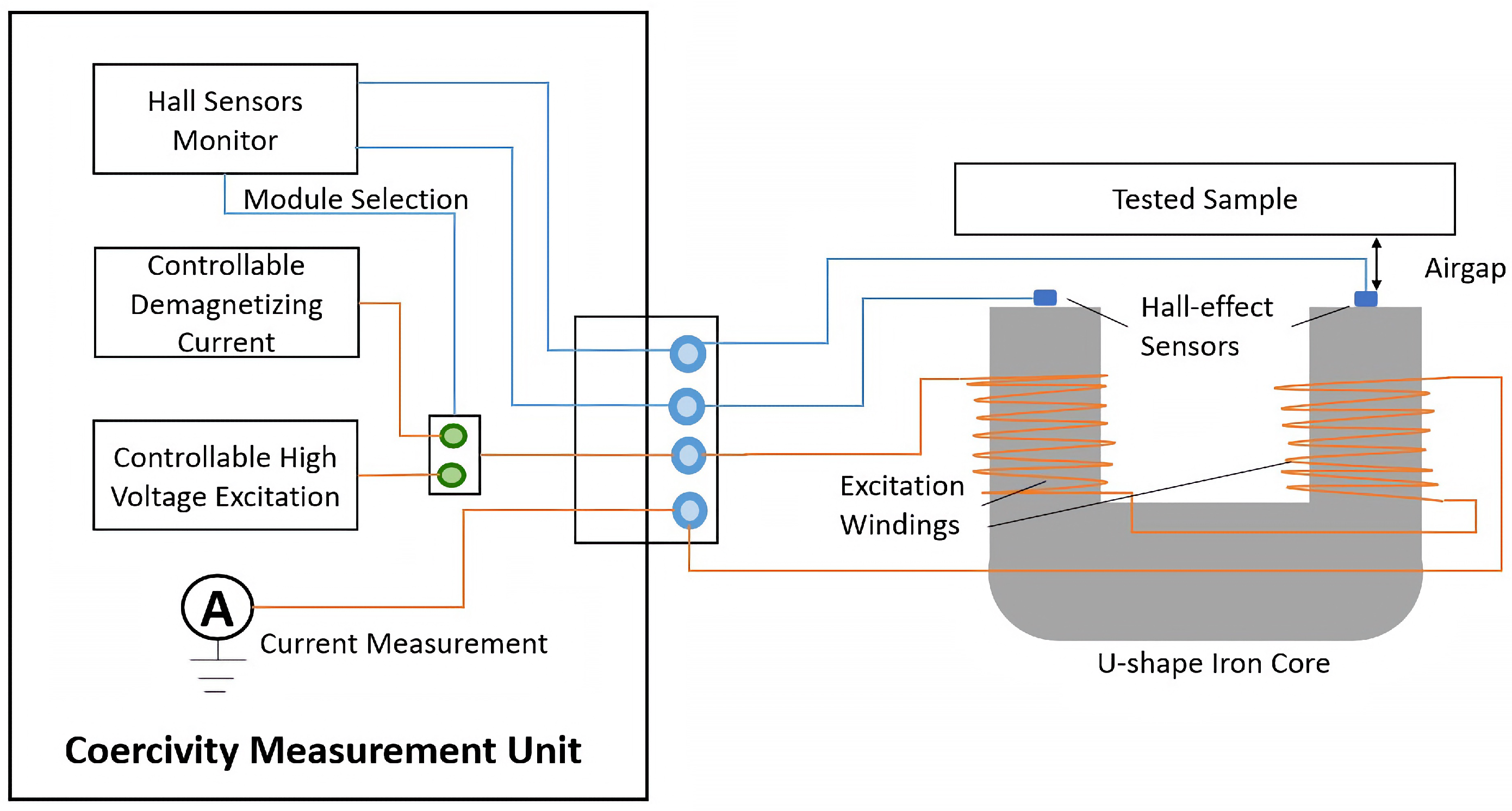
The coercivity measuring process aims to magnetize samples to a coercivity point and subsequently measures the current passing through the winding to determine the coercivity. During the measuring process, the material is forced to oscillate in close proximity to the coercivity point, switching between magnetizing and demagnetizing modes and essentially moving around a very small minor loop. This is implemented by applying a DC-biased small AC current to the excitation winding based on Hall sensor feedback. The sensor output remains non-zero until the sample reaches the coercivity point. The non-zero output will be sent to the Hall sensor monitor and used to select the module conducted to the windings, as shown in the internal structure in Figure 4. Once the output difference becomes zero at the coercivity point, the coercivity is inferred from the DC component of the current flowing through the windings.

3. Methodology

3.1. Inductance Measurement

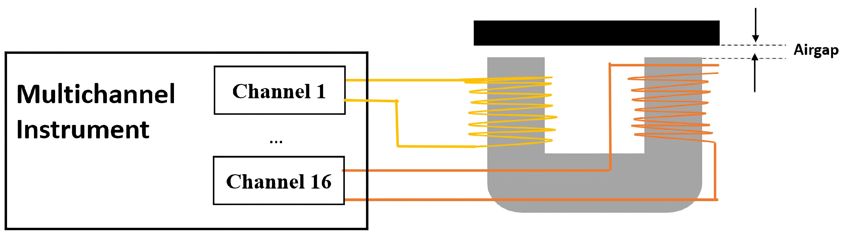
The inductance of the given sample with increasing air gaps is measured using a multichannel instrument with a designed sensor. The measurement is achieved by sequentially selecting the coil pairs, and each channel can be used as an EM excitation source, detection, or both. The instrument is capable of 16 channels multiplexing excitation and receiving synchronized signals during the measurement process.

The sensor is constructed of a U-shaped magnetic yoke and two identical windings. The yellow winding provides excitation, whereas the orange winding measures voltage. In this way, channel 1 and channel 16 are selected as the excitation and receiving channels. The multichannel instrument is employed to measure the inductance of the measurement loop consisting of the probe, air gap, and the tested sample at 1 kHz, 200 kHz, and 500 kHz. The measurement setup is shown in Figure 5.

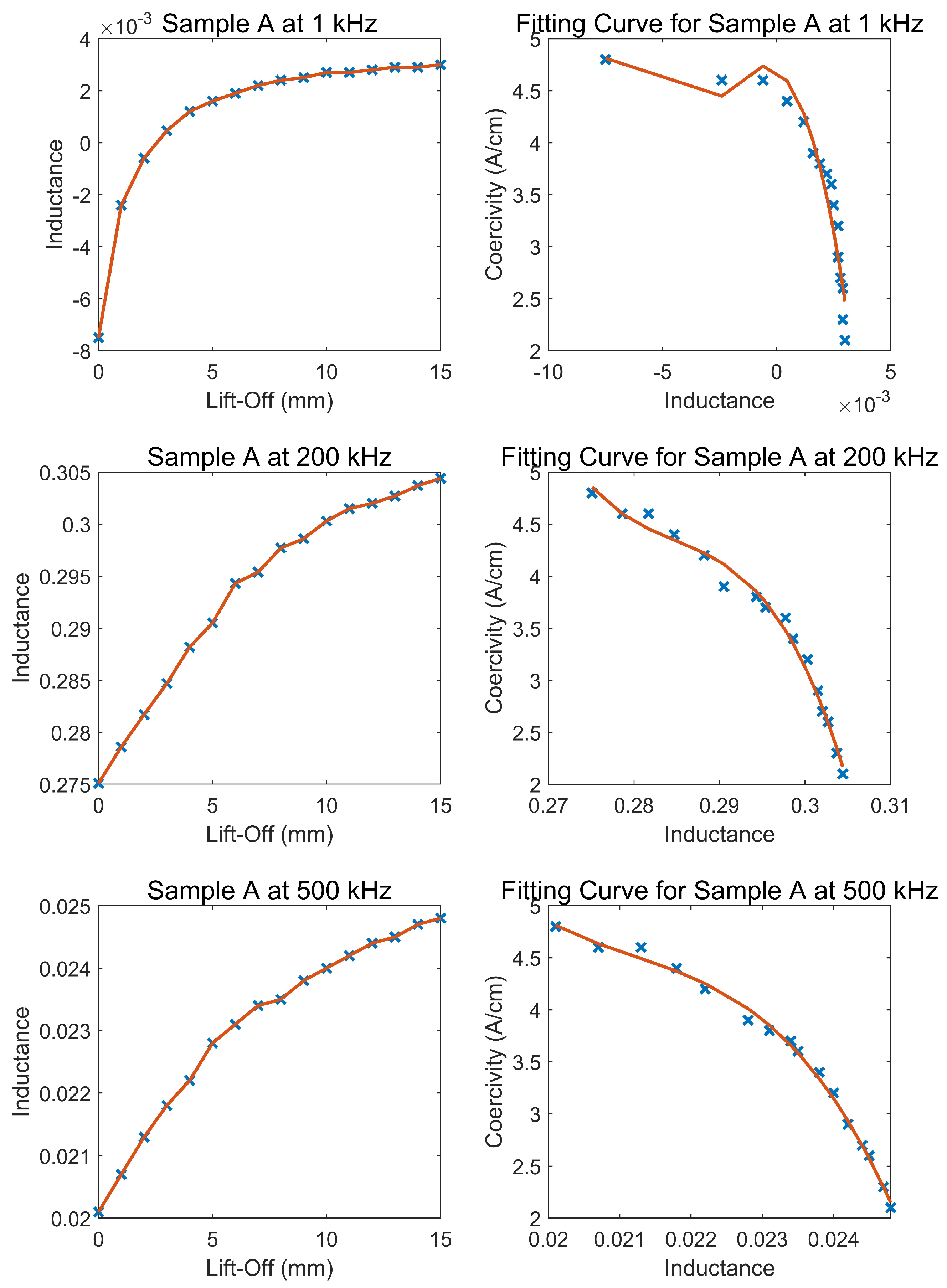
When comparing the measurement results at 1 kHz, 200 kHz, and 500 kHz, it was observed that there was a significant fluctuation in the inductance measured at 1 kHz. To minimize the measurement error, the mean measured inductance for sample A (coercivity equal to 4.8 A/cm) was calculated and is shown on the right side of Figure 6. As for 200 kHz and 500 kHz, the measured inductance for a single lift-off remained at a relatively stable level. Moreover, the inductances for different lift-offs exhibited noticeable distinctions at 200 and 500 kHz. To further determine the most suitable frequency, the measured inductance was used to plot the three-order polynomial curve, as explained in Section 3.2, it is evident that the inductance measured at 500 kHz offers a more precise fit. The goodness of the fitness curve of different frequencies are listed in

Table 1. Goodness of fit for Figure 6.

Fit Curve	1 kHz	200 kHz	500 kHz
Sum-of-squares error	0.0418	0.0078	0.0028
Root-mean-square error (RMSE)	0.0511	0.0220	0.0132

. One possible reason for this observation is that the inductance measurements conducted in the lower frequency range are more sensitive to EM properties associated with the material composition of the U-shaped core and the sample under testing [17].

3.2. Relationship Extrapolation

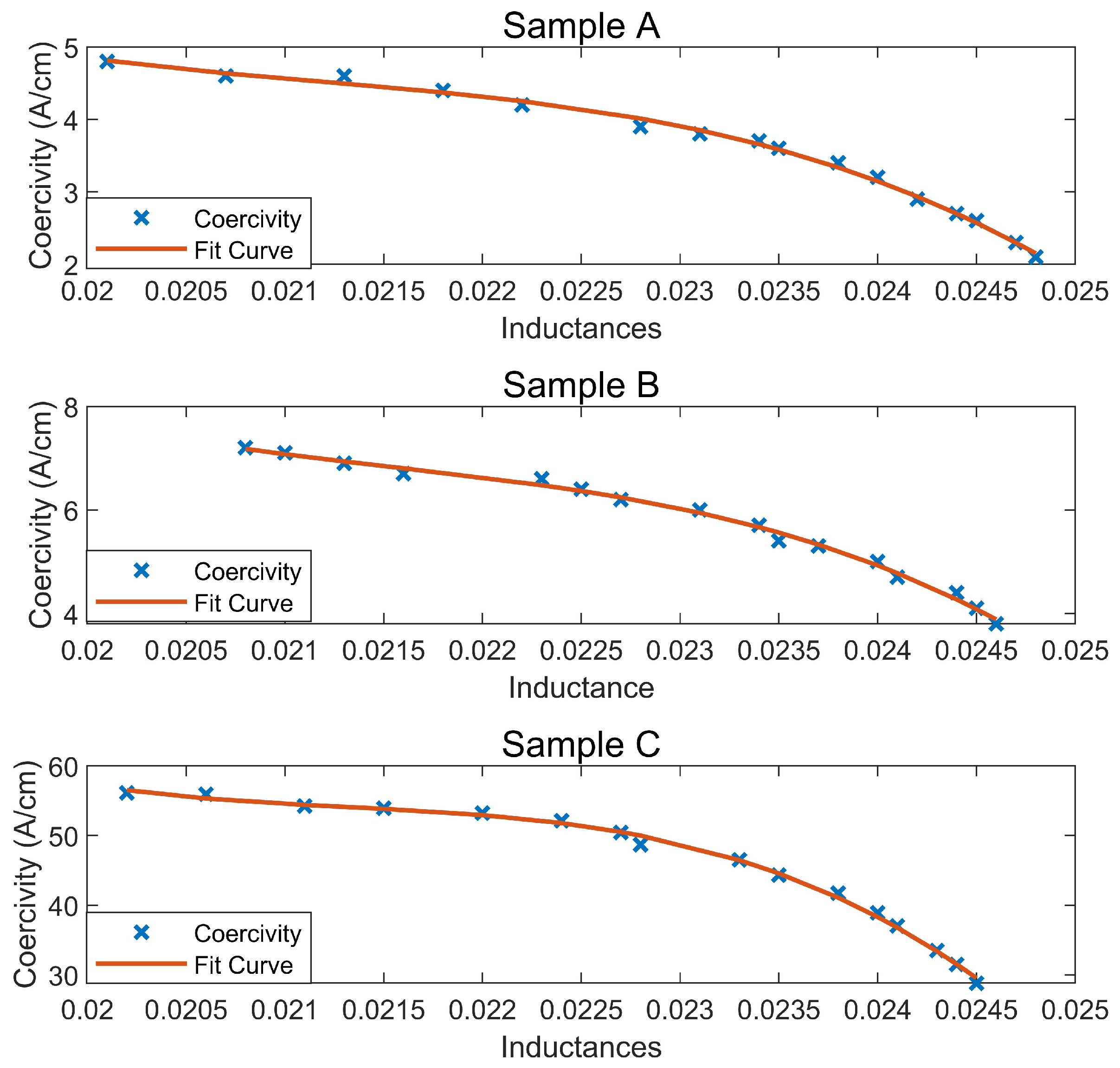
Samples A and B are high-carbon steels, with a carbon composition of 0.6–0.8%. Sample C is A2 tool steel, with a carbon composition of around 0.95%. The coercivity measurements were taken across a range of lift-offs from 0 to 15 mm using the coercivity meter mentioned in Section 2.1. The sizes and coercivities of the samples are shown in

Table 2. Sizes and coercivities of the tested samples.

Test Sample	Sample A	Sample B	Sample C
Coercivity (A/cm)	4.8	7.2	56.0
Size (mm × mm × mm)	80 × 25 × 8	81 × 25 × 8	81 × 27 × 8

.

The three-order polynomial curve is the most suitable fitting curve for all three samples, as indicated by the red lines in Figure 7. The fitting precision is acceptable and the goodness of fitness curves are listed in

Table 3. Goodness of fit for Figure 7.

Fit Curve	Sample A	Sample B	Sample C
Sum-of-squares error	0.0028	0.0061	0.2383
Root-mean-square error (RMSE)	0.0132	0.0195	0.1220

. The functional representation of the inductance–coercivity fitting curve is expressed using Equation (1):

$$H_C^m=a{L}^3+b{L}^2+cL+d$$

(1)

where $H_C^m$ represents the measured coercivity with lift-off; L represents inductances for different air gaps; and a, b, c, and d are constant coefficients. The coefficients of samples A, B, and C are listed in

Table 4. Coefficients for samples A, B, and C.

Coefficients	a	b	c	d
Sample A	−3.268 × 10${}^7$	2.077 × 10${}^6$	−4.425 × 10${}^4$	3.203 × 10${}^2$
Sample B	−5.857 × 10${}^7$	3.792 × 10${}^6$	−8.226 × 10${}^4$	6.048 × 10${}^2$
Sample C	−6.171 × 10${}^8$	3.948 × 10${}^7$	−8.433 × 10${}^5$	6.069 × 10${}^3$

.

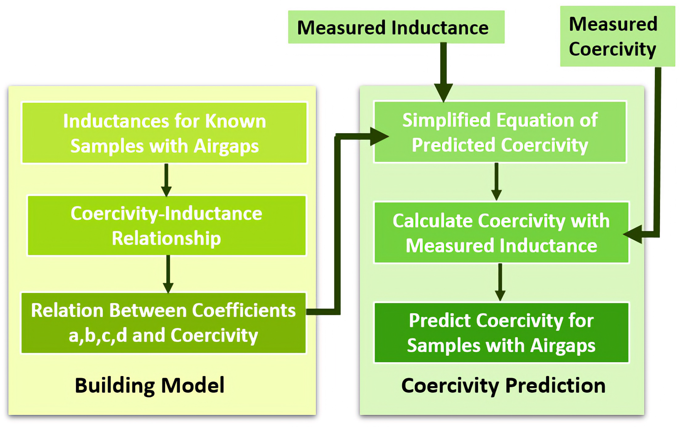
In order to build a coercivity prediction model for different carbon steels, the three-order polynomial relationship between coercivity and the inductances was assumed to be applicable to all materials. Since the coefficients of the polynomial were found to be related to the coercivity of the material, it was possible to calculate the coefficients in terms of coercivity and extrapolate the coercivity–inductance relationship to other samples. The steps of the modeling are shown in Figure 8.

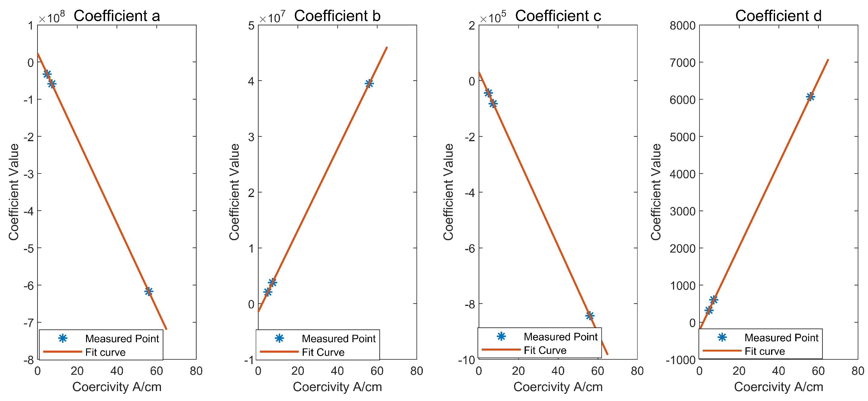
To simplify the model, we assumed that coefficients a, b, c, and d were independent and closely associated with the coercivity of materials. After evaluating various fitting relationships, the coefficients were found to be proportional to coercivity, as shown in Figure 9. The plot displays the coefficients a, b, c, and d for samples A, B, and C. The coefficients have a clear linear relationship with coercivity, as indicated by the fitted curves.

This finding enabled the computation of the coefficients for the predicted coercivity. The linear equations for coefficients a, b, c, and d are:

$$a=K_a{H}_C+R_a$$

(2)

$$b=K_b{H}_C+R_b$$

(3)

$$c=K_c{H}_C+R_c$$

(4)

$$d=K_d{H}_C+R_d$$

(5)

where $K_a$, $K_b$, $K_c$, and $K_d$ are the coefficients for the primary term; $H_c$ represents the base coercivity of the sample; and $R_a$, $R_b$, $R_c$, and $R_d$ are the constant terms of the equation.

By combining Equations (2)–(5) with Equation (1), the measured coercivity $H_m$ becomes:

$$H_c^m=a\left(H_c\right)L_m^3+b\left(H_c\right)L_m^2+c\left(H_c\right)L_m+d\left(H_c\right)$$

(6)

$L_m$ denotes the measured inductance of the sample. With the result of a single measurement, the solution for the predicted base coercivity $H_p$ is

$$H_p=\frac{H_c^m-R}{K_a{L}_m^3+K_b{L}_m^2+K_c{L}_m+K_d}$$

(7)

where R denotes the constant terms calculated using the measured inductance, which can be expressed as

$$R=R_a{L}_m^3+R_b{L}_m^2+R_c{L}_m+R_d$$

(8)

4. Coercivity Correction

In this section, the coercivity of an unknown test sample is deduced when there exists an air gap between the probe and the sample surface.

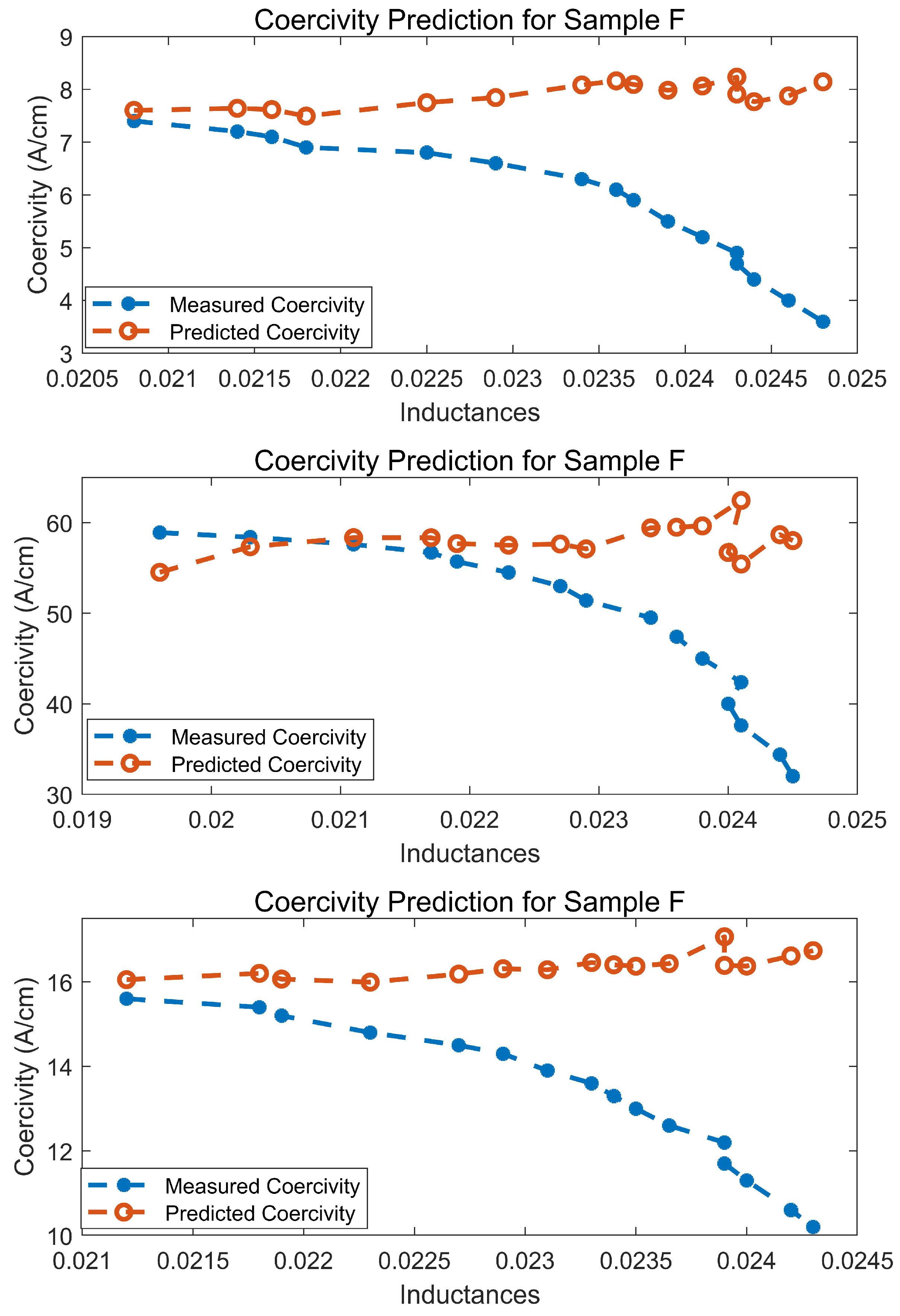
To verify the accuracy of the prediction model, three different new samples (D, E, and F, as shown in

Table 5. Samples and prediction errors.

Test Sample	Sample D	Sample E	Sample F
Coercivity (A/cm)	7.5	58.9	15.6
Mean Predicted Coercivity (A/cm)	7.93	58.01	16.38
Mean Prediction Error	5.17%	2.66%	5.01%
Max Prediction Error	9.33%	7.47%	9.62%

) were employed.

The inductance and coercivity of samples D, E, and F were measured with air gaps ranging from 0 to 15 mm, and the predicted coercivity is shown in Figure 10. As the lift-off increased, the measured coercivity decreased, as expected. The predicted coercivity effectively corrected this deviated coercivity, resulting in successful compensation with a relatively small error (max. prediction error less than 10%).

The small error that persists between the predicted and actual coercivity results may be due to the nature of the non-linear correlation between the inductances and air gaps, particularly for lift-offs exceeding 10 mm, which can lead to prediction errors.

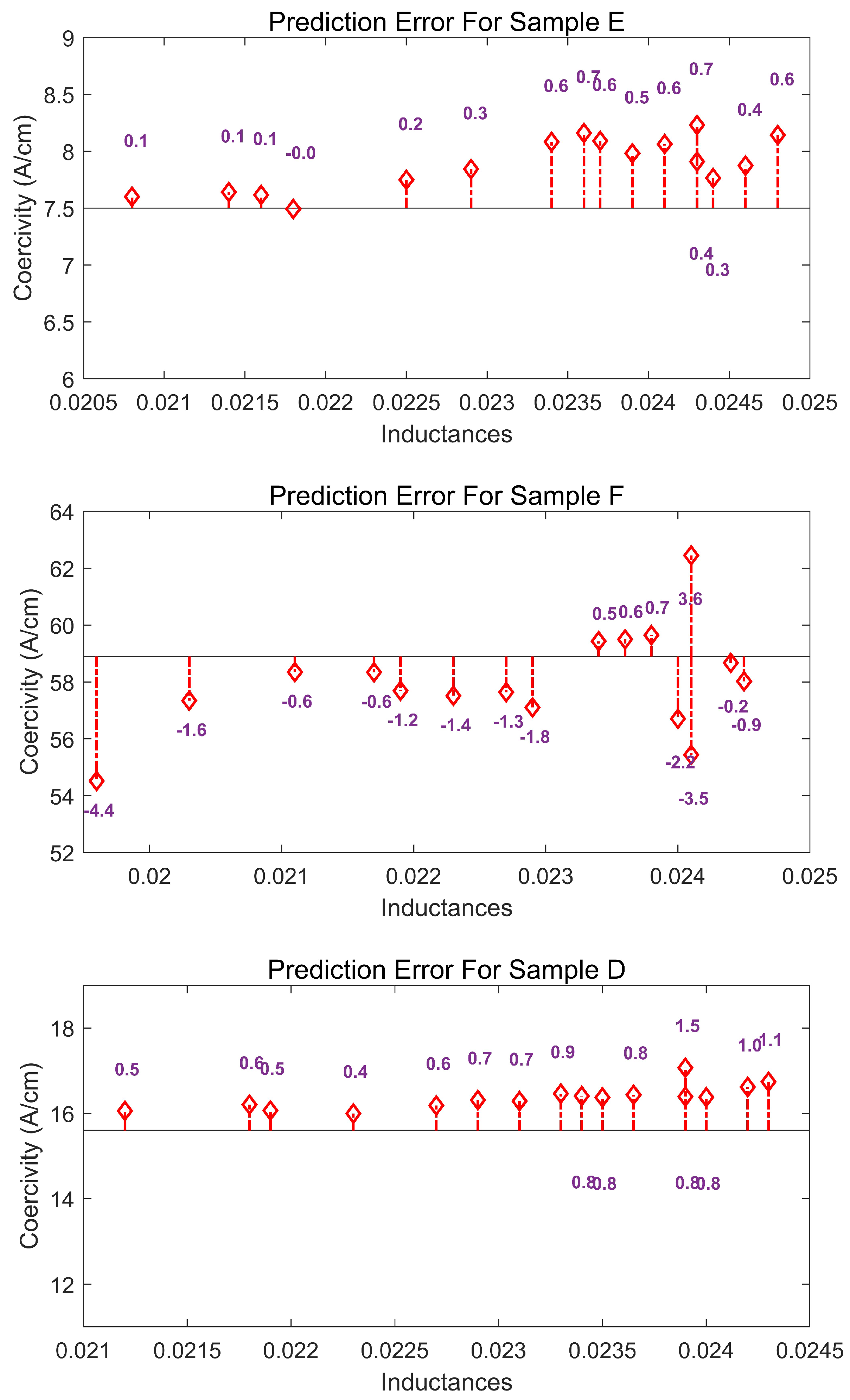
Figure 11 depicts the extent to which the prediction deviated from the actual coercivity. The mean and max. prediction values were calculated, as shown in Table 5. The majority of the predicted values exhibited a small deviation from the base coercivity, with a mean prediction error of less than 6%. Thus, the model can be considered relatively accurate, with a maximum error rate of less than 10%.

5. Conclusions

This paper developed a straightforward model for predicting the coercivities of samples while considering the lift-off effect. The predictions were made using the coercivity measurement results of the samples and the inductances of the excitation coil. The results of this study indicate that the inductance–coercivity relationship curve is a three-order polynomial, and the coefficients are directly proportional to the coercivity of the material, enabling the extrapolation of the coefficients based on the predicted coercivity value. The performance of the model was validated and assessed using three different samples, and the outcomes clearly show that the model succeeded in predicting the coercivity of samples, with an error rate of less than 10%. However, this research was based on a limited number of samples, and the samples were mainly high-carbon steels with different coercivities, which limited the prediction accuracy of the model. Additionally, the performance of the prediction model still needs to be evaluated using other magnetic materials. More samples of different materials will be used to further improve the performance of the model.

References

- Kikuchi, H.; Ara, K.; Kamada, Y.; Kobayashi, S. Effect of Microstructure Changes on Barkhausen Noise Properties and Hysteresis Loop in Cold Rolled Low Carbon Steel. IEEE Trans. Magn. 2009, 45, 2744–2747. [Google Scholar] [CrossRef]
- Liu, J. Magnetic characterisation of microstructural feature distribution in P9 and T22 steels by major and minor BH loop measurements. J. Magn. Magn. Mater. 2016, 401, 579–592. [Google Scholar] [CrossRef]
- Rumiche, F.; Indacochea, J.; Wang, M. Assessment of the Effect of Microstructure on the Magnetic Behavior of Structural Carbon Steels Using an Electromagnetic Sensor. J. Mater. Eng. Perform. 2008, 17, 586–593. [Google Scholar] [CrossRef]
- Kikuchi, H.; Sugai, K.; Murakami, T.; Matsumura, K. Dependence of Coercivity and Barkhausen Noise Signal on Martensitic Stainless Steel with and without Quench. In Studies in Applied Electromagnetics and Mechanics; Tian, G., Gao, B., Eds.; IOS Press: Amsterdam, The Netherlands, 2020; Available online: http://ebooks.iospress.nl/doi/10.3233/SAEM200027 (accessed on 20 July 2023).
- Mitra, A.; Mohapatra, J.; Swaminathan, J.; Ghosh, M.; Panda, A.; Ghosh, R. Magnetic evaluation of creep in modified 9Cr–1Mo steel. Scr. Mater. 2007, 57, 813–816. [Google Scholar]
- Wang, Q.; Cong, G.; Lyu, Y.; Yu, W. A new Cr25Ni35Nb alloy critical failure time prediction method based on coercive force magnetic signature. J. Magn. Magn. Mater. 2022, 549, 168809. [Google Scholar] [CrossRef]
- Stupakov, O. Local Non-contact Evaluation of the ac Magnetic Hysteresis Parameters of Electrical Steels by the Barkhausen Noise Technique. J. Nondestruct. Eval. 2013, 32, 405–412. [Google Scholar]
- Tomas, I.; Kadlecova, J.; Vertesy, G. Measurement of Flat Samples With Rough Surfaces by Magnetic Adaptive Testing. IEEE Trans. Magn. 2012, 48, 1441–1444. [Google Scholar] [CrossRef]
- Matyuk, V.F.; Goncharenko, S.A.; Hartmann, H.; Reichelt, H. Modern State of Nondestructive Testing of Mechanical Properties and Stamping Ability of Steel Sheets in a Manufacturing Technological Flow. Russ. J. Nondestruct. Test. 2003, 39, 347–380. [Google Scholar] [CrossRef]
- Mazaheri-Tehrani, E.; Faiz, J. Airgap and stray magnetic flux monitoring techniques for fault diagnosis of electrical machines: An overview. IET Electr. Power Appl. 2022, 16, 277–299. [Google Scholar] [CrossRef]
- Bida, G.V. The effect of a gap between the poles of an attachable electromagnet and a tested component on coercimeter readings and methods for decreasing it (Review). Russ. J. Nondestruct. Test. 2010, 46, 836–853. [Google Scholar]
- Balakrishnan, A.; Joines, W.T. Air-Gap Reluctance and Inductance Calculations for Magnetic Circuits Using a Schwarz–Christoffel Transformation. IEEE Trans. Power Electron. 1997, 12, 654–663. [Google Scholar] [CrossRef]
- Stupakov, O.; Perevertov, O.; Stoyka, V.; Wood, R. Correlation Between Hysteresis and Barkhausen Noise Parameters of Electrical Steels. IEEE Trans. Magn. 2010, 46, 517–520. [Google Scholar] [CrossRef]
- Lenz, J.; Edelstein, S. Magnetic sensors and their applications. IEEE Sens. J. 2006, 6, 631–649. [Google Scholar] [CrossRef]
- Lenz, J. A review of magnetic sensors. Proc. IEEE 1990, 78, 973–989. [Google Scholar] [CrossRef]
- Ramsden, E. Integrated Sensors: Linear and Digital Devices. In HallEffect Sensors: Theory and Applications; Elsevier: Oxford, UK, 2006. [Google Scholar]
- Zhu, W.; Yin, W.; Peyton, A.; Ploegaert, H. Modelling and experimental study of an electromagnetic sensor with an Hshaped ferrite core used for monitoring the hot transformation of steel in an industrial environment. NDT E Int. 2011, 44, 547–552. [Google Scholar] [CrossRef]