
Review of Fluorescence Lifetime Imaging Microscopy (FLIM) Data Analysis Using Machine Learning


Abstract
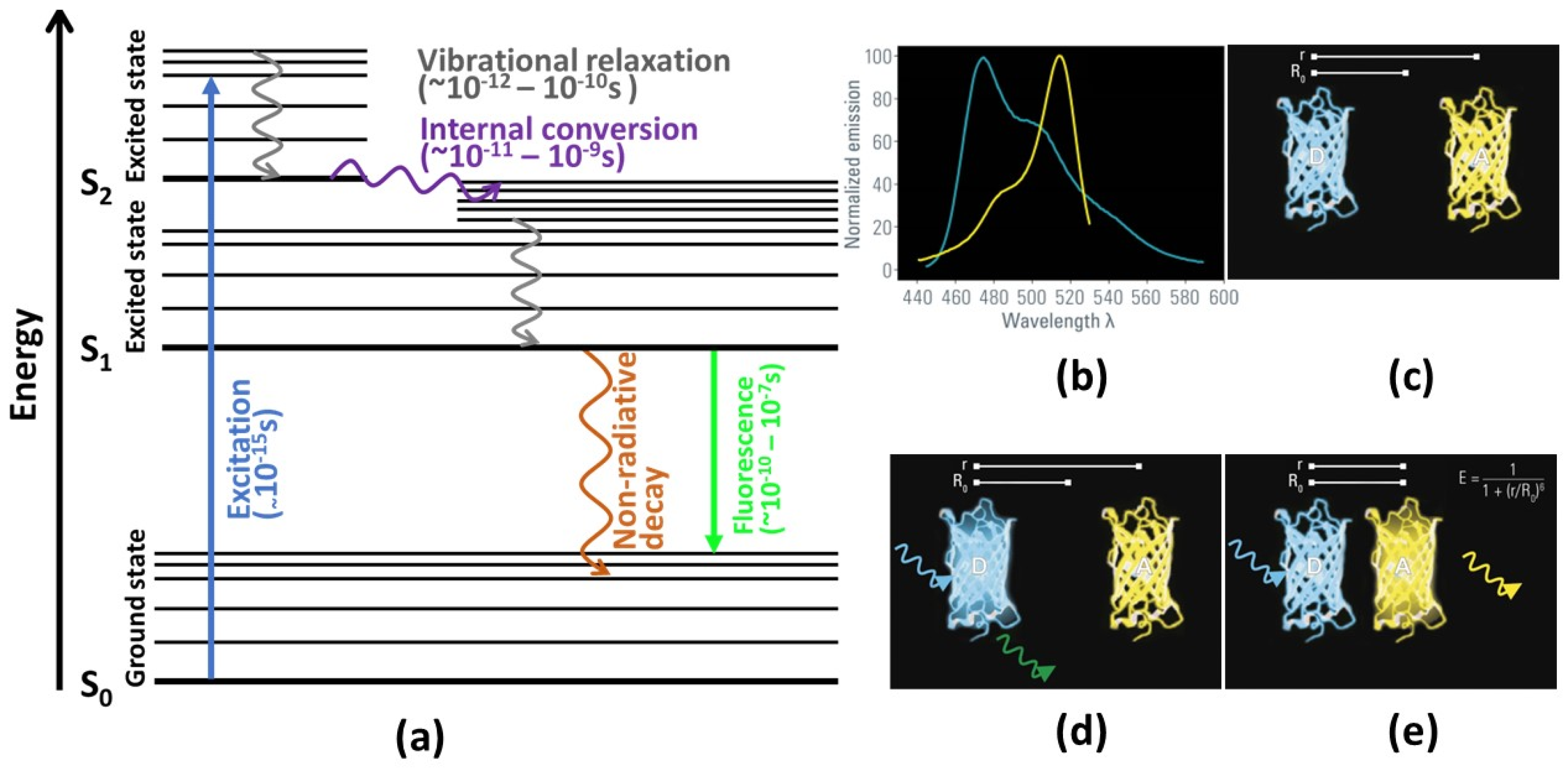
:1. Introduction

2. Preprocessing
3. Data Modeling
3.1. Segmentation
3.2. Classification
3.2.1. Lung Cancer Classification
3.2.2. Skin Cancer Classification
3.2.3. Cervical Cancer Classification
3.2.4. Microglia Classification
3.2.5. Other Classification
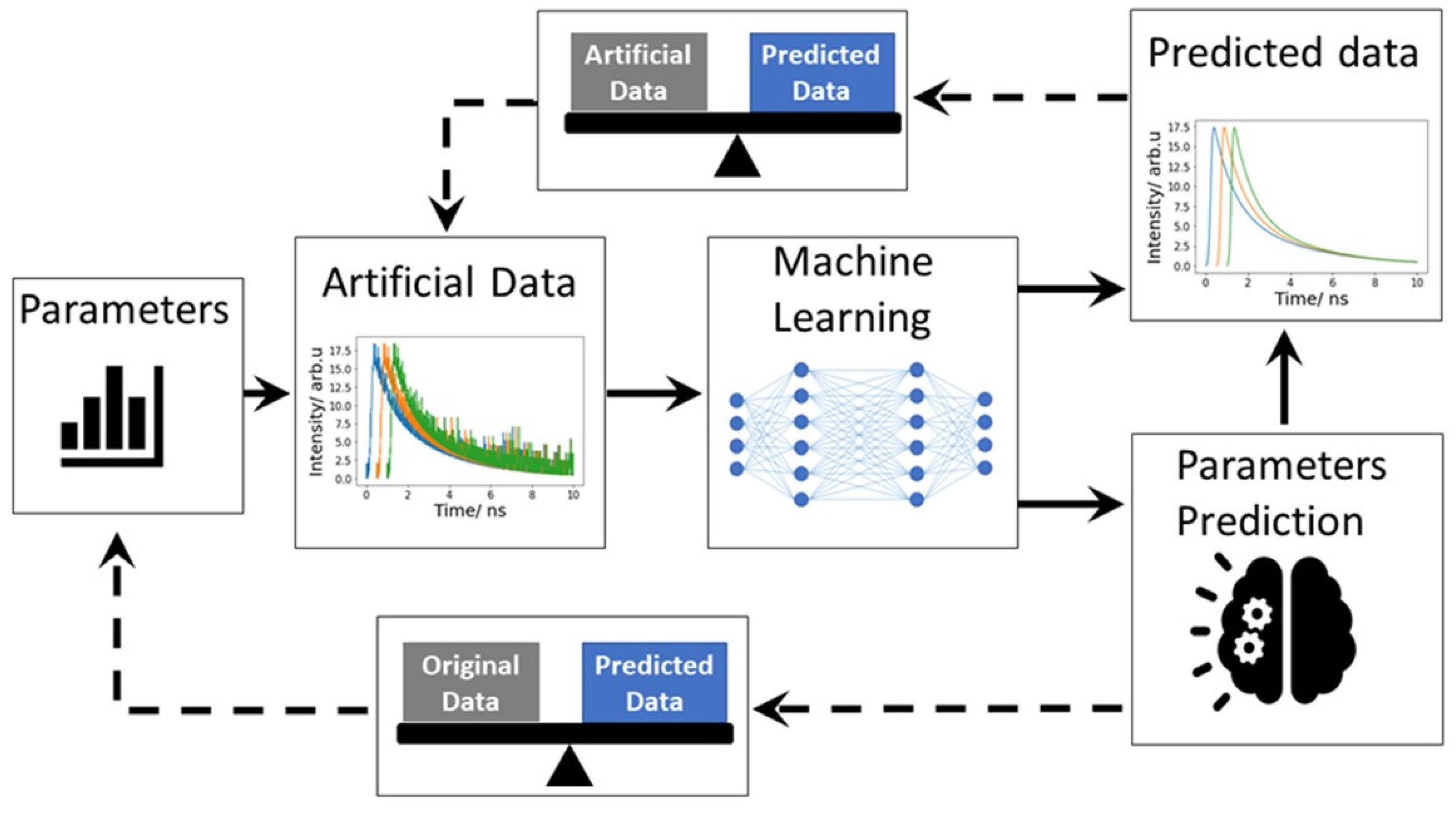
4. Inverse Modeling

| Network Used | Dataset Used | |
|---|---|---|
| Guo et al. [20] | Random forest | Cell sample |
| Wu et al. [59] | ANN with 4 layers. 1—input 1—output 2—hidden | Daisy pollens |
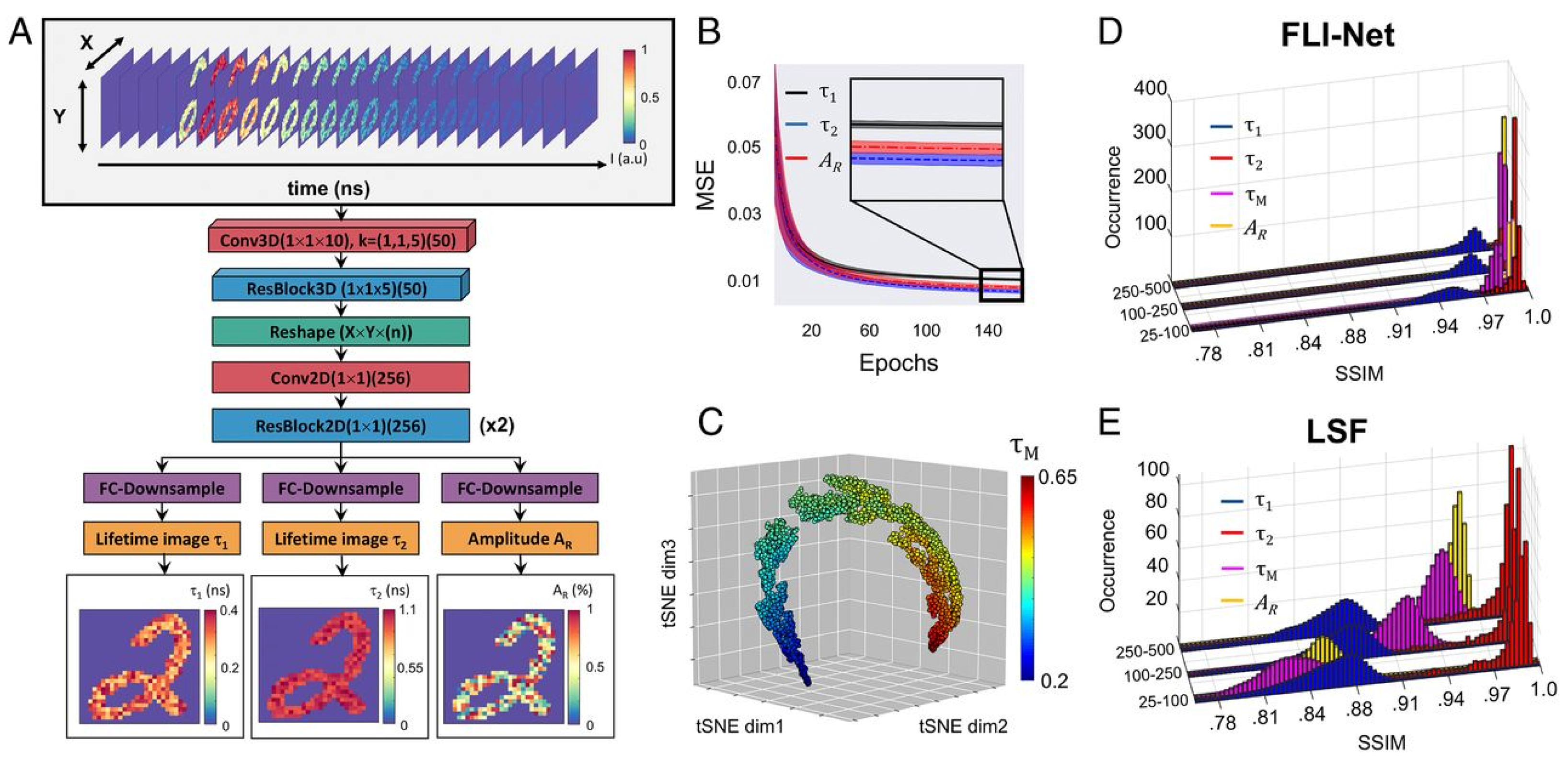
| FLI-Net [60] | 10 layers (combination with convolution and ResNet block) | Mice liver and bladder sample |
| NetFLICS [61] | ResNet | Mice liver and bladder |
| Xiao et al. [63] | Mainly 4 layers. In combination with CNN and ResNetBlock | Human prostate cancer tissue |
5. Discussion and Conclusions
Author Contributions
Funding
Conflicts of Interest
References
- Renz, M. Fluorescence Microscopy—A Historical and Technical Perspective. Cytom. Part A 2013, 83, 767–779. [Google Scholar] [CrossRef] [PubMed]
- Ellinger, P.; Hirt, A. Mikroskopische Untersuchungen an lebenden Organen. Z. Anat. Entwickl. Gesch. 1929, 90, 791–802. [Google Scholar] [CrossRef]
- König, K. 1 Brief History of Fluorescence Lifetime Imaging. In 1 Brief History of Fluorescence Lifetime Imaging; De Gruyter: Berlin, Germany, 2018; pp. 3–16. ISBN 978-3-11-042998-5. [Google Scholar]
- Datta, R.; Heaster, T.M.; Sharick, J.T.; Gillette, A.A.; Skala, M.C. Fluorescence Lifetime Imaging Microscopy: Fundamentals and Advances in Instrumentation, Analysis, and Applications. J. Biomed. Opt. 2020, 25, 071203. [Google Scholar] [CrossRef] [PubMed]
- Lichtman, J.W.; Conchello, J.-A. Fluorescence Microscopy. Nat. Methods 2005, 2, 910–919. [Google Scholar] [CrossRef]
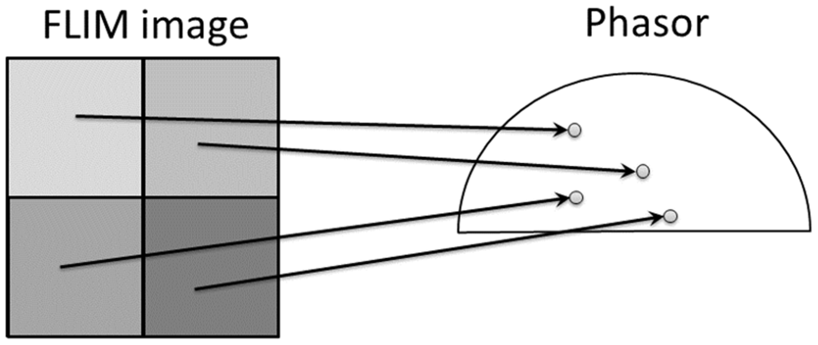
- Ossato, G. Phasor Analysis for FLIM (Fluorescence Lifetime Imaging Microscopy). Available online: https://www.leica-microsystems.com/science-lab/phasor-analysis-for-flim-fluorescence-lifetime-imaging-microscopy/ (accessed on 26 May 2023).
- Bixon, M.; Jortner, J. Intramolecular Radiationless Transitions. J. Chem. Phys. 2003, 48, 715–726. [Google Scholar] [CrossRef]
- Kasha, M. Characterization of Electronic Transitions in Complex Molecules. Discuss. Faraday Soc. 1950, 9, 14–19. [Google Scholar] [CrossRef]
- Bhattacharjee, A.; Datta, R.; Gratton, E.; Hochbaum, A.I. Metabolic Fingerprinting of Bacteria by Fluorescence Lifetime Imaging Microscopy. Sci. Rep. 2017, 7, 3743. [Google Scholar] [CrossRef]
- Kappel, C.; Kuschel, L.; DeRose, J. Was ist FRET mit FLIM (FLIM-FRET)? Available online: https://www.leica-microsystems.com/de/science-lab/life-science/was-ist-fret-mit-flim-flim-fret/ (accessed on 28 August 2023).
- Verveer, P.J.; Gemkow, M.J.; Jovin, T.M. A Comparison of Image Restoration Approaches Applied to Three-Dimensional Confocal and Wide-Field Fluorescence Microscopy. J. Microsc. 1999, 193, 50–61. [Google Scholar] [CrossRef]
- Becker, W. Fluorescence Lifetime Imaging–Techniques and Applications: Fluorescence Lifetime Imaging. J. Microsc. 2012, 247, 119–136. [Google Scholar] [CrossRef]
- Datta, R.; Gillette, A.; Stefely, M.; Skala, M.C. Recent Innovations in Fluorescence Lifetime Imaging Microscopy for Biology and Medicine. J. Biomed. Opt. 2021, 26, 070603. [Google Scholar] [CrossRef]
- Gavin, H.P. The Levenberg-Marquardt Algorithm for Nonlinear Least Squares Curve-Fitting Problems. 2022. Available online: https://people.duke.edu/~hpgavin/ExperimentalSystems/lm.pdf (accessed on 26 May 2023).
- Chessel, A.; Waharte, F.; Salamero, J.; Kervrann, C. A Maximum Likelihood Method for Lifetime Estimation in Photon Counting-Based Fluorescence Lifetime Imaging Microscopy. In Proceedings of the 21st European Signal Processing Conference (EUSIPCO 2013), Marrakech, Morocco, 9–13 September 2013; pp. 1–5. [Google Scholar]
- Maximum Likelihood Estimation|Theory, Assumptions, Properties. Available online: https://www.statlect.com/fundamentals-of-statistics/maximum-likelihood (accessed on 26 May 2023).
- Maus, M.; Cotlet, M.; Hofkens, J.; Gensch, T.; De Schryver, F.C.; Schaffer, J.; Seidel, C.A.M. An Experimental Comparison of the Maximum Likelihood Estimation and Nonlinear Least-Squares Fluorescence Lifetime Analysis of Single Molecules. Anal. Chem. 2001, 73, 2078–2086. [Google Scholar] [CrossRef] [PubMed]
- Pelet, S.; Previte, M.J.R.; Laiho, L.H.; So, P.T.C. A Fast Global Fitting Algorithm for Fluorescence Lifetime Imaging Microscopy Based on Image Segmentation. Biophys. J. 2004, 87, 2807–2817. [Google Scholar] [CrossRef] [PubMed]
- Digman, M.A.; Caiolfa, V.R.; Zamai, M.; Gratton, E. The Phasor Approach to Fluorescence Lifetime Imaging Analysis. Biophys. J. 2008, 94, L14–L16. [Google Scholar] [CrossRef]
- Guo, S.; Silge, A.; Bae, H.; Tolstik, T.; Meyer, T.; Matziolis, G.; Schmitt, M.; Popp, J.; Bocklitz, T. FLIM Data Analysis Based on Laguerre Polynomial Decomposition and Machine-Learning. J. Biomed. Opt. 2021, 26, 022909. [Google Scholar] [CrossRef] [PubMed]
- Tcspc Hand Book, 9th ed.; Becker & Hickl GmbH:: Berlin, Germany, 2021; Available online: https://www.becker-hickl.com/literature/documents/flim/the-bh-tcspc-handbook/ (accessed on 14 September 2023).
- Carrasco Kind, M.; Zurauskas, M.; Alex, A.; Marjanovic, M.; Mukherjee, P.; Doan, M.; Spillman, D.R., Jr.; Hood, S.; Boppart, S.A. Flimview: A Software Framework to Handle, Visualize and Analyze FLIM Data. F1000Research 2020, 9, 574. [Google Scholar] [CrossRef]
- Gao, D.; Barber, P.R.; Chacko, J.V.; Kader Sagar, M.A.; Rueden, C.T.; Grislis, A.R.; Hiner, M.C.; Eliceiri, K.W. FLIMJ: An Open-Source ImageJ Toolkit for Fluorescence Lifetime Image Data Analysis. PLoS ONE 2020, 15, e0238327. [Google Scholar] [CrossRef]
- FLIMfit. Available online: https://flimfit.org/ (accessed on 26 May 2023).
- Zhang, Y.; Zhu, Y.; Nichols, E.; Wang, Q.; Zhang, S.; Smith, C.; Howard, S. A Poisson-Gaussian Denoising Dataset with Real Fluorescence Microscopy Images. In Proceedings of the 2019 IEEE/CVF Conference on Computer Vision and Pattern Recognition (CVPR), Long Beach, CA, USA, 15–20 June 2019; pp. 11702–11710. [Google Scholar]
- Zhong, L.; Liu, G.; Yang, G. Blind Denoising of Fluorescence Microscopy Images Using GAN-Based Global Noise Modeling. In Proceedings of the 2021 IEEE 18th International Symposium on Biomedical Imaging (ISBI), Nice, France, 13–16 April 2021; IEEE: Piscataway, NJ, USA, 2021; pp. 863–867. [Google Scholar]
- Lebrun, M. An Analysis and Implementation of the BM3D Image Denoising Method. Image Process. Line 2012, 2, 175–213. [Google Scholar] [CrossRef]
- Zhang, K.; Zuo, W.; Chen, Y.; Meng, D.; Zhang, L. Beyond a Gaussian Denoiser: Residual Learning of Deep CNN for Image Denoising. IEEE Trans. Image Process. 2017, 26, 3142–3155. [Google Scholar] [CrossRef]
- Aharon, M.; Elad, M.; Bruckstein, A. K-SVD: An Algorithm for Designing Overcomplete Dictionaries for Sparse Representation. IEEE Trans. Signal Process. 2006, 54, 4311–4322. [Google Scholar] [CrossRef]
- Li, J.; Luisier, F.; Blu, T. PURE-LET Image Deconvolution. IEEE Trans. Image Process. 2018, 27, 92–105. [Google Scholar] [CrossRef] [PubMed]
- Belthangady, C.; Royer, L.A. Applications, Promises, and Pitfalls of Deep Learning for Fluorescence Image Reconstruction. Nat. Methods 2019, 16, 1215–1225. [Google Scholar] [CrossRef] [PubMed]
- Weigert, M.; Schmidt, U.; Boothe, T.; Müller, A.; Dibrov, A.; Jain, A.; Wilhelm, B.; Schmidt, D.; Broaddus, C.; Culley, S.; et al. Content-Aware Image Restoration: Pushing the Limits of Fluorescence Microscopy. Nat. Methods 2018, 15, 1090–1097. [Google Scholar] [CrossRef] [PubMed]
- Batson, J.; Royer, L. Noise2Self: Blind Denoising by Self-Supervision. In Proceedings of the 36th International Conference on Machine Learning, Long Beach, CA, USA, 9–15 June 2019; pp. 524–533. [Google Scholar]
- Mannam, V.; Zhang, Y.; Yuan, X.; Hato, T.; Dagher, P.C.; Nichols, E.L.; Smith, C.J.; Dunn, K.W.; Howard, S. Convolutional Neural Network Denoising in Fluorescence Lifetime Imaging Microscopy (FLIM). In Proceedings of the Multiphoton Microscopy in the Biomedical Sciences XXI, Online. 5–12 March 2021; p. 43. [Google Scholar]
- Suykens, J.A.K.; Vandewalle, J.P.L.; De Moor, B.L.R. Artificial Neural Networks: Architectures and Learning Rules. In Artificial Neural Networks for Modelling and Control of Non-Linear Systems; Suykens, J.A.K., Vandewalle, J.P.L., De Moor, B.L.R., Eds.; Springer: Boston, MA, USA, 1996; pp. 19–35. ISBN 978-1-4757-2493-6. [Google Scholar]
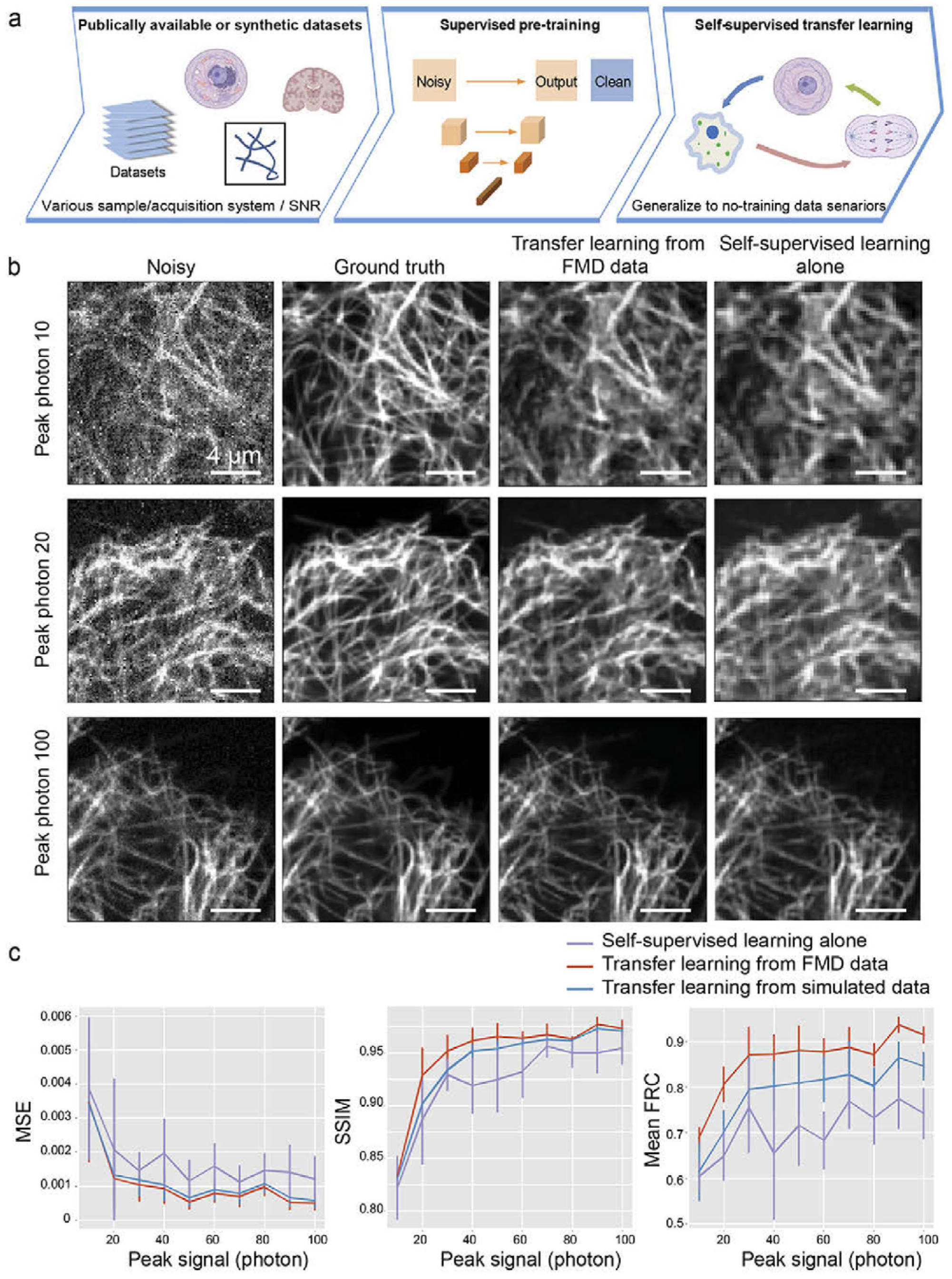
- Wang, Y.; Pinkard, H.; Khwaja, E.; Zhou, S.; Waller, L.; Huang, B. Image Denoising for Fluorescence Microscopy by Supervised to Self-Supervised Transfer Learning. Opt. Express 2021, 29, 41303–41312. [Google Scholar] [CrossRef]
- Zhang, Y.; Hato, T.; Dagher, P.C.; Nichols, E.L.; Smith, C.J.; Dunn, K.W.; Howard, S.S. Automatic Segmentation of Intravital Fluorescence Microscopy Images by K-Means Clustering of FLIM Phasors. Opt. Lett. 2019, 44, 3928. [Google Scholar] [CrossRef]
- Ji, M.; Zhong, J.; Xue, R.; Su, W.; Kong, Y.; Fei, Y.; Ma, J.; Wang, Y.; Mi, L. Early Detection of Cervical Cancer by Fluorescence Lifetime Imaging Microscopy Combined with Unsupervised Machine Learning. Int. J. Mol. Sci. 2022, 23, 11476. [Google Scholar] [CrossRef]
- Otsu, N. A Threshold Selection Method from Gray-Level Histograms. IEEE Trans. Syst. Man Cybern. 1979, 9, 62–66. [Google Scholar] [CrossRef]
- Wang, Q.; Vallejo, M.; Hopgood, J. Fluorescence Lifetime Endomicroscopic Image-Based Ex-Vivo Human Lung Cancer Differentiation Using Machine Learning. TechRxiv Preprint 2020. [Google Scholar] [CrossRef]
- Wang, M.; Tang, F.; Pan, X.; Yao, L.; Wang, X.; Jing, Y.; Ma, J.; Wang, G.; Mi, L. Rapid Diagnosis and Intraoperative Margin Assessment of Human Lung Cancer with Fluorescence Lifetime Imaging Microscopy. BBA Clin. 2017, 8, 7–13. [Google Scholar] [CrossRef]
- Wang, Q.; Hopgood, J.R.; Finlayson, N.; Williams, G.O.S.; Fernandes, S.; Williams, E.; Akram, A.; Dhaliwal, K.; Vallejo, M. Deep Learning in Ex-Vivo Lung Cancer Discrimination Using Fluorescence Lifetime Endomicroscopic Images. In Proceedings of the 2020 42nd Annual International Conference of the IEEE Engineering in Medicine & Biology Society (EMBC), Montreal, QC, Canada, 20–24 July 2020; IEEE: Piscataway, NJ, USA, 2020; pp. 1891–1894. [Google Scholar]
- Wang, Q.; Hopgood, J.R.; Vallejo, M. Fluorescence Lifetime Imaging Endomicroscopy Based Ex-Vivo Lung Cancer Prediction Using Multi-Scale Concatenated-Dilation Convolutional Neural Networks. In Proceedings of the Medical Imaging 2021: Computer-Aided Diagnosis, Online. 15–20 February 2021; Drukker, K., Mazurowski, M.A., Eds.; SPIE: Bellingham, WA, USA, 2021; p. 94. [Google Scholar]
- He, K.; Zhang, X.; Ren, S.; Sun, J. Deep Residual Learning for Image Recognition. arXiv 2015, arXiv:1512.03385. [Google Scholar] [CrossRef]
- Huang, G.; Liu, Z.; van der Maaten, L.; Weinberger, K.Q. Densely Connected Convolutional Networks. arXiv 2018, arXiv:1608.06993. [Google Scholar] [CrossRef]
- Wang, Q.; Hopgood, J.R.; Fernandes, S.; Finlayson, N.; Williams, G.O.S.; Akram, A.R.; Dhaliwal, K.; Vallejo, M. A Layer-Level Multi-Scale Architecture for Lung Cancer Classification with Fluorescence Lifetime Imaging Endomicroscopy. Neural Comput. Appl. 2022, 34, 18881–18894. [Google Scholar] [CrossRef]
- Gao, S.-H.; Cheng, M.-M.; Zhao, K.; Zhang, X.-Y.; Yang, M.-H.; Torr, P. Res2Net: A New Multi-Scale Backbone Architecture. IEEE Trans. Pattern Anal. Mach. Intell. 2021, 43, 652–662. [Google Scholar] [CrossRef] [PubMed]
- Yang, Q.; Qi, M.; Wu, Z.; Liu, L.; Gao, P.; Qu, J. Classification of Skin Cancer Based on Fluorescence Lifetime Imaging and Machine Learning. In Proceedings of the Optics in Health Care and Biomedical Optics X, Online. 11–16 October 2020; Luo, Q., Li, X., Gu, Y., Zhu, D., Eds.; SPIE: Bellingham, WA, USA, 2020; p. 71. [Google Scholar]
- Chen, B.; Lu, Y.; Pan, W.; Xiong, J.; Yang, Z.; Yan, W.; Liu, L.; Qu, J. Support Vector Machine Classification of Nonmelanoma Skin Lesions Based on Fluorescence Lifetime Imaging Microscopy. Anal. Chem. 2019, 91, 10640–10647. [Google Scholar] [CrossRef] [PubMed]
- Sung, H.; Ferlay, J.; Siegel, R.L.; Laversanne, M.; Soerjomataram, I.; Jemal, A.; Bray, F. Global Cancer Statistics 2020: GLOBOCAN Estimates of Incidence and Mortality Worldwide for 36 Cancers in 185 Countries. CA Cancer J. Clin. 2021, 71, 209–249. [Google Scholar] [CrossRef] [PubMed]
- Jun, G.; Koon, N.B.; Yaw, F.C.; s/o Gulam Razul, S.; Kim, L.S. Fluorescence Lifetime Diagnosis of Cervical Cancer Based on Extreme Learning Machine. In Proceedings of the 2010 Photonics Global Conference, Orchard, Singapore, 14–16 December 2010; IEEE: Piscataway, NJ, USA, 2010; pp. 1–3. [Google Scholar]
- Gu, J.; Fu, C.Y.; Ng, B.K.; Liu, L.B.; Lim-Tan, S.K.; Lee, C.G.L. Enhancement of Early Cervical Cancer Diagnosis with Epithelial Layer Analysis of Fluorescence Lifetime Images. PLoS ONE 2015, 10, e0125706. [Google Scholar] [CrossRef]
- Wei, J. AlexNet: The Architecture That Challenged CNNs. Available online: https://towardsdatascience.com/alexnet-the-architecture-that-challenged-cnns-e406d5297951 (accessed on 26 May 2023).
- Sagar, M.A.K.; Cheng, K.P.; Ouellette, J.N.; Williams, J.C.; Watters, J.J.; Eliceiri, K.W. Machine Learning Methods for Fluorescence Lifetime Imaging (FLIM) Based Label-Free Detection of Microglia. Front. Neurosci. 2020, 14, 931. [Google Scholar] [CrossRef]
- Jo, J.A.; Cheng, S.; Cuenca-Martinez, R.; Duran-Sierra, E.; Malik, B.; Ahmed, B.; Maitland, K.; Cheng, Y.-S.L.; Wright, J.; Reese, T. Endogenous Fluorescence Lifetime Imaging (FLIM) Endoscopy for Early Detection of Oral Cancer and Dysplasia. In Proceedings of the 2018 40th Annual International Conference of the IEEE Engineering in Medicine and Biology Society (EMBC), Honolulu, HI, USA, 18–21 July 2018; IEEE: Piscataway, NJ, USA, 2018; pp. 3009–3012. [Google Scholar]
- Walsh, A.J.; Mueller, K.; Jones, I.; Walsh, C.M.; Piscopo, N.; Niemi, N.N.; Pagliarini, D.J.; Saha, K.; Skala, M.C. Label-Free Method for Classification of T Cell Activation. bioRxiv 2019. [Google Scholar] [CrossRef]
- Marsden, M.; Weaver, S.S.; Marcu, L.; Campbell, M.J. Intraoperative Mapping of Parathyroid Glands Using Fluorescence Lifetime Imaging. J. Surg. Res. 2021, 265, 42–48. [Google Scholar] [CrossRef]
- Zang, Z.; Xiao, D.; Wang, Q.; Jiao, Z.; Chen, Y.; Li, D.D.U. Compact and Robust Deep Learning Architecture for Fluorescence Lifetime Imaging and FPGA Implementation. Methods Appl. Fluoresc. 2023, 11, 025002. [Google Scholar] [CrossRef]
- Wu, G.; Nowotny, T.; Zhang, Y.; Yu, H.-Q.; Li, D.D.-U. Artificial Neural Network Approaches for Fluorescence Lifetime Imaging Techniques. Opt. Lett. 2016, 41, 2561. [Google Scholar] [CrossRef]
- Smith, J.T.; Yao, R.; Sinsuebphon, N.; Rudkouskaya, A.; Un, N.; Mazurkiewicz, J.; Barroso, M.; Yan, P.; Intes, X. Fast Fit-Free Analysis of Fluorescence Lifetime Imaging via Deep Learning. Proc. Natl. Acad. Sci. USA 2019, 116, 24019–24030. [Google Scholar] [CrossRef] [PubMed]
- Yao, R.; Ochoa, M.; Yan, P.; Intes, X. Net-FLICS: Fast Quantitative Wide-Field Fluorescence Lifetime Imaging with Compressed Sensing—A Deep Learning Approach. Light Sci. Appl. 2019, 8, 26. [Google Scholar] [CrossRef]
- Zickus, V.; Wu, M.-L.; Morimoto, K.; Kapitany, V.; Fatima, A.; Turpin, A.; Insall, R.; Whitelaw, J.; Machesky, L.; Bruschini, C.; et al. Fluorescence Lifetime Imaging with a Megapixel SPAD Camera and Neural Network Lifetime Estimation. Sci. Rep. 2020, 10, 20986. [Google Scholar] [CrossRef]
- Xiao, D.; Chen, Y.; Li, D.D.-U. One-Dimensional Deep Learning Architecture for Fast Fluorescence Lifetime Imaging. IEEE J. Sel. Top. Quantum Electron. 2021, 27, 1–10. [Google Scholar] [CrossRef]
- Xiao, D.; Sapermsap, N.; Chen, Y.; Li, D.D.U. Deep learning enhanced fast fluorescence lifetime imaging with a few photons. Optica 2023, 10, 944–951. [Google Scholar] [CrossRef]
- Ochoa, M.; Rudkouskaya, A.; Yao, R.; Yan, P.; Barroso, M.; Intes, X. Deep Learning Enhanced Hyperspectral Fluorescence Lifetime Imaging. bioRxiv 2020. [Google Scholar] [CrossRef]


| Protein–protein interaction studies | FLIM can be used to investigate protein–protein interactions based on FRET. |
| This helps in understanding dynamic protein complexes and signaling pathways within living cells. | |
| Cellular metabolism analysis | FLIM can monitor the autofluorescence of cellular metabolites like NAD(P)H and FAD. |
| The changes in these metabolites can indicate an alteration in cellular energy production. | |
| Live-cell imaging and biomedical applications | FLIM can be used as a non-invasive live cell imaging, providing information about cellular analysis and molecular interaction. |
| FLIM can provide useful information in biomedical research. | |
| Super-resolution microscopy | FLIM can be integrated with super-resolution microscopy techniques like STED-FCS to achieve higher-resolution imaging. |
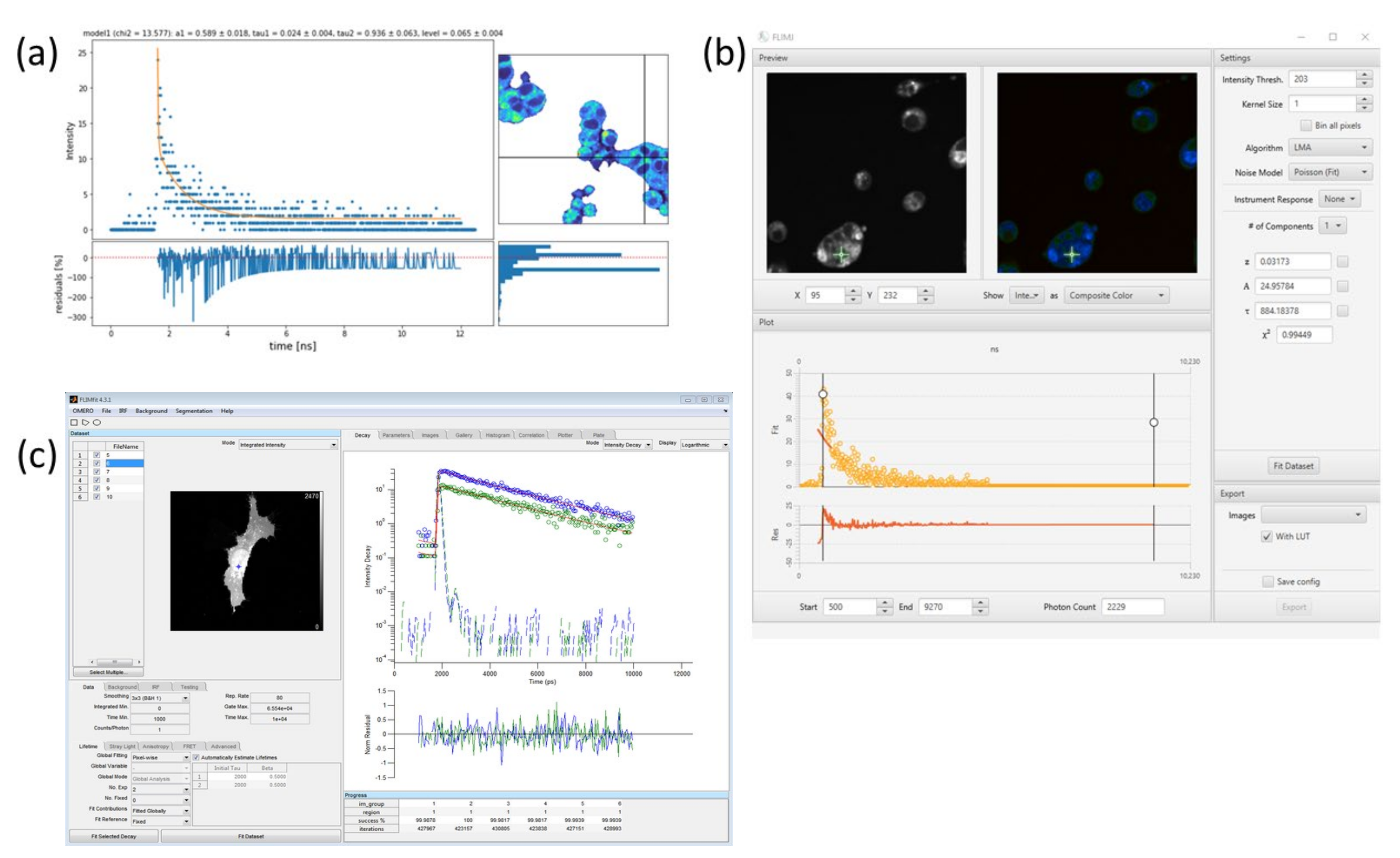
| FLIMview [22] | FLIMJ [23] | FLIMfit [24] |
|---|---|---|
| Based on Python | ImageJ Plugin | Based on MATLAB |
| Support for file formats .std and .ptu. Curve-fitting routines are implemented | Fitting routines for lifetime data based on Levenberg–Marquardt curve fitting, Bayesian and phasor analysis, and rapid lifetime determination methods | Omero client: It can load some specific data formats, like .std, .txt, .tif, .raw. Fitted parameters can be exported as .csv |
Disclaimer/Publisher’s Note: The statements, opinions and data contained in all publications are solely those of the individual author(s) and contributor(s) and not of MDPI and/or the editor(s). MDPI and/or the editor(s) disclaim responsibility for any injury to people or property resulting from any ideas, methods, instructions or products referred to in the content. |
© 2023 by the authors. Licensee MDPI, Basel, Switzerland. This article is an open access article distributed under the terms and conditions of the Creative Commons Attribution (CC BY) license (https://creativecommons.org/licenses/by/4.0/).
Share and Cite
Adhikari, M.; Houhou, R.; Hniopek, J.; Bocklitz, T. Review of Fluorescence Lifetime Imaging Microscopy (FLIM) Data Analysis Using Machine Learning. J. Exp. Theor. Anal. 2023, 1, 44-63. https://doi.org/10.3390/jeta1010004
Adhikari M, Houhou R, Hniopek J, Bocklitz T. Review of Fluorescence Lifetime Imaging Microscopy (FLIM) Data Analysis Using Machine Learning. Journal of Experimental and Theoretical Analyses. 2023; 1(1):44-63. https://doi.org/10.3390/jeta1010004
Chicago/Turabian StyleAdhikari, Mou, Rola Houhou, Julian Hniopek, and Thomas Bocklitz. 2023. "Review of Fluorescence Lifetime Imaging Microscopy (FLIM) Data Analysis Using Machine Learning" Journal of Experimental and Theoretical Analyses 1, no. 1: 44-63. https://doi.org/10.3390/jeta1010004