
Geometrical Analysis of an Oscillating Water Column Converter Device Considering Realistic Irregular Wave Generation with Bathymetry

 ,
,  , , , , ,
  and
and
Abstract
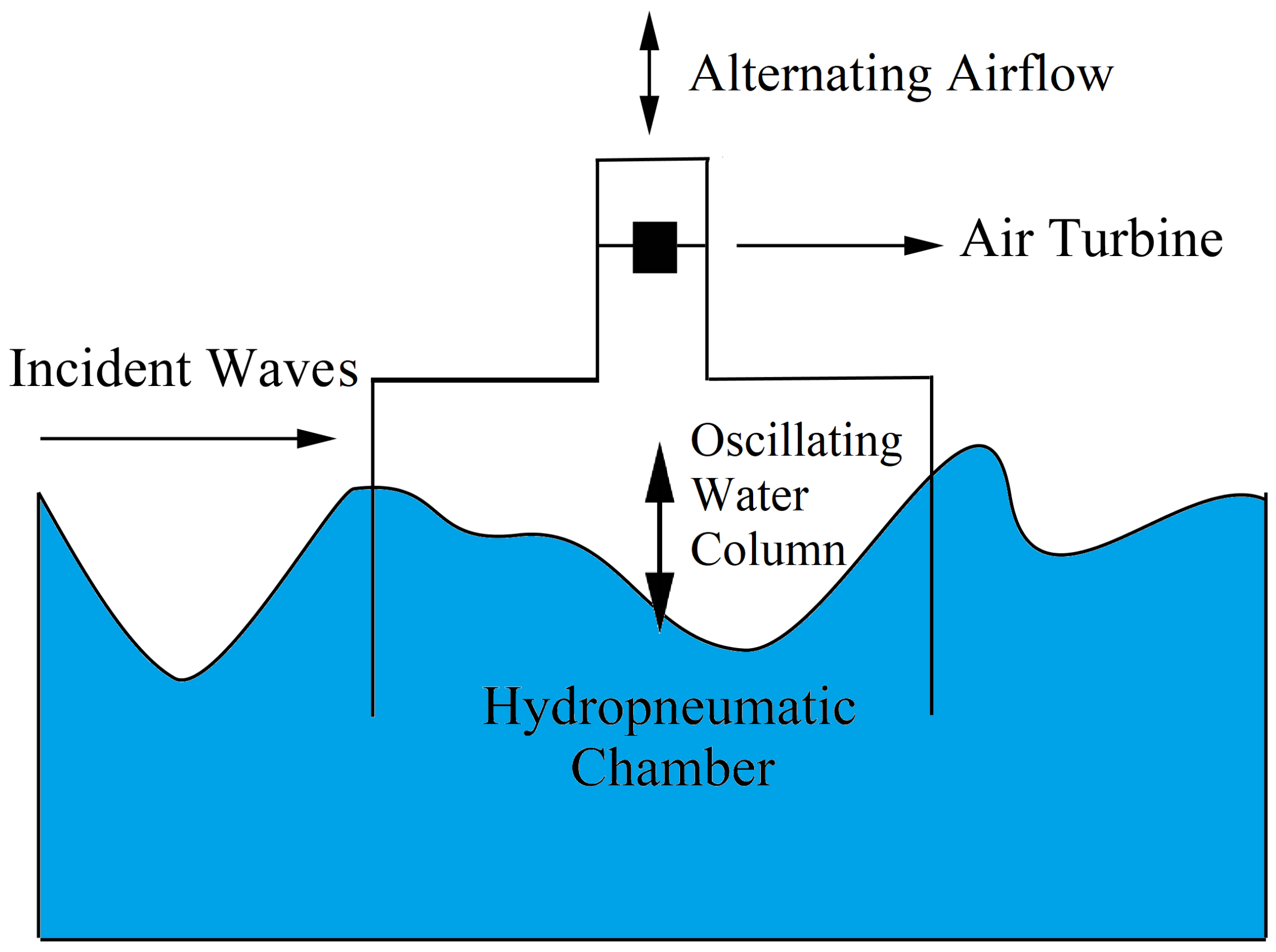
:1. Introduction
2. Materials and Methods
2.1. Mathematical and Numerical Modeling
2.2. WaveMIMO Methodology
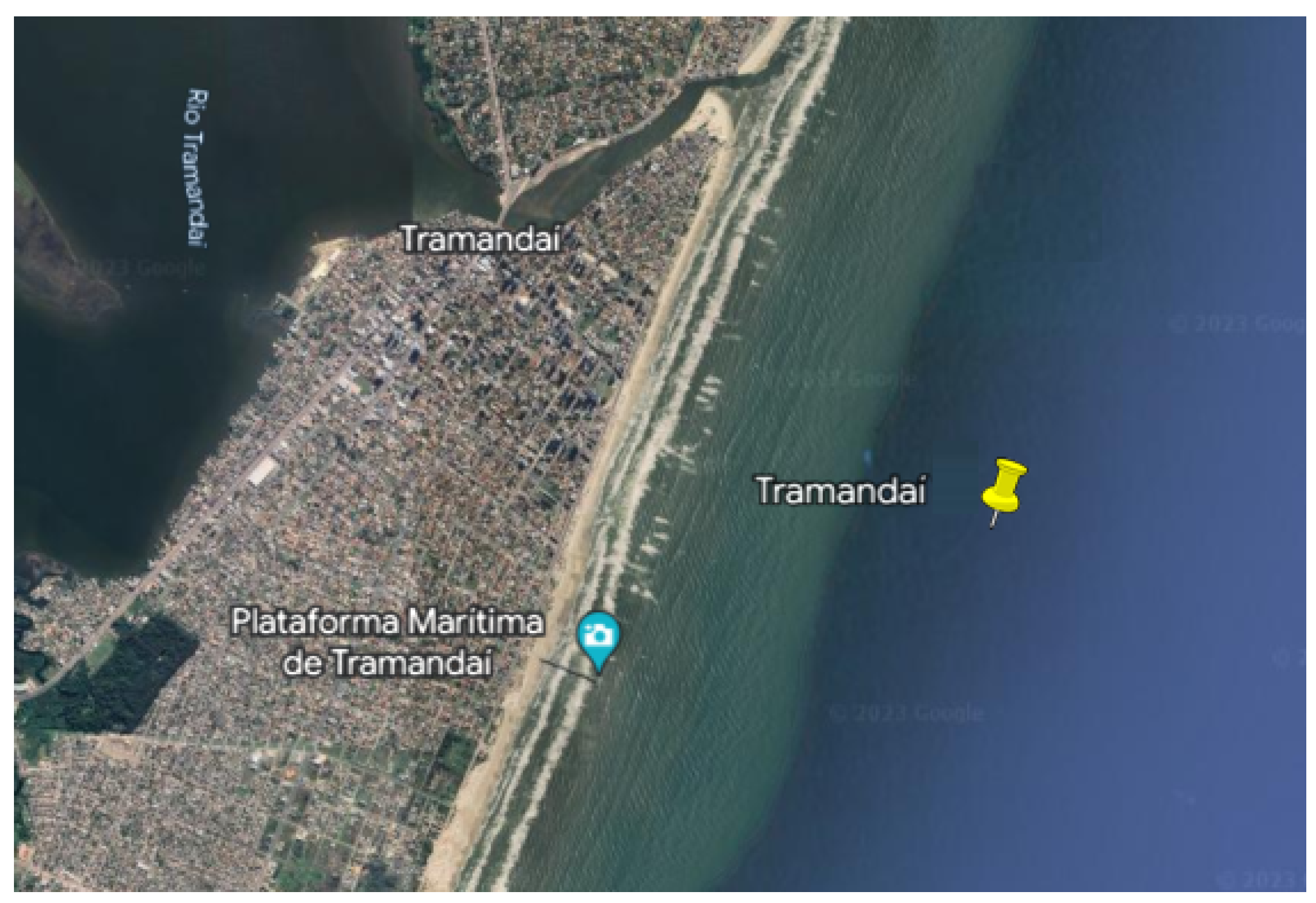
- Location and time of study: a place and a time interval were chosen, and, thus, a simulation of the sea state was performed with these conditions.
- TOMAWAC: the software was used for the numerical simulation of the sea state.
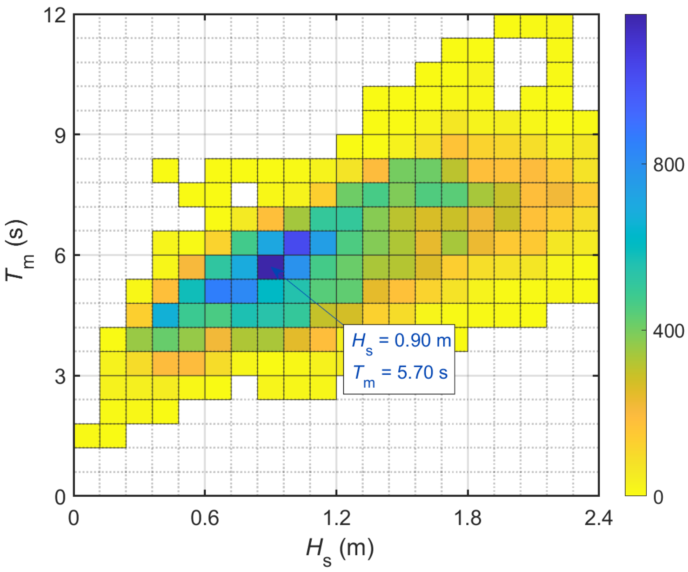
- Wave spectrum simulation: a wave spectrum was extracted from the sea state simulation at the chosen location and time interval.
- Spectral data conversion: the wave spectrum was transformed into a free surface elevation time series statistically identical to the initial wave spectrum, thus representing the sea state [33].
- Orbital velocities u and w: velocity profiles were imposed as boundary conditions in Fluent to generate a realistic sea state.
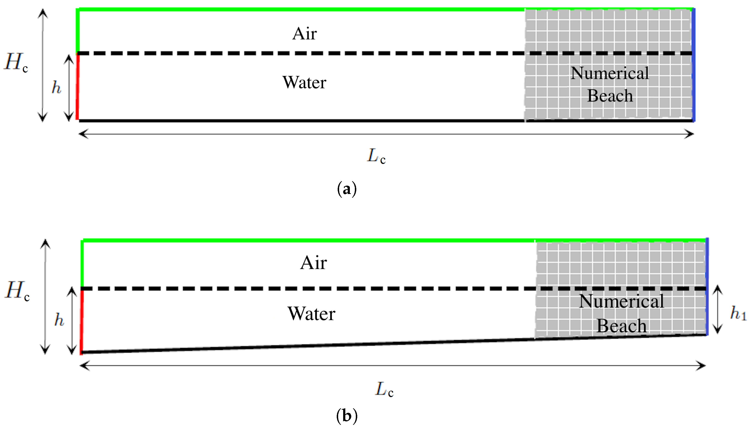
Bathymetry Influence Study and Numerical Model Verification
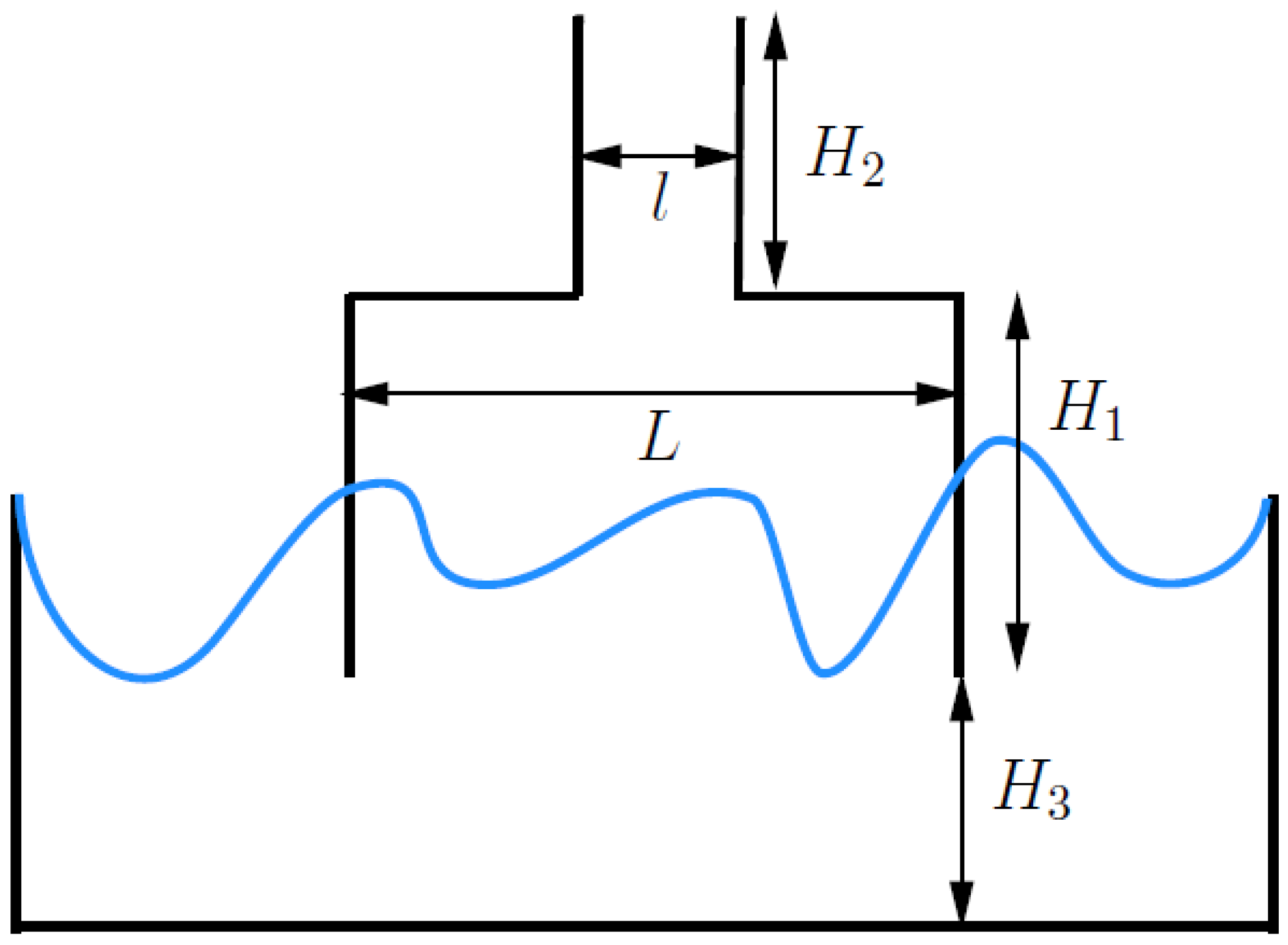
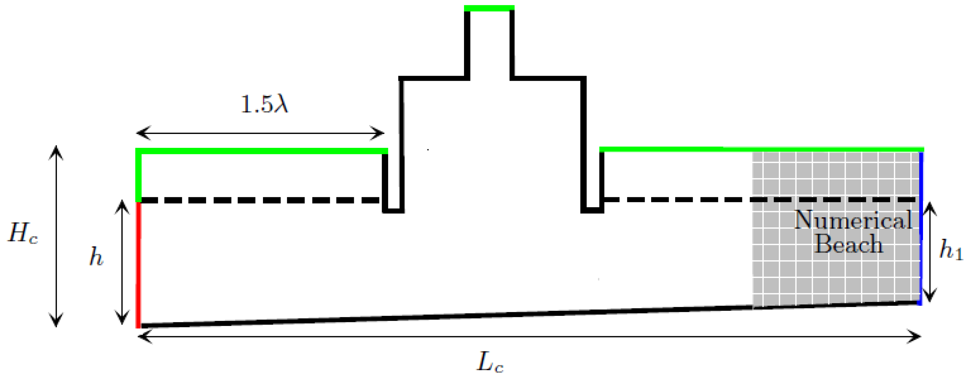
2.3. Geometric Optimization of OWC WEC
2.4. Error Metrics
3. Results and Discussion
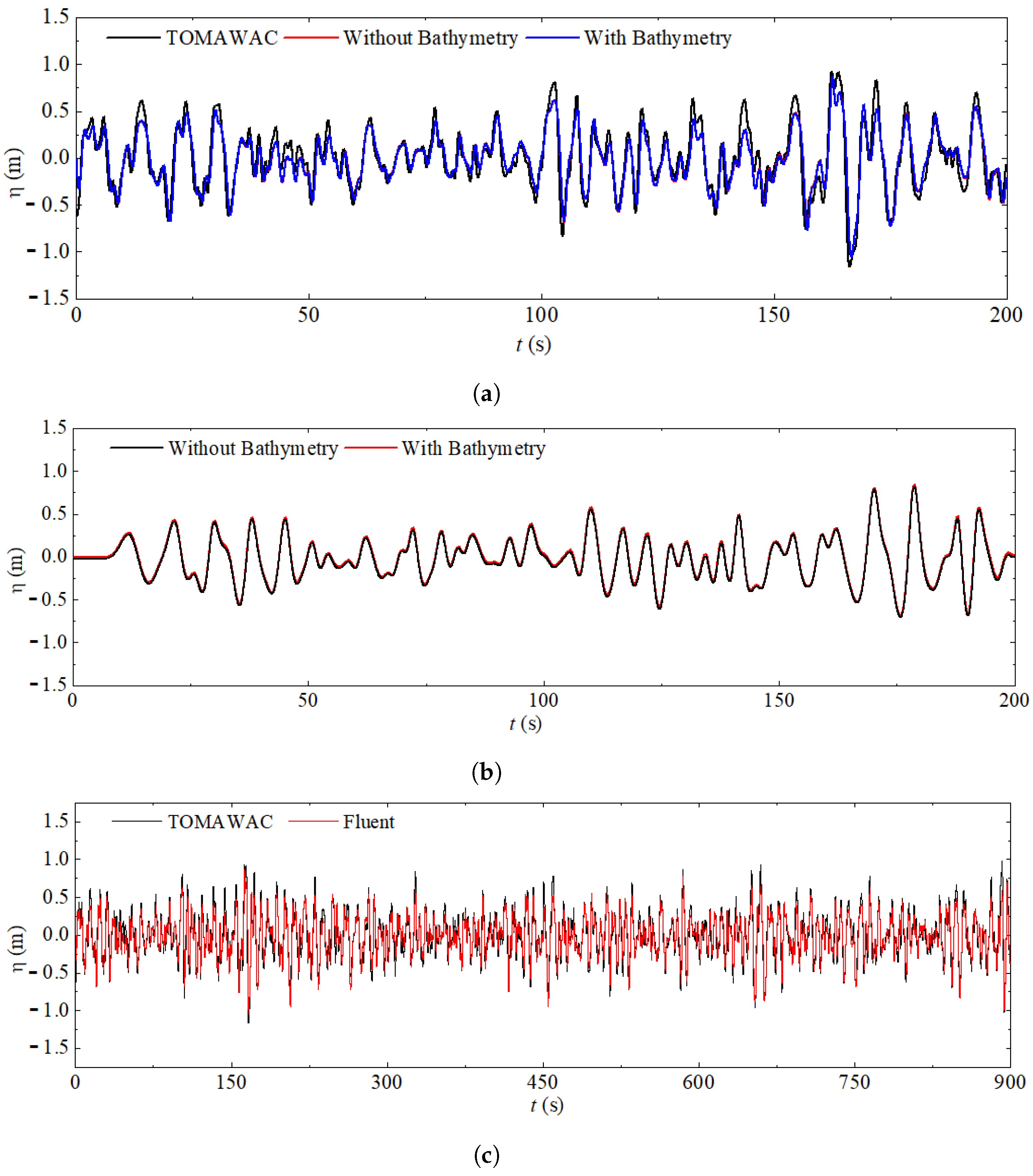
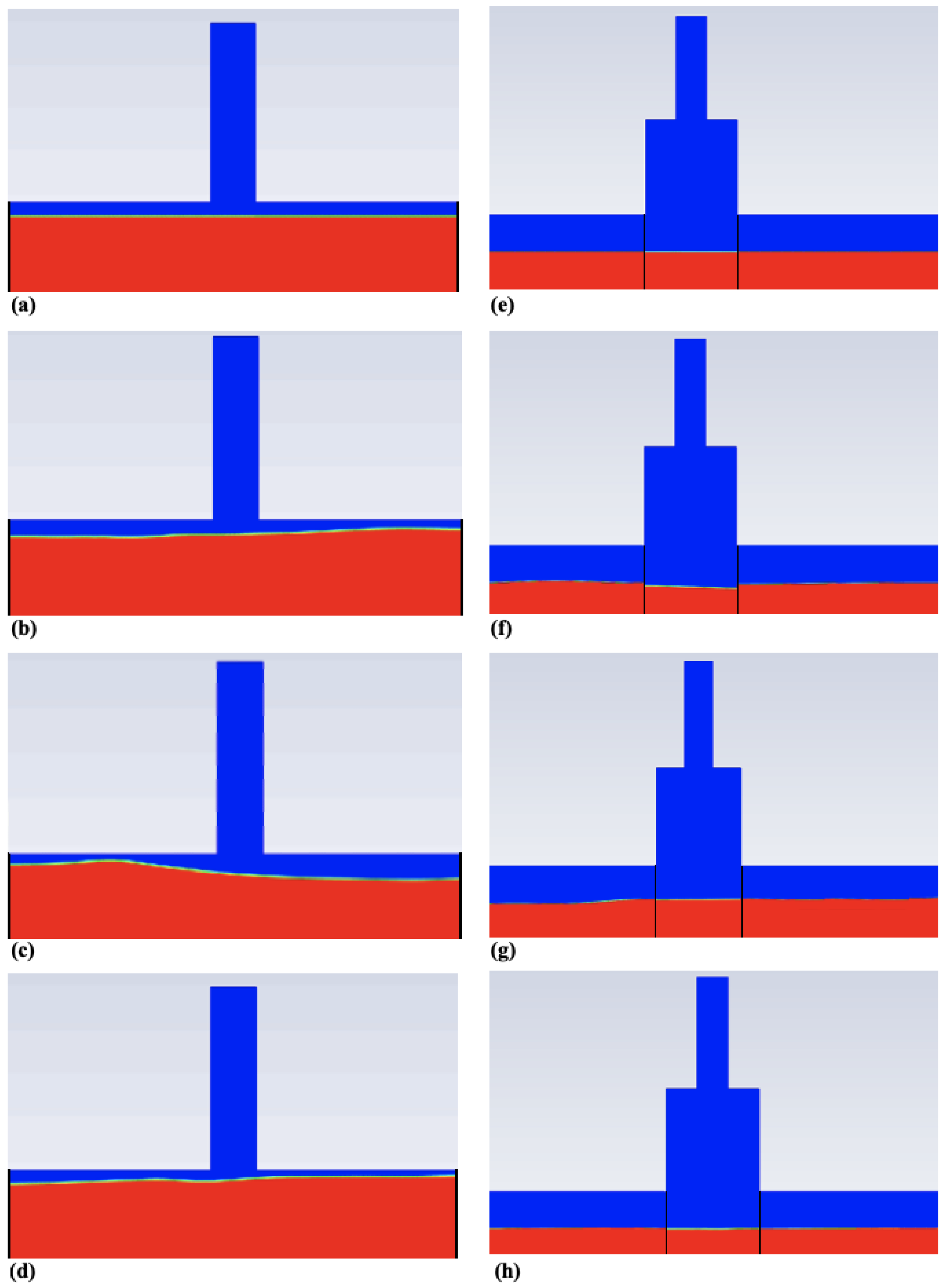
3.1. Study of Bathymetry Influence in the Generation and Propagation of Realistic Irregular Waves and Numerical Model Verification
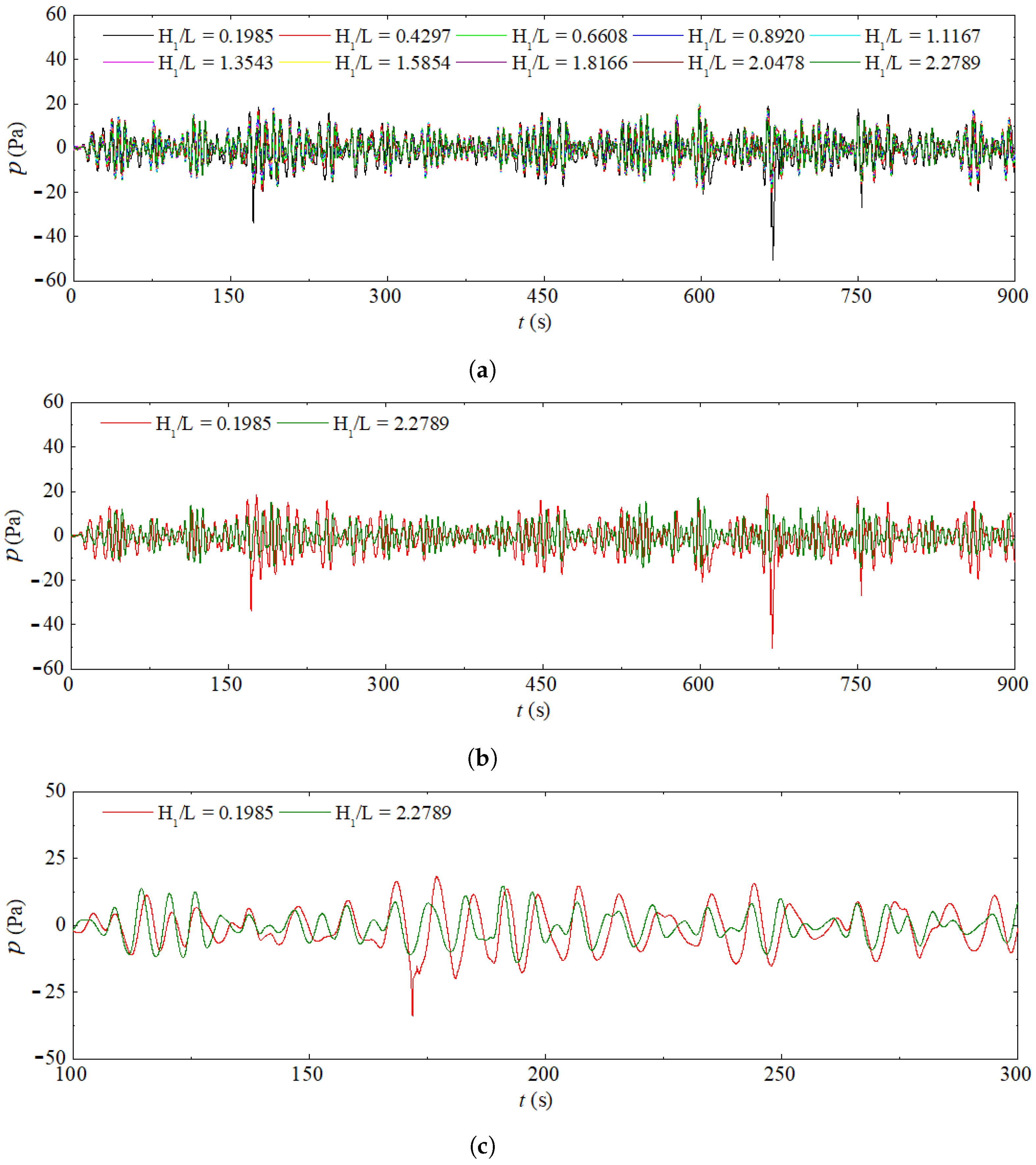
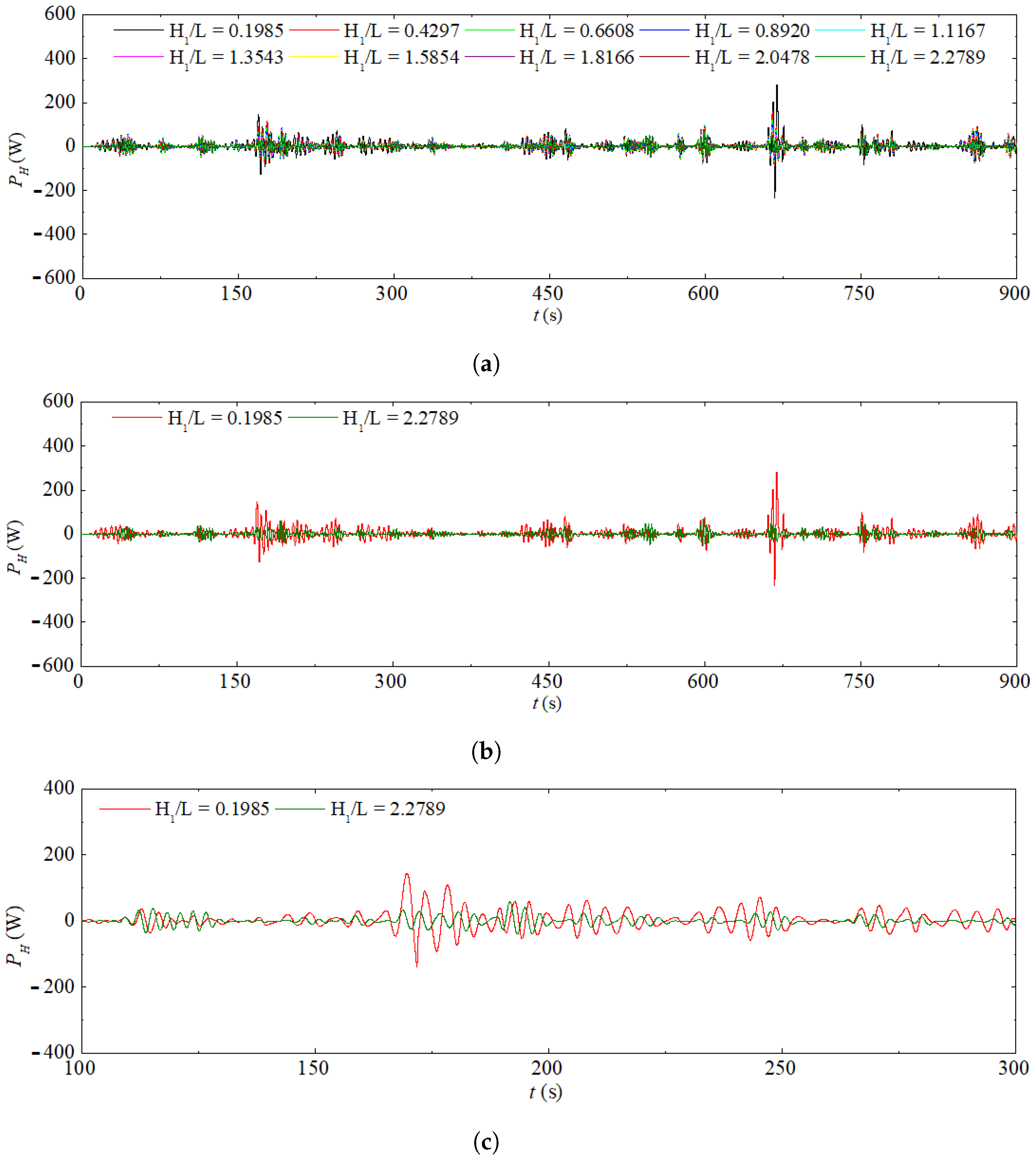
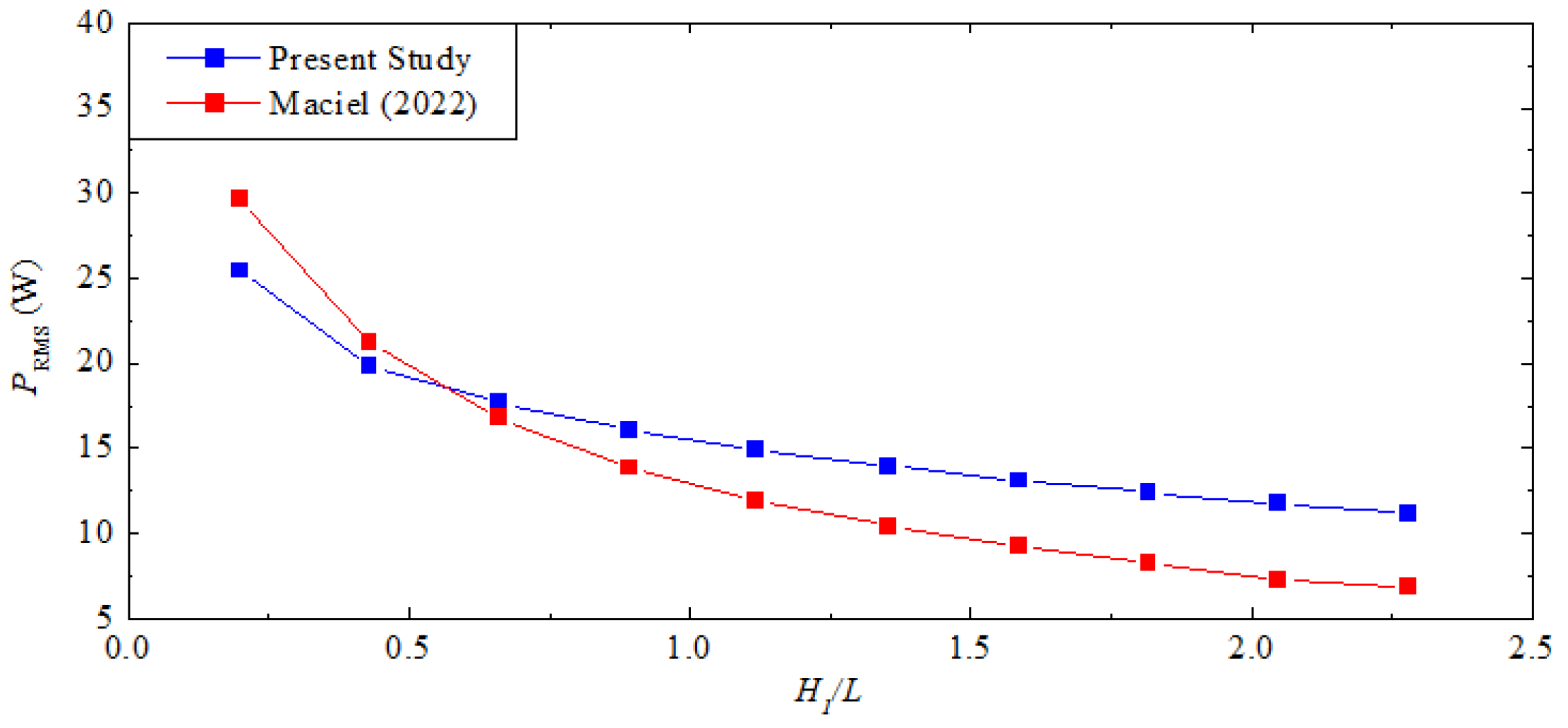
3.2. Study of Geometric Optimization of OWC WEC Subjected to Realistic Irregular Waves
4. Conclusions
Author Contributions
Funding
Institutional Review Board Statement
Informed Consent Statement
Data Availability Statement
Acknowledgments
Conflicts of Interest
Abbreviations
| CFD | Computational fluid dynamics |
| FVM | Finite volume method |
| MAE | Mean absolute error |
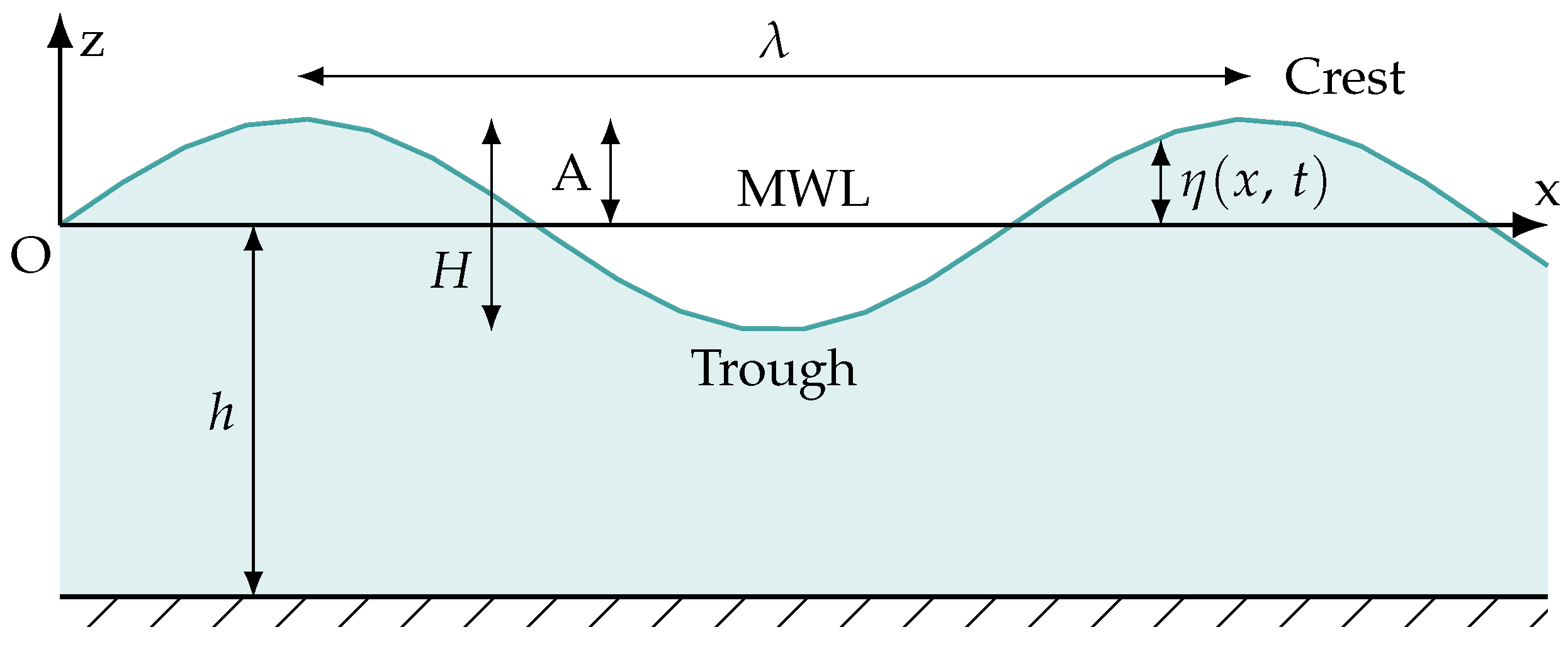
| MWL | Mean water level |
| OWC | Oscillating water column |
| PISO | Pressure-implicit splitting of operators |
| PRESTO | Pressure staggering option |
| RMSE | Root mean square error |
| TOMAWAC | Telemac-based operational model addressing wave action computation |
| VOF | Volume of fluid |
| WEC | Wave energy converter |
| Nomenclature | |
| A | Amplitude of the wave [m] |
| Area of each computational cell volume [m] | |
| Volumetric fraction [–] | |
| Volumetric fraction of air [–] | |
| Volumetric fraction of water [–] | |
| Linear damping coefficient [s] | |
| Quadratic damping coefficient [m] | |
| Time step [s] | |
| Free surface elevation [m] | |
| Gravity acceleration [m/s] | |
| h | Water depth [m] |
| H | Wave height [m] |
| Height of wave channel [m] | |
| Significant height [m] | |
| Height of the hydropneumatic chamber [m] | |
| Height of the turbine duct [m] | |
| Submersion depth of OWC [m] | |
| k | Angular wave number [1/m] |
| L | Length of the hydropneumatic chamber [m] |
| l | Length of the turbine duct [m] |
| Length of the wave channel [m] | |
| Length of the numerical beach [m] | |
| Wavelength [m] | |
| Air mass flow rate [kg/s] | |
| Viscosity [kg/m.s] | |
| n | Number of data [–] |
| Numerical value [–] | |
| p | Static pressure [Pa] |
| Instantaneous available power [W] | |
| Variable field [–] | |
| Air density [kg/m] | |
| Density [kg/m] | |
| Reference value [–] | |
| S | Source term [N/m] |
| Angular wave frequency [Hz] | |
| T | Period [s] |
| Mean period [s] | |
| t | Time [s] |
| Strain rate tensor [N/m] | |
| u | Horizontal velocity [m/s] |
| V | Fluid velocity [m/s] |
| Velocity vector [m/s] | |
| Air velocity in the duct [m/s] | |
| Volume of the hydropneumatic chamber [m] | |
| Total volume of the OWC [m] | |
| w | Vertical velocity [m/s] |
| x | Numerical probe position [m] |
| Starting point [m] | |
| Ending point [m] | |
| Free surface point [m] | |
| Bottom point [m] |
References
- Oliveira, J.F.G.D.; Trindade, T.C.G. Sustainability Performance Evaluation of Renewable Energy Technologies. In Sustainability Performance Evaluation of Renewable Energy Sources: The Case of Brazil; Springer: Berlin/Heidelberg, Germany, 2018. [Google Scholar]
- IPCC. Renewable Energy Sources and Climate Change Mitigation: Special Report of the Intergovernmental Panel on Climate Changel; Cambridge University Press: Cambridge, UK, 2012. [Google Scholar]
- WEC. World Energy Resources; WEC: London, UK, 2016. [Google Scholar]
- Tolmasquim, M.T. Energia Renovável: Hidráulica, Biomassa, Eólica, Solar, Oceânica; Empresa de Pesquisa Energética (EPE): Rio de Janeiro, Brazil, 2006. (In Portuguese) [Google Scholar]
- Khan, N.; Kalair, A.; Abas, N.; Haider, A. Review of ocean tidal, wave and thermal energy technologies. Renew. Sustain. Energy Rev. 2017, 72, 590–604. [Google Scholar] [CrossRef]
- Cruz, J. Ocean Wave Energy: Current Status and Future Prepectives, 1st ed.; Springer: Berlin/Heidelberg, Germany, 2008. [Google Scholar]
- Falcão, A.F.; Henriques, J.C. Oscillating-water-column wave energy converters and air turbines: A review. Renew. Energy 2016, 85, 1391–1424. [Google Scholar] [CrossRef]
- Gomes, M.N. Constructal Design de Dispositivos Conversores de Energia das Ondas do mar em Energia eléTrica do Tipo Coluna de Água Oscilante. Ph.D. Thesis, Universidade Federal do Rio Grande do Sul, Porto Alegre, Brazil, 2014. (In Portuguese). [Google Scholar]
- De Lima, Y.T.B. Análise Geométrica Através do Design Construtal de Conversores de Energia das Ondas do mar do Tipo Coluna de água Oscilante com Câmaras Hidropneumáticas Acopladas. Ph.D. Thesis, Universidade Federal do Rio Grande do Sul, Porto Alegre, Brazil, 2021. (In Portuguese). [Google Scholar]
- Lorenzini, G.; Lara, M.F.E.; Rocha, L.A.O.; Gomes, M.N.; dos Santos, E.D.; Isoldi, L.A. Constructal design applied to the study of the geometry and submergence of an oscillating water column. Int. J. Heat Technol. 2015, 33, 31–38. [Google Scholar] [CrossRef]
- De Lima, Y.T.B.; Rocha, L.A.O.; Gomes, M.N.; dos Santos, E.D. Aplicação Do Método Design Construtal Na Avaliação Numérica Da Potência Hidropneumática De Um Dispositivo Conversor De Energia Das Ondas Do Mar Do Tipo Coluna De Água Oscilante Com Região De Transição Trapezoidal. Rev. Bras. Energias Renov. 2017, 6, 376–396. (In Portuguese) [Google Scholar] [CrossRef]
- De Lima, Y.T.B.; Gomes, M.N.; Cardozo, C.F.; Isoldi, L.A.; dos Santos, E.D.; Rocha, L.A.O. Analysis of geometric variation of three degrees of freedom through the constructal design method for a oscillating water column device with double hidropneumatic chamber. Defect Diffus. Forum 2019, 396, 22–31. [Google Scholar] [CrossRef]
- De Deus, M.J.; Souza, L.C.; Da Silva, M.O.A.; Do Amaral, C.H.A.P.; Dos Santos, E.D.; Isoldi, L.A.; Gomes, M.N. Aplicação de Design Construtal para a Análise Geométrica de um Dispositivo CAO com Formato de Duplo Trapézio Submetido a um Espectro do Tipo Pierson-Moskowitz. Retec-Rev. Tecnol. 2019, 12, 55–67. (In Portuguese) [Google Scholar]
- Teixeira, P.R.F.; Didier, E. Numerical analysis of the response of an onshore oscillating water column wave energy converter to random waves. Energy 2021, 1, 11919. [Google Scholar] [CrossRef]
- Maciel, R.P. Constructal Design Applied to an Oscillating Water Column Wave Energy Converter Device Subjected to a Realistic Sea State. Master’s Thesis, Universidade Federal do Rio Grande, Porto Alegre, Brazil, 2022. [Google Scholar]
- Mavrakos, A.S.; Konispoliatis, D.N.; Ntouras, D.G.; Papadakis, G.P.; Mavrakos, S.A. Hydrodynamics of Moonpool-Type Floaters: A Theoretical and a CFD Formulation. Energies 2022, 15, 570. [Google Scholar] [CrossRef]
- Zabala, I.; Henriques, J.; Blanco, J.; Gomez, A.; Gato, L.; Bidaguren, I.; Falcão, A.; Amezaga, A.; Gomes, R. Wave-induced real-fluid effects in marine energy converters: Review and application to OWC devices. Energy Rev. 2019, 11, 535–549. [Google Scholar] [CrossRef]
- Gomes, M.N.; dos Santos, E.D.; Isoldi, L.A.; Rocha, L.A.O. Two-Dimensional Geometric Optimization of an OscillatingWater Column Converter of Real Scale. In Proceedings of the 22nd International Congress of Mechanical Engineering, Ribeirão Preto, Brazil, 3–7 November 2013; pp. 3468–3479. [Google Scholar]
- Gomes, M.N.; Rocha, L.A.O.; Waess, K.R.; Isoldi, L.A.; dos Santos, E.D. Modelagem Computacional e Otimização Geométrica 2D com Constructal Design de um Dispositivo do Tipo Coluna de Água Oscilante em Escala Real—Comparação Onshore E Offshore. In Proceedings of the XXXIV Iberian Latin-American Congress on Computational Methods in Engineering, Pirenópolis, Brazil, 10–13 November 2013; pp. 1–20. (In Portuguese). [Google Scholar]
- Martins, J.C.; Fragassa, C.; Goulart, M.M.; dos Santos, E.D.; Isoldi, L.A.; Gomes, M.N.; Rocha, L.A.O. Constructal Design of an Overtopping Wave Energy Converter Incorporated in a Breakwater. J. Mar. Sci. Eng. 2022, 10, 471. [Google Scholar] [CrossRef]
- Seibt, F.M.; Isoldi, L.A.; dos Santos, E.D.; Rocha, L.A.O. Study of the Effect of the Relative Height on the Efficiency of a Submerged Horizontal Plate Type Wave Energy Converter Applying Constructal Design. In Proceedings of the XXXVIII Iberian Latin American Congress on Computational Methods in Engineering, Florianópolis, Brazil, 5–8 November 2017. [Google Scholar]
- Bejan, A. Shape and Structure, from Engineering to Nature; Cambridge University Press: Cambridge, UK, 2000. [Google Scholar]
- Pecher, A.; Kofoed, J.P. Handbook of Ocean Wave Energy; Springer: Berlin/Heidelberg, Germany, 2017. [Google Scholar]
- Mahnamfar, F.; Altunkaynak, A. Comparison of numerical and experimental analyses for optimizing the geometry of OWC systems. Ocean. Eng. 2017, 130, 10–24. [Google Scholar] [CrossRef]
- Liu, Z.; Cui, Y.; Xu, C.; Sun, L.; Li, M.; Jin, J. Experimental and numerical studies on an OWC axial-flow impulse turbine in reciprocating air flows. Renew. Sustain. Energy Rev. 2019, 113, 109272. [Google Scholar] [CrossRef]
- Gomes, M.N.; de Deus, M.J.; dos Santos, E.D.; Isoldi, L.A.; Rocha, L.A.O. Analysis of the Geometric Constraints Employed in Constructal Design for Oscillating Water Column Devices Submitted to the Wave Spectrum Through a Numerical Approach. Defect Diffus. Forum 2019, 390, 193–210. [Google Scholar] [CrossRef]
- Dean, R.G.; Dalrymple, R.A. Water Wave Mechanics for Engineers and Scientists; World Scientific: Singapore, 1991. [Google Scholar]
- ANSYS Inc. Ansys Fluent Theory Guide; ANSYS, Inc.: Cannonsburg, PA, USA, 2013. [Google Scholar]
- Hirt, C.W.; Nichols, B.D. Volume of Fluid (VOF) Method for the Dynamics of Free Boundaries. J. Comput. Phys. 1981, 39, 201–225. [Google Scholar] [CrossRef]
- Versteeg, H.K.; Malalasekera, W. An Introduction to Computational Fluid Dynamics—The Finite Volume Method; Pearson Education Limited: London, UK, 2007. [Google Scholar]
- Srinivasan, V.; Salazar, A.J.; Saito, K. Modeling the disintegration of modulated liquid jets using volume-of-fluid (VOF) methodology. Appl. Math. Model. 2011, 35, 3710–3730. [Google Scholar] [CrossRef]
- Cisco, L.A.; Maciel, R.P.; Oleinik, P.H.; dos Santos, E.D.; Gomes, M.N.; Rocha, L.A.O.; Isoldi, L.A.; Machado, B.N. Numerical Analysis of the Available Power in an Overtopping Wave Energy Converter Subjected to a Sea State of the Coastal Region of Tramandaí, Brazil. Fluids 2022, 7, 359. [Google Scholar] [CrossRef]
- Machado, B.N.; Oleinik, P.H.; Kirinus, E.P.; dos Santos, E.D.; Rocha, L.A.O.; Gomes, M.N.; Conde, J.M.P.; Isoldi, L.A. WaveMIMO Methodology: Numerical Wave Generation of a Realistic Sea State. J. Appl. Comput. Mech. 2021, 7, 2129–2148. [Google Scholar] [CrossRef]
- Maciel, R.P.; Fragassa, C.; Machado, B.N.; Rocha, L.A.O.; dos Santos, E.D.; Gomes, M.N.; Isoldi, L.A. Verification and Validation of a Methodology to Numerically Generate Waves Using Transient Discrete Data as Prescribed Velocity Boundary Condition. J. Mar. Sci. Eng. 2021, 9, 896. [Google Scholar] [CrossRef]
- Oleinik, P.H.; Tavares, G.P.; Machado, B.N.; Isoldi, L.A. Transformation of Water Wave Spectra into Time Series of Surface Elevation. Earth 2021, 2, 997–1005. [Google Scholar] [CrossRef]
- Directorate of Hydrography and Navigation of the Brazilian Navy. Nautical Charts|Navy Hydrography Center. Available online: https://www.marinha.mil.br/chm/dados-do-segnav-cartas-nauticas. (accessed on 1 December 2022).
- Cardoso, S.D.; Marques, W.C.; Kirinus, E.d.P.; Stringari, C.E. Levantamento batimétrico usando cartas náuticas. In Proceedings of the 13ª Mostra da Produção Universitária, Rio Grande: Universidade Federal do Rio Grande, Rio Grande, Brazil, 14 October 2014; p. 2. (In Portuguese). [Google Scholar]
- Gomes, M.N.; Nascimento, C.D.; Bonafini, B.L.; dos Santos, E.D.; Isoldi, L.A.; Rocha, L.A.O. Two-dimensional geometric optimization of an oscillating water column converter in laboratory scale. Rev. Eng. Térmica 2012, 11, 30–36. [Google Scholar] [CrossRef]
- Lisboa, R.C.; Teixeira, P.R.; Didier, E. Regular and irregular wave propagation analysis in a flume with numerical beach using a Navier-Stokes based model. Defect Diffus. Forum 2017, 372, 81–90. [Google Scholar] [CrossRef]
- Gomes, M.N.; Isoldi, L.A.; dos Santos, E.D.; Rocha, L.A.O. Análise de malhas para geração numérica de ondas em tanques. In Proceedings of the Anais do VII do Congresso Nacional de Engenharia Mecânica, Associação Brasileira de Engenharia e Ciências Mecânicas, Rio de Janeiro, Brazil, 31 July–3 August 2012. (In Portuguese). [Google Scholar]
- Gomes, M.N.; Lorenzini, G.; Rocha, L.A.O.; dos Santos, E.D.; Isoldi, L.A. Constructal Design Applied to the Geometric Evaluation of an Oscillating Water Column Wave Energy Converter Considering Different Real Scale Wave Periods. J. Eng. Thermophys. 2018, 27, 173–190. [Google Scholar] [CrossRef]
- Letzow, M.; Lorenzini, G.; Barbosa, D.V.E.; Hubner, R.G.; Rocha, L.A.O.; Gomes, M.N.; Isoldi, L.A.; dos Santos, E.D. Numerical Analysis of the Influence of Geometry on a Large Scale Onshore Oscillating Water Column Device with Associated Seabed Ramp. Int. J. Des. Nat. Ecodyn. 2020, 15, 873–884. [Google Scholar] [CrossRef]
- Lima, Y.T.B.; Gomes, M.N.; Isoldi, L.A.; dos Santos, E.D.; Lorenzini, G.; Rocha, L.A.O. Geometric Analysis through the Constructal Design of a Sea Wave Energy Converter with Several Coupled Hydropneumatic Chambers Considering the Oscillating Water Column Operating Principle. Appl. Sci. 2021, 11, 8630. [Google Scholar] [CrossRef]
- Chai, T.; Draxler, R.R. Root mean square error (RMSE) or mean absolute error (MAE)? – Arguments against avoiding RMSE in the literature. Geosci. Model Dev. 2014, 7, 1247–1250. [Google Scholar] [CrossRef]
- Dizadji, N.; Sajadian, S.E. Modeling and optimization of the chamber of OWC system. Energy 2011, 36, 2360–2366. [Google Scholar] [CrossRef]
- Holthuijsen, L.H. Waves in Oceanic and Coastal Waters; Cambridge University Press: Cambridge, UK, 2007. [Google Scholar]
- Strauch, J.C.; Cuchiara, D.C.; Toldo, E.E., Jr.; Almeida, L.E.S.B. O padrão das ondas de verão e outono no litoral sul e norte do Rio Grande do Sul. Rev. Bras. Recur. Hídricos 2009, 14, 29–37. (In Portuguese) [Google Scholar] [CrossRef]


| (m) | L (m) | |
|---|---|---|
| 0.1985 | 5.65 | 28.46 |
| 0.4297 | 8.31 | 19.34 |
| 0.6608 | 10.31 | 15.16 |
| 0.8920 | 11.98 | 13.43 |
| 1.1167 | 13.40 | 12.00 |
| 1.3543 | 14.76 | 10.90 |
| 1.5854 | 15.97 | 10.07 |
| 1.8166 | 17.09 | 9.41 |
| 2.0478 | 18.15 | 8.86 |
| 2.2789 | 19.14 | 8.40 |
| Probe Position (m) | MAE (m) | RMSE (m) |
|---|---|---|
| 0.000000 | 0.004264 | 0.006133 |
| 10.455425 | 0.019815 | 0.020653 |
| 20.910851 | 0.019803 | 0.020501 |
| 31.366276 | 0.019803 | 0.020468 |
| 41.821702 | 0.019835 | 0.020556 |
| 50.186042 | 0.019836 | 0.020555 |
| 60.641468 | 0.019802 | 0.020494 |
| 71.096893 | 0.019757 | 0.020514 |
| 81.552318 | 0.019746 | 0.020618 |
| 92.007744 | 0.019743 | 0.020814 |
| 102.463169 | 0.019682 | 0.021028 |
Disclaimer/Publisher’s Note: The statements, opinions and data contained in all publications are solely those of the individual author(s) and contributor(s) and not of MDPI and/or the editor(s). MDPI and/or the editor(s) disclaim responsibility for any injury to people or property resulting from any ideas, methods, instructions or products referred to in the content. |
© 2023 by the authors. Licensee MDPI, Basel, Switzerland. This article is an open access article distributed under the terms and conditions of the Creative Commons Attribution (CC BY) license (https://creativecommons.org/licenses/by/4.0/).
Share and Cite
Mocellin, A.P.G.; Maciel, R.P.; Oleinik, P.H.; dos Santos, E.D.; Rocha, L.A.O.; Ziebell, J.S.; Isoldi, L.A.; Machado, B.N. Geometrical Analysis of an Oscillating Water Column Converter Device Considering Realistic Irregular Wave Generation with Bathymetry. J. Exp. Theor. Anal. 2023, 1, 24-43. https://doi.org/10.3390/jeta1010003
Mocellin APG, Maciel RP, Oleinik PH, dos Santos ED, Rocha LAO, Ziebell JS, Isoldi LA, Machado BN. Geometrical Analysis of an Oscillating Water Column Converter Device Considering Realistic Irregular Wave Generation with Bathymetry. Journal of Experimental and Theoretical Analyses. 2023; 1(1):24-43. https://doi.org/10.3390/jeta1010003
Chicago/Turabian StyleMocellin, Ana Paula Giussani, Rafael Pereira Maciel, Phelype Haron Oleinik, Elizaldo Domingues dos Santos, Luiz Alberto Oliveira Rocha, Juliana Sartori Ziebell, Liércio André Isoldi, and Bianca Neves Machado. 2023. "Geometrical Analysis of an Oscillating Water Column Converter Device Considering Realistic Irregular Wave Generation with Bathymetry" Journal of Experimental and Theoretical Analyses 1, no. 1: 24-43. https://doi.org/10.3390/jeta1010003