
Relating the Ramsay Quotient Model to the Classical D-Scoring Rule

1
IPN—Leibniz Institute for Science and Mathematics Education, Olshausenstraße 62, 24118 Kiel, Germany
2
Centre for International Student Assessment (ZIB), Olshausenstraße 62, 24118 Kiel, Germany
Analytics 2023, 2(4), 824-835; https://doi.org/10.3390/analytics2040043
Submission received: 27 August 2023
/
Revised: 4 October 2023
/
Accepted: 9 October 2023
/
Published: 17 October 2023
Abstract
:In a series of papers, Dimitrov suggested the classical D-scoring rule for scoring items that give difficult items a higher weight while easier items receive a lower weight. The latent D-scoring model has been proposed to serve as a latent mirror of the classical D-scoring model. However, the item weights implied by this latent D-scoring model are typically only weakly related to the weights in the classical D-scoring model. To this end, this article proposes an alternative item response model, the modified Ramsay quotient model, that is better-suited as a latent mirror of the classical D-scoring model. The reasoning is based on analytical arguments and numerical illustrations.
1. Introduction
Item response theory (IRT; [1]) is the statistical analysis of test items in education, psychology, and other fields of social sciences. Typically, a number of test items are administered to test-takers. The primary interest lies in inferring the ability (performance or trait) based on the test items. IRT models relate observed item responses to unobserved latent traits. Because the latent trait is unobserved, there are many plausible choices for modeling these relationships. The most popular class of IRT models is that of logistic IRT models [2].
Recently, in a series of papers and a well-written summary book, the researcher Dimiter Dimitrov [3,4] suggested the classical D-scoring rule for scoring items that gives difficult items a higher weight while easier items receive a lower weight. Subsequently, the so-called latent D-scoring model has been proposed as a latent analog of the classical D-scoring model [5]. However, it has been shown that this proposed model is statistically equivalent to the widely used two-parameter logistic IRT model [6]. As argued later in this article, the weights implied by this latent D-scoring model are far from perfectly related to the weights in the classical D-scoring model. This article proposes an alternative IRT model, a modified Ramsay quotient model, that can be interpreted as a latent analog ([3]; or a latent mirror, [4]) of the classical D-scoring rule. The usefulness of the Ramsay quotient model is demonstrated based on analytical and numerical arguments.
The remainder of the article is organized as follows. Section 2 briefly reviews IRT models. In particular, it focuses on the two-parameter logistic and the Ramsay quotient model. Section 3 reviews the classical and latent D-scoring model of Dimitrov. In Section 4, a variant of the Ramsay quotient model is proposed intended to serve as an adequate latent D-scoring model. The usefulness of this model is illustrated in Section 5 using five empirical datasets. Finally, the article closes with a discussion in Section 6.
2. Item Response Modeling
Let be a vector of I binary random variables () that are also referred to as items or item responses. A unidimensional IRT model [2,7,8] model parametrizes the multivariate distribution for as
where F is the distribution function of the latent trait (also referred to as the ability variable) that depends on a parameter . The quantity is referred to as the item response function (IRF) for item i that depends on a parameter . From (1), it can be seen that items are conditionally independent given the latent trait . Some identification constraints on item parameters or distribution parameters must be imposed to ensure model identification [9].
If the IRT model (1) has been estimated, individual ability estimates can be estimated by maximizing the log-likelihood function l that gives the most likely ability estimate for given a vector of item responses . The log-likelihood function is given by (see [1])
By taking the derivative with respect to in (2), the ability estimate fulfills the nonlinear equation
where .
Most IRT models take the full item response pattern into account [10,11,12]. It is only for the simple Rasch model (RM, [13], see Section 2.1.1) that the sum score is a sufficient statistic, and not every item response pattern results in a different ability score.
2.1. Two-Parameter Logistic (2PL) Item Response Model
An important class of IRT models is the class of logistic IRT models. Logistic IRT models employ the logistic link function for parameterizing IRFs. The IRFs in the two-parameter logistic (2PL) model [14] are given by
where denotes item discriminations and denotes item difficulties. The ability variable is typically real-valued. Frequently, a normal distribution is chosen in the 2PL model. However, this assumption can be weakened [15].
An important (and well-known) property of the 2PL model is that is a sufficient statistic for [2]. This directly follows because the individual log-likelihood function defined in (2) can be derived as
A frequently employed identification constraint in the 2PL model is and var. Alternatively, the item discrimination and the item difficulty for one item can be fixed; that is, and for some .
2.1.1. Rasch Model (1PL Model)
The one-parameter logistic (1PL) model (RM; [13]) is obtained by setting all item discriminations in the 2PL model equal to one (i.e., for ). In this case, the IRF is given by
Note that, in (6), a difference between the ability and the item difficulty is involved. Therefore, the model could also be referred to as the Rasch difference model. Note that is a sufficient statistic for in the RM.
In the RM, = 0 is a frequently utilized identification constraint. Alternatively, one item difficulty could be set to zero. As a further alternative, the mean of the item difficulties could be set to zero.
2.1.2. Implementation
The 1PL model or the 2PL model can be estimated using marginal maximum likelihood (MML) using an expectation–maximization (EM) algorithm [16]. Alternatively, the estimation could be carried out using Newton–Raphson algorithms. More generally, the R [17] packages mirt [18] (using the function mirt::mirt() in combination with mirt::createItem() and mirt::createGroup() or sirt [19] (using the function sirt::xxirt()) allow users to arbitrarily define IRFs () and distribution functions F in the IRT model (1) that should be estimated.
2.2. Ramsay Quotient Model (RQM)
Ramsay [20] proposed a quotient of a positive ability variable and a positive item difficulty parameter in their quotient model as an alternative to the difference model of Rasch (see (6)). The IRF in the Ramsay quotient model (RQM; [20]) is defined as
Note that the positive item parameter also allows the representation of guessing effects in multiple-choice items [20]. It should be emphasized that the RQM can be rewritten (7) as (see [20])
which corresponds to a 2PL model with a positively valued ability. The item discrimination and the item difficulty are given by and , respectively. Interestingly, the item discrimination is necessarily correlated with item difficulty. Also, note that is a sufficient statistic for the latent ability because (8) is a 2PL model. An interesting model might result in constraining equal across items (i.e., for all ). Then, the implied item discrimination is indirectly proportional to the item difficulty . That is, we get .
To sum up, the RQM is a particularly constrained 2PL model with a positively valued ability variable . The item difficulty from the RQM enters both item discrimination and item difficulty from the 2PL model. Interestingly, the RQM is related to the diffusion model of Ratcliffe that is utilized in cognitive psychology for modeling response times [21,22]. Furthermore, the RQM shares the simplicity of the Rasch model if used with only one item parameter but provides a simple alternative to handle guessing effects. In contrast to the three-parameter logistic IRT model, a linearly weighted statistic of items for the latent ability is available for the RQM.
Implementation
To estimate the RQM defined by the IRFs in (7), it is convenient to define and . These parameters are unbounded in contrast to the original definition in the RQM. If a normal distribution for is assumed, there is a log-normal distribution for results. The IRF in (8) can then be written as
Using the last term on the right side of Equation (9) is preferable to avoid numerical overflow.
3. Dimitrov’s D-Scoring Approach
3.1. Classical D-Scoring Method
The classical D-scoring approach was proposed by Dimitrov [3]. Based on I observed binary item responses (), the classical D-score is defined as
The variable is a weighted sum score in which the weights are given as one minus the p-value of one item. Hence, difficult items are upweighted, and easy items are downweighted in the scoring rule (10). Such a rationale for scoring items might be appealing to some practitioners. Of course, it might be reasonable in a high-stakes test to inform test takers before the test administration when implementing such an unconventional scoring rule [23].
3.2. Rational Function Model (RFM) as a Latent D-Scoring Model
Dimitrov and Atanasov [5] (see also [24]) propose an IRT model, the latent D-scoring method that “can be seen as a latent analog to the classical” D-scoring method ([4], p. 64) described in Section 3.1 (see (10)). The model is called the rational function model (RFM), and the IRF for item is defined by
where is the latent ability variable taking values between 0 and 1. The parameter (with ) can be interpreted as a difficulty parameter in the RFM, and is a positive shape parameter. Robitzsch [6] pointed out that the RFM is equivalent to the 2PL model (4) by defining the transformed parameters
Hence, the estimation of the RFM can be carried out using software for the 2PL model [6]. The only ambiguity is about specifying the distribution of the latent variable . If an identification constraint is defined for an item (e.g., and ), sufficiently flexible distributions for can be estimated, given the distribution parameters can be empirically identified. The density function of can be obtained using a density transformation of (see Equation (12) in [6]).
As pointed out in [4] (Ch. 12), and are typically highly correlated in empirical applications (e.g., ), although the ability estimators are nonlinearly (but monotonically) related.
Dimitrov ([4], p. xiv) claimed that the latent D-score variable “is a latent mirror” of the classical D-score , “with some advantages in the accuracy of estimation” ([4], p. xiv). The authors computed the ability estimates and correlated them with . In a real-data example involving an English proficiency test with 100 items administered by the National Center for Assessment in Saudi Arabia, the correlation was 0.974. It was argued that this correlation was still high enough to demonstrate that the classical D-score is a good proxy of the latent D-score [4,5]. We tend to disagree with this reasoning. First, reasonably different IRT models will typically lead to high correlations between their ability estimates, questioning the usefulness of this measure. Second, it is clear that the two scores will differ because they involve different weighting schemes. In the classical D-score , items are weighted by item difficulty in the sufficient statistic , while the ability estimate as a nonlinear transformation of the ability estimate from the 2PL model possesses the sufficient statistic . Hence, the correlation between and will be primarily a function of the correlation of the weights and () across items. An obvious latent mirror of the classical D-scoring rule is obtained if the 2PL model would be estimated with fixed item discriminations (as can also be seen in [25]). Then, the sum score would necessarily be a sufficient statistic of the ability . In the 2PL model with fixed item discriminations, the standard deviation of can be freely estimated.
4. Modified Ramsay Quotient Model and the Classical D-Scoring Rule
In this section, we present an IRT model that directly implements the idea that more difficult items should receive a higher score in the latent variable.
The RQM has the attractive property that it is equivalent to a particular 2PL model (see Section 2.2) in which the difficulty of an item is simultaneously reflected in the item discrimination and the item difficulty parameters. However, the RQM defined in (8) implies that more difficult items (i.e., with a larger ) become downweighted in terms of item discrimination (i.e., becomes smaller). This is the converse of what is defined in the classical D-score in (10). In the classical D-score computation, more difficult items receive a higher weight.
Nevertheless, one could simply swap the roles of correct and incorrect item responses in the RQM. We apply the RQM from (7) and (9) and define the IRF for an incorrect item response
where and . Note that the term “” appears in (13) because the newly defined latent variable should reflect its ability instead of its non-ability, which is parametrized when modeling incorrect item responses (i.e., ) with the RQM. Also, note that we constrained all K parameters to be equal across items in (13) in order to maximally reflect the item difficulty in the item parameter (and ). Note that the probability of a correct item response is given as
According to the 2PL parametrization of the RQM in (8), the IRF in (13) can be written as
Consequently, is a sufficient statistic for , , or any injective transformation of . Trivially, is also a sufficient statistic for these variables. Because incorrect item responses were applied in the RQM, reflects item easiness. Hence, easy items get downweighted in this sufficient statistic (and therefore in and their monotone transformations). This is the desired property in the classical D-scoring approach.
The application of this variant of the RQM also depends on the joint K item parameter. Of course, one can simultaneously estimate all item parameters () and the variance of in the modified RQM. However, the fit of the IRT model will typically be a function of K. Because our goal is to make the modified RQM maximally equivalent to the classical D-scoring approach, we repeatedly fit the modified RQM on grid values of K (say, from to 100). Then, we choose the model whose associations in estimated weights from the modified RQM in (15) and the weights are maximal (see the next Section 5).
5. Numerical Examples
We tested our newly proposed latent D-scoring approach based on the modified RQM (see Section 4) with the classical D-scoring approach discussed in Section 3.1 for several datasets containing binary item responses. For each of the datasets, we fitted the RQM assuming a normal distribution for the latent variable with a fixed mean of 0, and we estimated the standard deviation (SD) of . We also estimated the difficulty parameter on the log scale, meaning that was estimated, and the parameter was computed as .
For each dataset, we estimated the modified RQM for a fixed K parameter for . Then, we fitted a linear regression model through the origin according to the model
where are the weights used in the classical D-score . Based on the linear regression (16), we computed the determination coefficient that quantifies how well the weights were approximated by the weights obtained from the modified RQM as the latent D-scoring model. Because is a function of K, the optimal RQM that is intended to be used for latent D-scoring can be chosen with the corresponding K that maximizes the determination coefficient .
We also specified a linear regression model of weights on item discriminations from the 2PL model to assess the similarity of the classical D-scoring rule with the scores from the latent D-scoring model by means of the determination coefficient . The regression model was given by
In order to compare the implications of the different weights from the models, we computed correlations of the classical D-score with linearly weighted item scores, where the weights were obtained from the RQM (i.e., the RQM D-score) and the 2PL model (i.e., the latent D-score), respectively.
All analyses were carried out in the R software (Version 4.3.1, [17]). The estimation of the modified RQM utilized the sirt::xxirt() function in the R package sirt [19]. The R code for model specification can be found at https://osf.io/nrcag (accessed on 26 September 2023).
In the following, results from five publicly available binary item response datasets were reported. All datasets had no missing values.
The first dataset data.si06 from the R package sirt [19] contains 4441 students on 14 items. The data stem from a verbal comprehension test. Figure 1 displays the determination coefficient of the regression (16) of the weights of the classical D-score on the weights obtained from the modified RQM as a function of the parameter K. There is a maximum , which is attained at . Figure 2 displays the weights on the y axis and the weights on the x axis for the optimal value . The estimated SD of from the RQM was 0.459. In addition, the fitted regression line from (16) is shown in Figure 2. It can be seen that the obtained of 0.997 implies that weights from the classical D-score were well predicted by weights from the RQM.
Figure 3 includes the regression (17) of weights on the estimated weights from the 2PL model. It can be seen that the weights from the classical D-scoring rule are not well predicted by weights estimated in the 2PL model. The determination coefficient from the regression model was only .
The classical D-score was correlated with the RQM score at 0.9995, while the correlation with the 2PL score was much lower at 0.9072.
Table 1 contains estimated item parameters from the RQM with and the 2PL model. In this table, normalized item weights for the sufficient statistics of the different scores were computed that have an average weight of 1. It can be seen that normalized weights based on the RQM and the parameters from classical D-scoring were very similar. However, these weights substantially differed from the weights obtained from the 2PL model, which are also displayed in Figure 3.
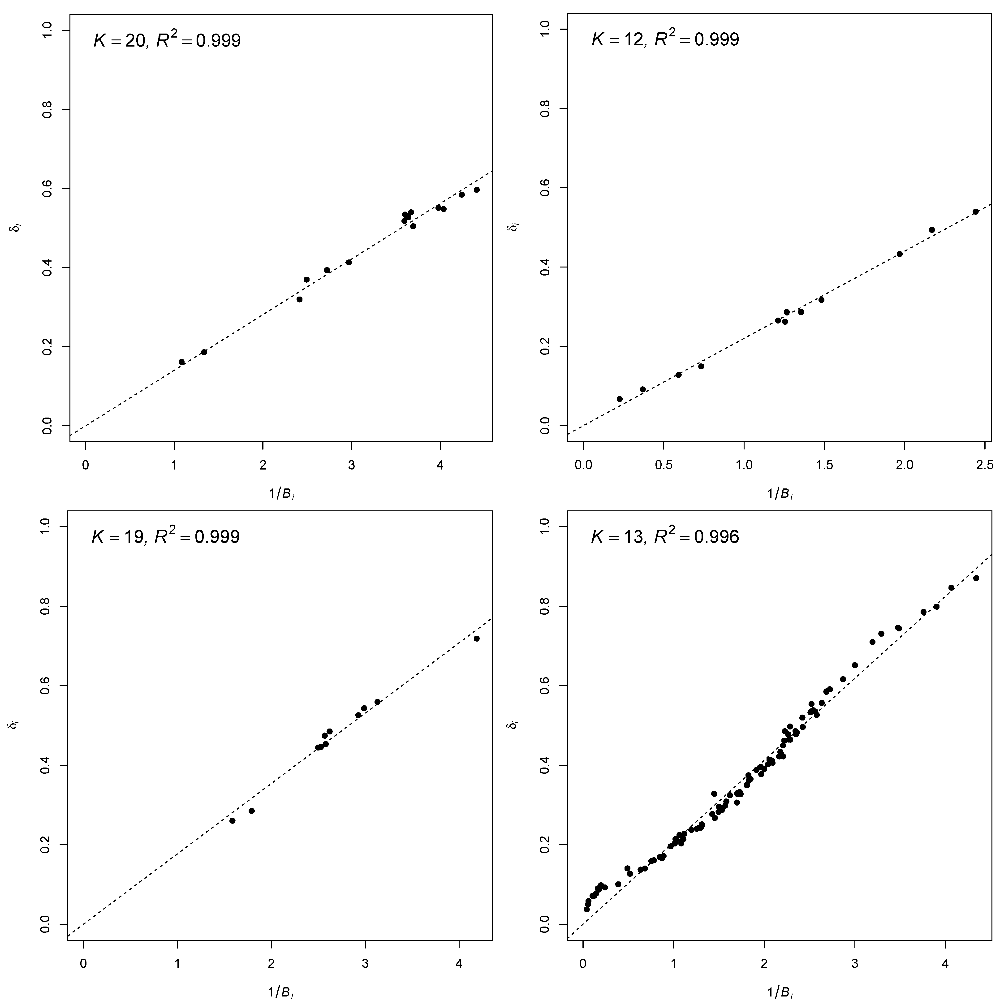
The second dataset data.numeracy can be found in the R package TAM [26]. It contains 876 students on 15 items. The data resulted from a numerical comprehension test. The upper left panel in Figure 4 displays the determination coefficient of the regression (16) of the weights of the classical D-score on the weights obtained from the modified RQM. The estimated SD of from the RQM was 0.505. The maximum value of 0.999 was attained for . It can be seen in the upper left panel in Figure 4 that the weights from the classical D-score were almost perfectly predicted by weights from the RQM. The determination coefficient from the regression model of weights from classical D-scoring onto weights from the 2PL model was . The classical D-score correlated with the RQM score at 0.9999, while the correlation with the 2PL score was much lower at 0.9909.
The third dataset data.read from the R package sirt contains 328 students on 12 items. It stems from a reading comprehension test involving three reading comprehension text stimuli. Like in the first dataset, weights from the classical D-score were satisfactorily predicted by the weights from the RQM as indicated by the of 0.999 (see the upper-right panel in Figure 4). The optimal K regarding the maximum determination coefficient was . The estimated SD of from the RQM was 0.519. The determination coefficient from the regression model of weights from classical D-scoring onto weights from the 2PL model was . The classical D-score correlated with the RQM score at 0.9998, while the correlation with the 2PL score was much lower at 0.8742.
The fourth dataset data.pisaMath from the sirt package contains 565 students on 11 items. The data resulted from a PISA mathematics test involving Austrian students. As the lower-left panel in Figure 4 indicates, the weights of the classical D-score were well predicted () by the weights from the modified RQM for the optimal . The estimated SD of from the RQM was 0.433. The determination coefficient from the regression model of weights from classical D-scoring onto weights from the 2PL model was . The classical D-score correlated with the RQM score at 0.9999, while the correlation with the 2PL score was much lower at 0.9938.
Finally, the fifth dataset Psych101 from the KernSmoothIRT [27,28] package contains 379 students on 100 items. The data stem from an exam from a psychology class. The lower-right panel in Figure 4 shows some notable deviations from the regression line, and the determination coefficient was 0.996 for the optimal value of . The estimated SD of from the RQM was 0.246. The determination coefficient from the regression model of weights from classical D-scoring onto weights from the 2PL model was . The classical D-score correlated with the RQM score at 0.9997, while the correlation with the 2PL score was much lower at 0.9551.
It can be shown that item weights are a nonlinear function of 2PL item parameters and [29]. Therefore, an anonymous reviewer argued that a low correlation between and is expected. We agree with such a view. However, such an observation questions the view of why one should ever believe that the classical D-score approximates the latent D-score (or the other way around).
It was pointed out by an anonymous reviewer that the correlations between the classical D-scores and the 2PL scores (i.e., latent D-score) were quite high because they ranged between 0.9072 and 0.9938, with the exception of the third dataset () that had the smallest number of items. However, we disagree with the anonymous reviewer that these correlation sizes would imply that classical and latent D-scores provide similar findings. In contrast, the item weights implied by the different scoring rules are only weakly related.
6. Discussion
This article searched for an IRT model that follows the principle of classical D-scoring of Dimitrov. In this approach, more difficult items receive higher weights in the classical D-score, which is a weighted sum score. It was shown that a variant of the RQM proves useful in this regard. In the RQM, a weighted sum score is a sufficient statistic for the latent variable contained in this model. Furthermore, in our proposed model, more difficult items are strongly weighted in the sum score. We demonstrated the adequacy of the RQM through five example datasets. Because the weights in the classical D-score were very well predicted by weights obtained from the RQM, one can interpret the RQM as a latent mirror of the D-scoring model. Although the weights were not perfectly predicted in all datasets, one can at least say that the RQM serves as a much more appropriate latent analog of the classical D-scoring model than the latent D-scoring model originally proposed by Dimitrov.
The classical and latent D-scoring methods were applied to important fields in educational measurement. Research was conducted in the areas of differential item functioning [30], test equating and linking [31], multistage testing [32], and standard setting [33]. The proposed methodology can be compared in future research with appropriate adaptations that involve the Ramsay quotient model.
Funding
This research received no external funding.
Informed Consent Statement
Informed consent was obtained from all subjects involved in the study.
Data Availability Statement
The datasets used in this article are available in R packages (see Section 5).
Acknowledgments
The author would like to thank Dimiter Dimitrov, three anonymous reviewers, and the academic editor for their helpful comments and suggestions that helped improve the paper.
Conflicts of Interest
The author declares no conflict of interest.
Abbreviations
The following abbreviations are used in this manuscript:
| 1PL | one-parameter logistic |
| 2PL | two-parameter logistic |
| CTT | classical test theory |
| EM | expectation maximization |
| IRF | item response function |
| IRT | item response theory |
| RFM | rational function model |
| RM | Rasch model |
| RQM | Ramsay quotient model |
| SD | standard deviation |
References
- Baker, F.B.; Kim, S.H. Item Response Theory: Parameter Estimation Techniques; CRC Press: Boca Raton, FL, USA, 2004. [Google Scholar] [CrossRef]
- Yen, W.M.; Fitzpatrick, A.R. Item response theory. In Educational Measurement; Brennan, R.L., Ed.; Praeger Publishers: Westport, CT, USA, 2006; pp. 111–154. [Google Scholar]
- Dimitrov, D.M. An approach to scoring and equating tests with binary items: Piloting with large-scale assessments. Educ. Psychol. Meas. 2016, 76, 954–975. [Google Scholar] [CrossRef] [PubMed]
- Dimitrov, D. D-scoring Method of Measurement: Classical and Latent Frameworks; Taylor & Francis: Boca Raton, FL, USA, 2023. [Google Scholar] [CrossRef]
- Dimitrov, D.M.; Atanasov, D.V. Latent D-scoring modeling: Estimation of item and person parameters. Educ. Psychol. Meas. 2021, 81, 388–404. [Google Scholar] [CrossRef]
- Robitzsch, A. About the equivalence of the latent D-scoring model and the two-parameter logistic item response model. Mathematics 2021, 9, 1465. [Google Scholar] [CrossRef]
- Chen, Y.; Li, X.; Liu, J.; Ying, Z. Item response theory – A statistical framework for educational and psychological measurement. arXiv 2021, arXiv:2108.08604. [Google Scholar] [CrossRef]
- van der Linden, W.J. Unidimensional logistic response models. In Handbook of Item Response Theory, Volume 1: Models; van der Linden, W.J., Ed.; CRC Press: Boca Raton, FL, USA, 2016; pp. 11–30. [Google Scholar]
- San Martin, E. Identification of item response theory models. In Handbook of Item Response Theory, Volume 2: Statistical Tools; van der Linden, W.J., Ed.; CRC Press: Boca Raton, FL, USA, 2016; pp. 127–150. [Google Scholar] [CrossRef]
- Bock, R.D.; Gibbons, R.D. Item Response Theory; Wiley: New York, NY, USA, 2021. [Google Scholar] [CrossRef]
- da Silva, J.G.; da Silva, J.M.N.; Bispo, L.G.M.; de Souza, D.S.F.; Serafim, R.S.; Torres, M.G.L.; Leite, W.K.d.S.; Vieira, E.M.d.A. Construction of a musculoskeletal discomfort scale for the lower limbs of workers: An analysis using the multigroup item response theory. Int. J. Environ. Res. Public Health 2023, 20, 5307. [Google Scholar] [CrossRef] [PubMed]
- Schmahl, C.; Greffrath, W.; Baumgärtner, U.; Schlereth, T.; Magerl, W.; Philipsen, A.; Lieb, K.; Bohus, M.; Treede, R.D. Differential nociceptive deficits in patients with borderline personality disorder and self-injurious behavior: Laser-evoked potentials, spatial discrimination of noxious stimuli, and pain ratings. Pain 2004, 110, 470–479. [Google Scholar] [CrossRef] [PubMed]
- Rasch, G. Probabilistic Models for Some Intelligence and Attainment Tests; Danish Institute for Educational Research: Copenhagen, Denmark, 1960. [Google Scholar]
- Birnbaum, A. Some latent trait models and their use in inferring an examinee’s ability. In Statistical Theories of Mental Test Scores; Lord, F.M., Novick, M.R., Eds.; MIT Press: Reading, MA, USA, 1968; pp. 397–479. [Google Scholar]
- Xu, X.; von Davier, M. Fitting the Structured General Diagnostic Model to NAEP Data; (Research Report No. RR-08-28); Educational Testing Service: Princeton, NJ, USA, 2008. [Google Scholar] [CrossRef]
- Aitkin, M. Expectation maximization algorithm and extensions. In Handbook of Item Response Theory, Vol. 2: Statistical Tools; van der Linden, W.J., Ed.; CRC Press: Boca Raton, FL, USA, 2016; pp. 217–236. [Google Scholar] [CrossRef]
- R Core Team. R: A Language and Environment for Statistical Computing; R Core Team: Vienna, Austria, 2023; Available online: https://www.R-project.org/ (accessed on 15 March 2023).
- Chalmers, R.P. mirt: A multidimensional item response theory package for the R environment. J. Stat. Softw. 2012, 48, 1–29. [Google Scholar] [CrossRef]
- Robitzsch, A. R Package Version 4.0-6; sirt: Supplementary Item Response Theory Models; R Foundation for Statistical Computing: Vienna, Austria, 2023; Available online: https://github.com/alexanderrobitzsch/sirt (accessed on 12 August 2023).
- Ramsay, J.O. A comparison of three simple test theory models. Psychometrika 1989, 54, 487–499. [Google Scholar] [CrossRef]
- van der Maas, H.L.J.; Molenaar, D.; Maris, G.; Kievit, R.A.; Borsboom, D. Cognitive psychology meets psychometric theory: On the relation between process models for decision making and latent variable models for individual differences. Psychol. Rev. 2011, 118, 339–356. [Google Scholar] [CrossRef] [PubMed]
- Molenaar, D.; Tuerlinckx, F.; van der Maas, H.L.J. Fitting diffusion item response theory models for responses and response times using the R package diffIRT. J. Stat. Softw. 2015, 66, 1–34. [Google Scholar] [CrossRef]
- Hemker, B.T. To a or not to a: On the use of the total score. In Essays on Contemporary Psychometrics; van der Ark, L.A., Emons, W.H.M., Meijer, R.R., Eds.; Springer: Cham, Switzerland, 2023; pp. 251–270. [Google Scholar] [CrossRef]
- Dimitrov, D.M. Modeling of item response functions under the D-scoring method. Educ. Psychol. Meas. 2020, 80, 126–144. [Google Scholar] [CrossRef] [PubMed]
- Verhelst, N.D.; Glas, C.A.W. The one parameter logistic model. In Rasch Models. Foundations, Recent Developments, and Applications; Fischer, G.H., Molenaar, I.W., Eds.; Springer: New York, NY, USA, 1995; pp. 215–237. [Google Scholar] [CrossRef]
- Robitzsch, A.; Kiefer, T.; Wu, M. R Package Version 4.1-4; TAM: Test Analysis Modules; R Foundation for Statistical Computing: Vienna, Austria, 2022; Available online: https://CRAN.R-project.org/package=TAM (accessed on 28 August 2022).
- Mazza, A.; Punzo, A.; McGuire, B. KernSmoothIRT: An R package for kernel smoothing in item response theory. J. Stat. Softw. 2014, 58, 1–34. [Google Scholar] [CrossRef]
- Ramsay, J.O.; Abrahamowicz, M. Binomial regression with monotone splines: A psychometric application. J. Am. Stat. Assoc. 1989, 84, 906–915. [Google Scholar] [CrossRef]
- Dimitrov, D.M. Marginal true-score measures and reliability for binary items as a function of their IRT parameters. Appl. Psychol. Meas. 2003, 27, 440–458. [Google Scholar] [CrossRef]
- Dimitrov, D.M.; Atanasov, D.V. Testing for differential item functioning under the D-scoring method. Educ. Psychol. Meas. 2022, 82, 107–121. [Google Scholar] [CrossRef] [PubMed]
- Dimitrov, D.M.; Atanasov, D.V. An approach to test equating under the latent D-scoring method. Meas. Interdiscip. Res. Persp. 2021, 19, 153–162. [Google Scholar] [CrossRef]
- Han, K.C.T.; Dimitrov, D.M.; Al-Mashary, F. Developing multistage tests using D-scoring method. Educ. Psychol. Meas. 2019, 79, 988–1008. [Google Scholar] [CrossRef] [PubMed]
- Dimitrov, D.M. The response vector for mastery method of standard setting. Educ. Psychol. Meas. 2022, 82, 719–746. [Google Scholar] [CrossRef] [PubMed]
Figure 1.
Dataset data.si06 from R package sirt: Determination coefficient as a function of K for the regression of weights used in classical D-scoring on estimated weights 1/ (see (16)). The red triangle corresponds to the K value with the maximum .
Figure 1.
Dataset data.si06 from R package sirt: Determination coefficient as a function of K for the regression of weights used in classical D-scoring on estimated weights 1/ (see (16)). The red triangle corresponds to the K value with the maximum .

Figure 2.
Dataset data.si06 from R package sirt: Regression of weights used in classical D-scoring on estimated weights 1/ from the RQM with optimal K (see (16)).
Figure 2.
Dataset data.si06 from R package sirt: Regression of weights used in classical D-scoring on estimated weights 1/ from the RQM with optimal K (see (16)).

Figure 3.
Dataset data.si06 from R package sirt: Regression of weights used in classical D-scoring on estimated weights from the 2PL model (see (17)).
Figure 3.
Dataset data.si06 from R package sirt: Regression of weights used in classical D-scoring on estimated weights from the 2PL model (see (17)).

Figure 4.
Regression of weights used in classical D-scoring on estimated weights 1/ from the RQM with optimal K (see (16)). Upper-left panel: dataset data.numeracy from R package TAM; upper-right panel: dataset data.read from R package sirt; lower-left panel: dataset data.pisaMath from R package sirt; lower-right panel: dataset Psych101 from R package KernSmoothIRT.


Table 1.
Dataset data.si06 from R package sirt: item parameters and normalized weights from the Ramsay quotient model (RQM) and the two-parameter logistic (2PL) model.
Table 1.
Dataset data.si06 from R package sirt: item parameters and normalized weights from the Ramsay quotient model (RQM) and the two-parameter logistic (2PL) model.
| CTT | RQM | 2PL | Normalized Weights | ||||||||
|---|---|---|---|---|---|---|---|---|---|---|---|
| Item | |||||||||||
| WV01 | 0.79 | 0.21 | −0.08 | 12 | 0.92 | 1.08 | 1.51 | −1.23 | 0.61 | 0.66 | 1.15 |
| WV02 | 0.65 | 0.35 | −0.46 | 12 | 0.63 | 1.59 | 0.70 | −1.00 | 1.01 | 0.96 | 0.53 |
| WV03 | 0.73 | 0.27 | −0.33 | 12 | 0.72 | 1.39 | 1.80 | −0.86 | 0.79 | 0.84 | 1.37 |
| WV04 | 0.74 | 0.26 | −0.32 | 12 | 0.73 | 1.37 | 2.08 | −0.85 | 0.76 | 0.83 | 1.58 |
| WV05 | 0.48 | 0.52 | −0.88 | 12 | 0.42 | 2.40 | 1.03 | 0.10 | 1.53 | 1.45 | 0.79 |
| WV06 | 0.68 | 0.32 | −0.47 | 12 | 0.62 | 1.60 | 1.87 | −0.66 | 0.92 | 0.97 | 1.43 |
| WV07 | 0.85 | 0.15 | 0.24 | 12 | 1.27 | 0.78 | 1.26 | −1.74 | 0.44 | 0.48 | 0.96 |
| WV08 | 0.62 | 0.38 | −0.63 | 12 | 0.54 | 1.87 | 1.98 | −0.42 | 1.11 | 1.13 | 1.51 |
| WV09 | 0.93 | 0.07 | 1.56 | 12 | 4.74 | 0.21 | 1.85 | −2.02 | 0.21 | 0.13 | 1.41 |
| WV10 | 0.48 | 0.52 | −0.83 | 12 | 0.43 | 2.30 | 0.59 | 0.18 | 1.53 | 1.39 | 0.45 |
| WV11 | 0.84 | 0.16 | 0.19 | 12 | 1.21 | 0.83 | 1.35 | −1.63 | 0.46 | 0.50 | 1.03 |
| WV12 | 0.73 | 0.27 | −0.26 | 12 | 0.77 | 1.30 | 0.82 | −1.35 | 0.80 | 0.79 | 0.63 |
| WV13 | 0.46 | 0.54 | −0.92 | 12 | 0.40 | 2.50 | 1.16 | 0.16 | 1.57 | 1.51 | 0.88 |
| WV14 | 0.22 | 0.78 | −1.35 | 12 | 0.26 | 3.88 | 0.40 | 3.25 | 2.27 | 2.35 | 0.30 |
Note. CTT = indices based on classical test theory; normalized weights were computed such that their mean equals 1.
Disclaimer/Publisher’s Note: The statements, opinions and data contained in all publications are solely those of the individual author(s) and contributor(s) and not of MDPI and/or the editor(s). MDPI and/or the editor(s) disclaim responsibility for any injury to people or property resulting from any ideas, methods, instructions or products referred to in the content. |
© 2023 by the author. Licensee MDPI, Basel, Switzerland. This article is an open access article distributed under the terms and conditions of the Creative Commons Attribution (CC BY) license (https://creativecommons.org/licenses/by/4.0/).
Share and Cite
MDPI and ACS Style
Robitzsch, A. Relating the Ramsay Quotient Model to the Classical D-Scoring Rule. Analytics 2023, 2, 824-835. https://doi.org/10.3390/analytics2040043
AMA Style
Robitzsch A. Relating the Ramsay Quotient Model to the Classical D-Scoring Rule. Analytics. 2023; 2(4):824-835. https://doi.org/10.3390/analytics2040043
Chicago/Turabian StyleRobitzsch, Alexander. 2023. "Relating the Ramsay Quotient Model to the Classical D-Scoring Rule" Analytics 2, no. 4: 824-835. https://doi.org/10.3390/analytics2040043