
Statistical Modelling of Downside Risk Spillovers


Department of Economics and Management, University of Pavia, 27100 Pavia, Italy
FinTech 2022, 1(2), 125-134; https://doi.org/10.3390/fintech1020009
Submission received: 16 February 2022
/
Revised: 5 March 2022
/
Accepted: 29 March 2022
/
Published: 1 April 2022
(This article belongs to the Special Issue Fintech and Sustainable Finance)
Abstract
:We study the sensitivity of stock returns to the tail risk of major equity market indices, including the G10 countries. We model the sensitivity relationship via extreme downside hedging and estimate the parameters via a Bayesian graph structural learning method. The empirical application examines whether downside risk connections among the major stock markets are merely anecdotal or provide a signal of contagion and the nature of sensitivity among major equity markets during the global financial crisis and the coronavirus pandemic. The result showed that the COVID-19 crisis recorded the historically highest spike in the downside risk interconnectedness among the major equity market indices, suggesting higher financial market vulnerability in the coronavirus pandemic than during the global financial crisis.
Keywords:
Bayesian inference; contagion; expected shortfalls; downside risk; financial crises; financial networks; COVID-19 pandemicJEL Classification:
C31; C58; G01; G121. Introduction
Increased interconnectedness among financial institutions and asset markets over time plays a substantial role in the contagion often observed during turbulent times. One outcome is that it causes the degree of comovements in asset markets within and across countries to increase following shocks to a major market or a group of major markets and the shocks to propagate to markets across countries and regions, with corresponding impacts on asset prices/returns. Therefore, a clear understanding of the nature of the networks of interconnectedness among markets is critical since it is a central condition for potential contagion; see [1,2,3,4].
The turn of events in major financial markets across the globe, especially in developed economies during the ongoing pandemic, is a reminder of how interconnectedness between markets can influence investors’ decisions in their selection of assets to diversify their investment. This paper examines the effects of downside risk on stock market performance in turbulent times to draw comparisons of the novel coronavirus pandemic to previous crises such as the early 2000s financial market disruptions due to the dotcom bubble and 11 September, the global financial crisis of 2007–2009, and the European sovereign debt crisis of 2010–2013.
We study the sensitivity of stock market performance to the downside risk of other major world markets under severe conditions. It is well known that in turbulent times, some assets/markets usually perform badly, while others have mild reactions. Many assets that react mildly are often desirable and usually sell at a premium. We formalise the downside risk reaction via an extreme downside hedge (EDH) model; see [5,6,7]. The EDH is a parametric measure of the sensitivity of a stock’s return to downside risk in the market and/or other competing stocks [6]. We summarise the downside reactions among major stock markets via a network model—the use of graphs to represent statistical relationships. The network summarises the complex channels of reactions by using nodes to represent markets and edges to describe the statistical relationships between pairs of markets. The use of network/graphical models has in recent times been applied to deal with over-fitting issues arising in high-dimensional models; see [8,9,10,11].
This paper relates to at least three streams of literature. The first is the application of network models to summarise contagion channels among financial markets using stock market data [1,2]. The second contribution relates to research on the impact of tail risk on asset returns [5,6,7,12,13,14] and tail risk financial spillover networks [15,16,17]. The third contribution relates to Bayesian graph application for model over-fitting issues [8,10,11]. We study 20 major stock market indices to examine: whether downside risk interconnectedness among the markets is merely anecdotal or provides evidence of contagion and the sensitivity of markets to the downside risk of other major equity markets in crisis times.
2. Methodology
2.1. Extreme Downside Hedge Model
The commonly discussed measure for assessing the riskiness of assets is the conditional value at risk (CoVaR). The CoVaR, according to [18], is a measure of risk with a conditioning term (i.e., the value at risk of institution A conditional on B being at its value at risk). On the contrary, the expected shortfall (ES) (often also called the CVaR) measures the average of all losses exceeding the value-at-risk, but is not conditional on another variable. In this paper, we measure the downside risk via the expected shortfalls (ESs).
Let be an n-vector of returns at time t, where n is the total number of assets/indices. Let denote the value-at-risk of at tail probability . The expected shortfall is formally defined by:
The closed-form expression for calculating the expected shortfall of at time t under the assumption of the approximate normality of returns, i.e., , is given by:
where is the mean of the distribution of and is its standard deviation and and represent the PDF and the CDF of the normal distribution.
The extreme downside hedge (EDH) model measures the sensitivity of stock i’s return on innovations in the tail risk of other stocks, given by:
where , is the sensitivity of the returns of market i to the downside risk of market j, and is multivariate normal, .
2.2. Network (Graphical) Model
A network model is a convenient representation of the relationships among a set of variables. They are defined by nodes joined by a set of links, describing the statistical relationships between a pair of variables. The introduction of networks in regression models helps to interpret the predictor-dependent variable relationships. To analyse (3) through networks, we assigned to each coefficient a latent indicator , such that for :
where means that the downside risk of market j does not influence the returns of market i. Defining a sparse structure on induces parsimony to the model and produces explainable downside risk models.
2.3. Bayesian Estimation of Downside Risk Networks
In modelling downside risk networks, the underlying structure of interactions is often unknown. To circumvent this problem, we applied the Bayesian graph structural learning by specifying the prior distribution over as:
where , and are hyper-parameters. conditional on follows a normal distribution with zero mean and variance ; is Bernoulli distributed with as the prior probability; is Wishart distributed with prior expectation and the degrees of freedom parameter.
Let be an vector of innovations in the downside risk observations; denote by an matrix collection of all observations; let be an matrix collection of . Following the Bayesian framework of [19], we integrated out the structural parameters analytically to obtain a marginal likelihood function over graphs. We approximated inference of the parameters via a collapsed Gibbs sampler such that the algorithm proceeds as follows:
- Sample via a Metropolis-within-Gibbs ;
- Sample from by iterating the following steps:
- (a)
- Sample where:where , which corresponds to (), is the i-th diagonal element of , and is the number of covariates in ;
- (b)
- Sample where:
See [20] for a description of the network sampling algorithm. For our empirical application, we set the hyper-parameters as follows: , , and . We set the number of MCMC iterations to sample 50,000 graphs, and we ensured that the convergence and mixing of the MCMC chains were tested via the potential scale reduction factor (PSRF) of [21].
3. Data Description
Our study makes use of daily data from Bloomberg, covering between January 1998 to December 2021, and includes 20 major stock market indices, including all G10 economies. The indices considered in this study are based on their market capitalisation and regional classification. We considered only one index per country, which typically contains the stock prices of the largest companies listed in the nation’s largest stock exchange. The countries can be grouped into three regions: the Americas, Asia, and Europe. A description of the market indices chosen for the selected countries is presented in Table 1.
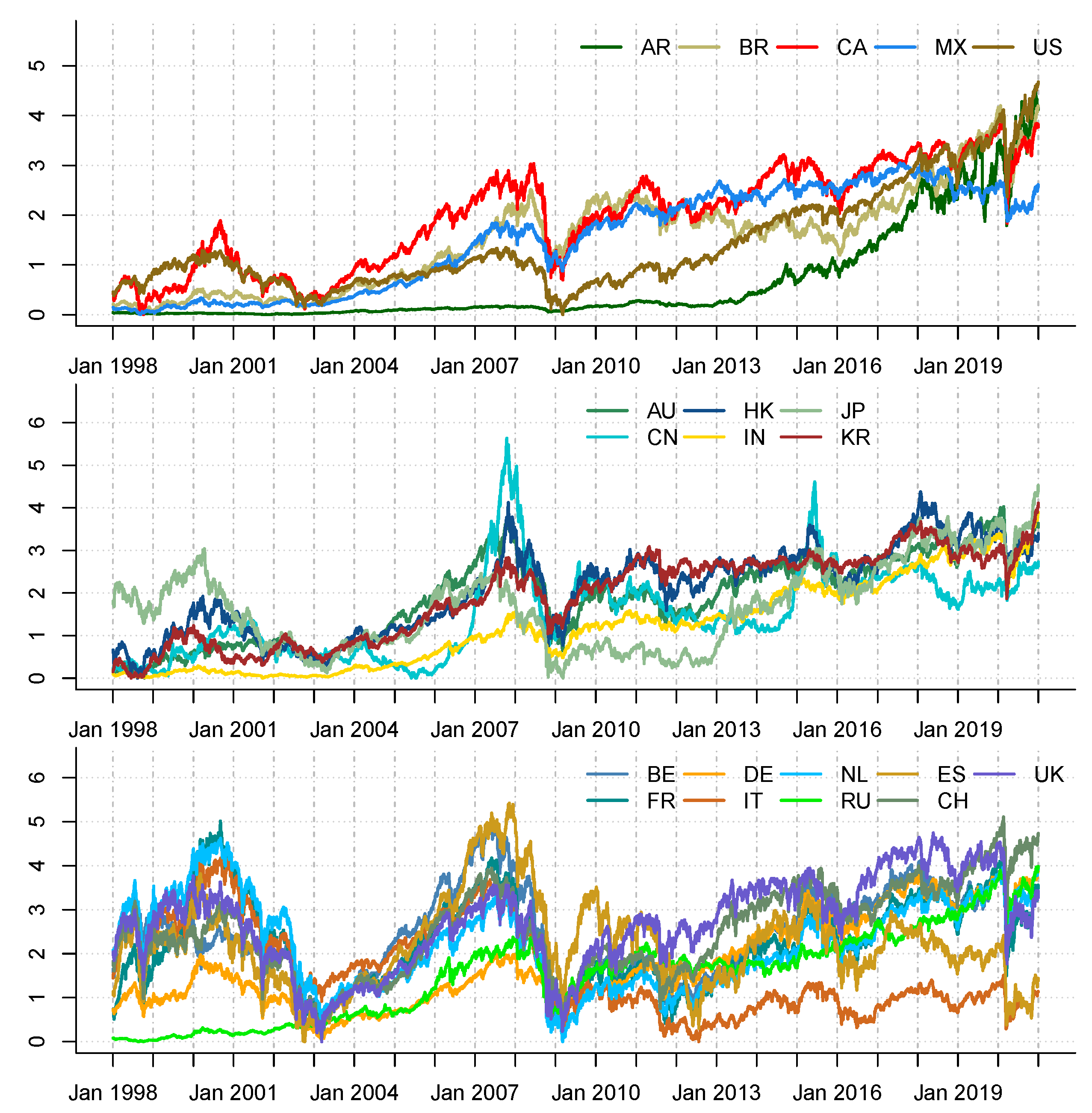
We report in Figure 1 the daily series of closing prices on a logarithmic scale. We scaled the prices to a zero mean and unit variance and added the absolute minimum value of each series to avoid negative outcomes. This standardises the scale of measurement for the different series.
The figure shows that over the past two decades, global financial markets have experienced several catastrophic events within and across different markets. Among these events are: (1) the dotcom “tech”-induced crisis of 2000–2003, which was fuelled by the adoption of the Internet in the late 1990s, triggering inflated stock prices that gradually went downhill and disrupted global market operations; (2) the global financial crisis of 2007–2009, which was triggered by the massive defaults of sub-prime borrowers in the U.S. mortgage market; (3) the European sovereign debt crisis of 2010–2013, which emanated from the inability of a cluster of EU member states to repay or refinance their sovereign debt and bailout heavily leveraged financial institutions without recourse to third-party assistance; (4) the distress to the world economy and global financial markets caused by the novel coronavirus pandemic in 2020.
We computed daily log returns as the log differences of successive daily closing prices. We also computed the daily expected shortfalls at the -quantile following (2) via a 22 d horizon rolling estimation of daily returns. Table 2 reports a set of summary statistics for the daily returns and daily change in expected shortfalls over the sample period.
From the summary statistics, almost all returns and daily change in the ES have a near-zero mean. The returns have a relatively high standard deviation, while the change in the ES recorded a relatively low standard deviation. The skewness of the returns indicates that all the indices have fairly symmetric distributions with mostly small, but consistent positive gains and, occasionally, large negative returns. The kurtosis of the returns and daily change in the ES indicates leptokurtic behaviours.
4. Empirical Findings
We studied the dynamics of the downside interconnectedness among the major stock markets via a yearly rolling window of 52 weeks. This is to capture year-on-year dependence among the markets. We set the increments between successive rolling windows to one week. The first window covers March 1998–March 1999 and the last from January 2019–December 2020. In total, we have 1140 windows.
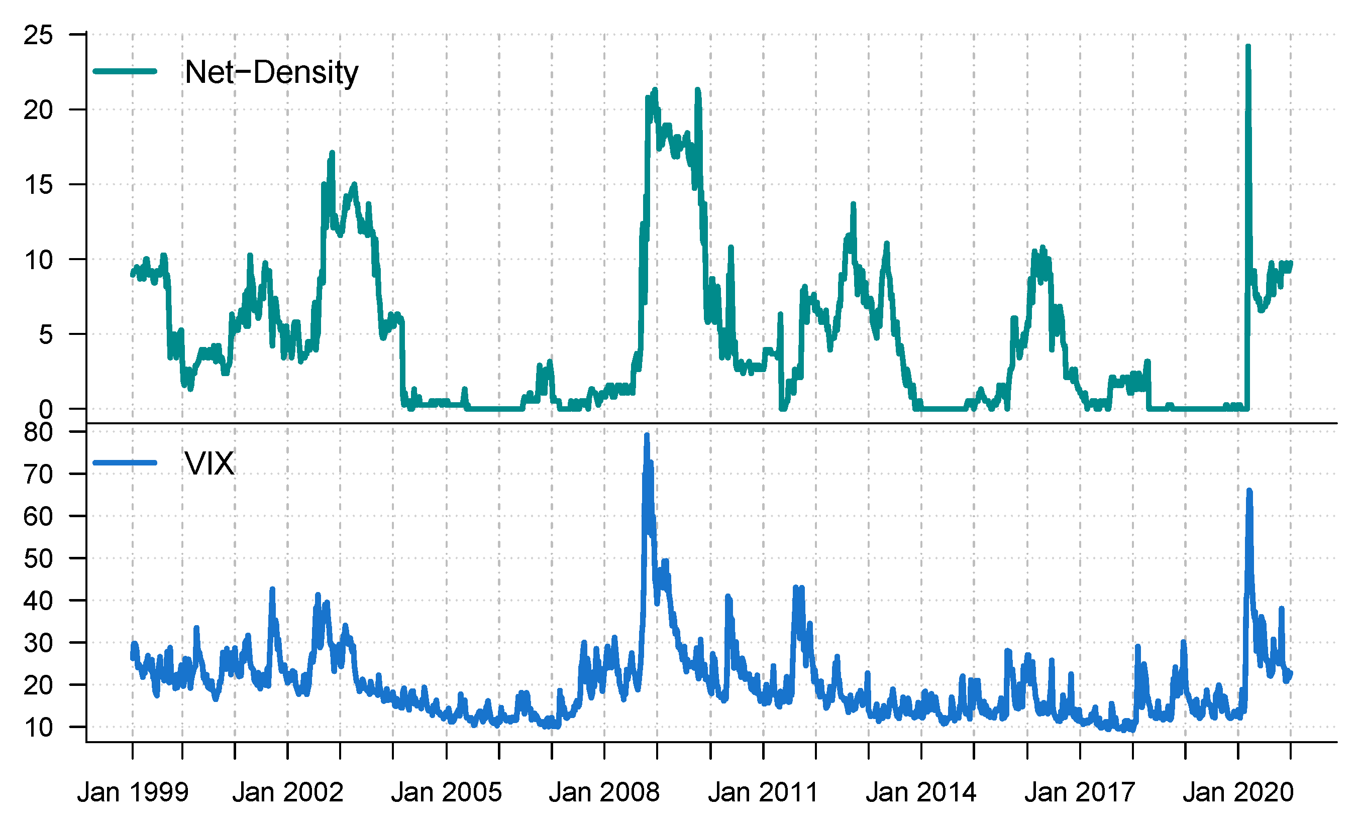
We characterised through numerical summaries the dynamic interconnectedness among the major stock markets by monitoring the network density against the VIX index—a measure that reflects the market’s expectation on the monthly volatility based on the S&P 500 index. The network density is given by the number of links in the estimated network divided by the total number of possible links.
Figure 2 shows the time series of the network density against the VIX. The figure shows a strong positive relationship between Net-Density and the VIX. Both indices indicate spikes during the tech-bubble crisis (2000–2003), the global financial crisis (GFC, 2007–2009), the Eurozone crisis (2010–2013), the oil crisis (2015–2016), and the corona crash (2020). The spikes in both indices at the onset of crisis periods indicate elevated levels of unusualness in the equity markets, a rise in financial market risk, and downside risk interconnectedness among stock markets. The historical highest Net-Density recorded in 2020 shows that the COVID-19-induced crisis was much greater than any market crisis in the last 20 years.
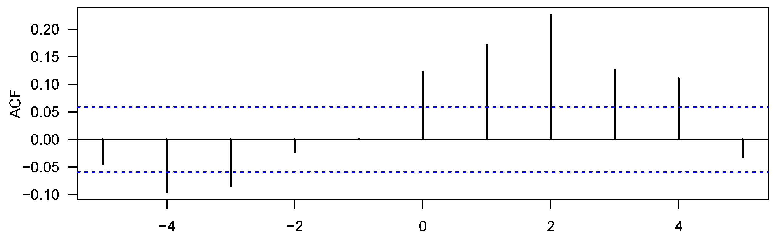
In the interest of analysing the relationship between downside risk interconnectedness and global market risk, we studied the lead–lag relationship between the Net-Density and VIX. We stationarised each series via first differencing. Figure 3 presents the results of the cross-correlation of the first difference of Net-Density and VIX.
The figure shows that the most significant cross-correlation between the Net-Density and the VIX occurred at lag zero. We also found evidence that the Net-Density preceded the VIX by two lags. This suggests that higher levels of downside risk interconnectedness preceded higher levels of financial market risk. Thus, the above findings show that the relationship between the network density of stock market downside risk interconnections and financial market risk is not a mere coincidence, but rather evidence of contagion. That is, periods of dense stock market downside risk interconnectedness increases global market risk. This is in line with the findings of [1,22], among others, for which dense interconnectedness does amplify financial market risk.
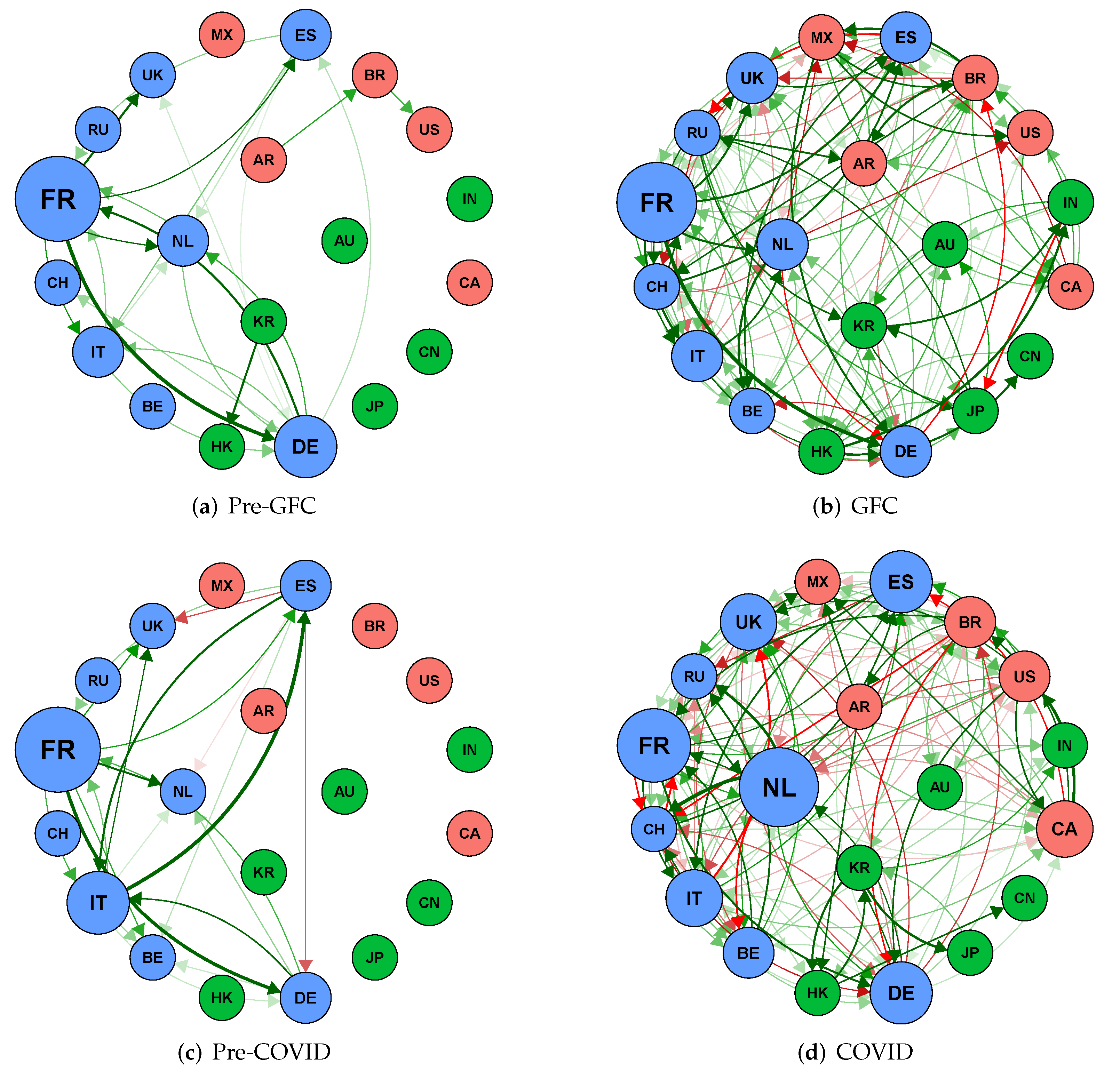
We present in Figure 4 the network topology of the interconnectedness divided into four sub-periods: pre-global financial crisis (pre-GFC: 29 January 1999–12 September 2008); the global financial crisis (GFC: 15 September 2008–25 December 2009); pre-COVID-19 (pre-COVID: 1 January 2010–14 February 2020); the COVID-19 outbreak (COVID: 21 February 2020–31 December 2020).
We compared the sub-period networks in terms of average degree, density, clustering coefficient, and average path length (see Table 3). We noticed that two sub-periods recorded tranquil conditions (i.e., 3 January 2000–12 September 2008 and 7 July 2009–20 February 2020), while the other two (15 September 2008–6 July 2009, and 21 February 2020–30 October 2020) experienced stressful conditions. The tranquil periods were characterised by a relatively low average degree of interconnectedness, a lower density and clustering index, and a relatively high average path length. This suggests a lower degree of equity market integration before and after the global financial crisis. It also shows that in the event of a shock to a major market or a group of major markets, these shocks will take a much longer time to propagate to other markets to cause a systemic breakdown.
Global Financial Crisis vs. COVID-19 Outbreak
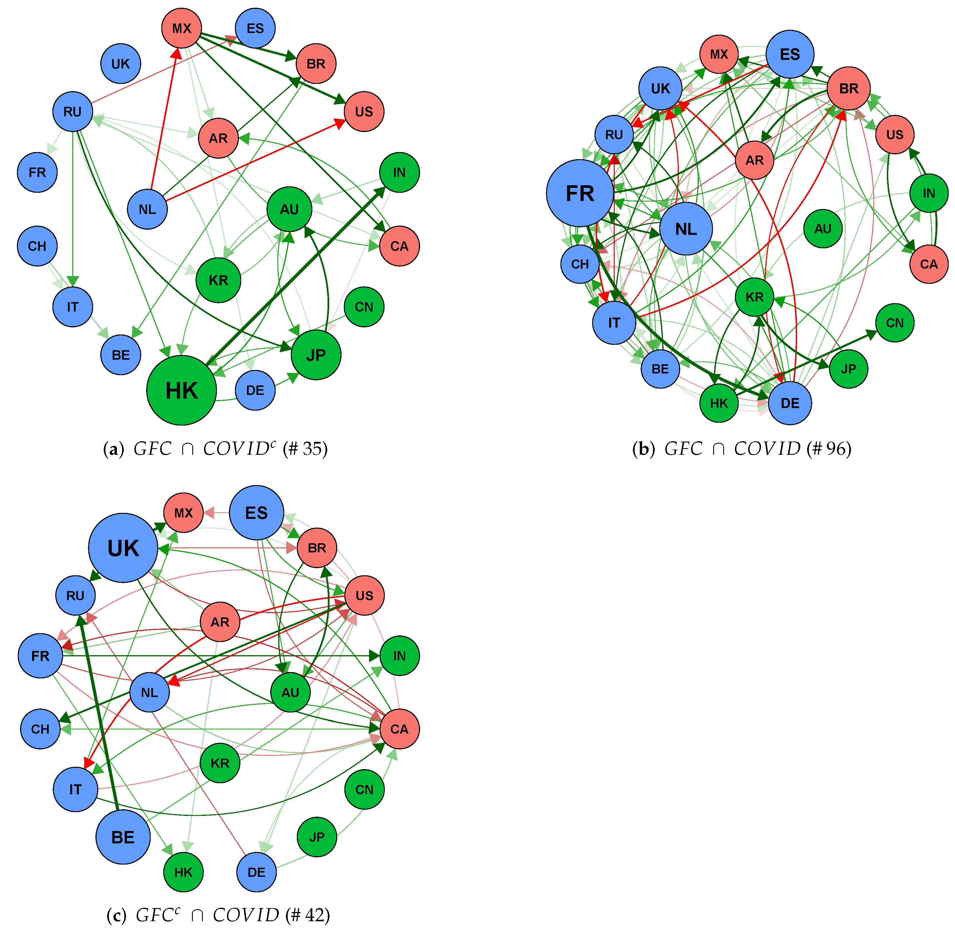
We compared the interconnectedness during the GFC and COVID-19 outbreak. To achieve this, we extracted the intersection and differences between the networks. Figure 5 presents the similarity and difference between the structure of interconnectedness during the GFC and COVID-19 sub-periods. Figure 5a depicts the network links during the GFC, but not in the COVID-19 period. Figure 5b displays the network links common to both periods, and Figure 5c shows only links in the COVID-19 period, but not present during the GFC.
Overall, we found 96 common connections between both networks. The GFC recorded 35 extra links that were not present in the COVID-19 network, and the latter also reported 42 new connections that were not in existence during the financial crisis.
We compared the most critical (or central) market to during what appears to be the two most-severe equity market crises over the last two decades. Table 4 reports the summary of the top five most-central markets in the downside risk propagation according to hub and authority scores over the two crisis sub-periods. The table shows that the top three transmitters of spillover propagation during the GFC were Germany, Italy, and The Netherlands, while the top three receivers were France, The Netherlands, and the U.K. During the COVID-19 outbreak, the most central markets for transmitting shocks were Switzerland, Russia, and Spain, while The Netherlands, France, and Spain ranked high at the receiving end of the downside risk. Thus, not only has the structure of the downside risk interconnectedness changed over the two crises, but the most central markets for spillover propagation have also changed in recent times.
5. Conclusions
We studied the sensitivity of stock returns to the tail risk of major equity market indices via the extreme downside hedge (EDH) model. The EDH model relies on the argument that in turbulent times, some assets/markets usually perform badly while others have mild reactions. Any asset that acts as a hedge to the tail risk of other assets/market indices is often high in demand and usually commands a price premium. The EDH was estimated by regressing asset returns on the tail risk of other assets/markets. We analysed the EDH relationship among the major equity indices via a Bayesian graph structural learning method. The empirical application examined whether downside risk connections among the major stock markets are merely anecdotal or provide the signal of contagion and the nature of sensitivity among major equity markets during the global financial crisis and the coronavirus pandemic.
The result showed strong evidence of tail risk interconnectedness among stock markets both in the tranquil period and during the crisis and post-crisis periods. We showed that during crisis periods (when markets are more vulnerable), the degree of interconnectedness is particularly stronger and more persistent, which implies losses for investors already with long stock exposures. We also found that the level of downside risk spillovers induced by COVID-19 recorded the highest network density, suggesting stronger evidence of contagion in the recent coronavirus pandemic than during the global financial crisis. The evidence showed that even though the most central equity markets for downside risk propagation changed over the two crises periods, the majority of the top five transmitters and recipients were EU-centred markets.
Funding
This research received no external funding.
Institutional Review Board Statement
Not applicable.
Informed Consent Statement
Not applicable.
Data Availability Statement
The data and the material used in the paper is publicly available on Yahoo Finance, but can also obtained from the authors upon request.
Acknowledgments
We would like to thank the editor and referees for their comments on an earlier version of this paper.
Conflicts of Interest
The authors declare no conflict of interest.
References
- Billio, M.; Getmansky, M.; Lo, A.W.; Pelizzon, L. Econometric Measures of Connectedness and Systemic Risk in the Finance and Insurance Sectors. J. Financ. Econ. 2012, 104, 535–559. [Google Scholar] [CrossRef]
- Diebold, F.; Yilmaz, K. On the Network Topology of Variance Decompositions: Measuring the Connectedness of Financial Firms. J. Econom. 2014, 182, 119–134. [Google Scholar] [CrossRef] [Green Version]
- Battiston, S.; Delli Gatti, D.; Gallegati, M.; Greenwald, B.; Stiglitz, J.E. Liaisons Dangereuses: Increasing Connectivity, Risk Sharing, and Systemic Risk. J. Econ. Dyn. Control 2012, 36, 1121–1141. [Google Scholar] [CrossRef] [Green Version]
- Billio, M.; Casarin, R.; Rossini, L. Bayesian Nonparametric Sparse VAR Models. J. Econom. 2019, 212, 97–115. [Google Scholar] [CrossRef] [Green Version]
- Harris, R.D.; Nguyen, L.H.; Stoja, E. Systematic Extreme Downside Risk. J. Int. Financ. Mark. Inst. Money 2019, 61, 128–142. [Google Scholar] [CrossRef]
- Ahelegbey, D.F.; Giudici, P.; Mojtahedi, F. Tail Risk Measurement In Crypto-Asset Markets. Int. Rev. Financ. Anal. 2021, 73, 101604. [Google Scholar] [CrossRef]
- Mojtahedi, F.; Mojaverian, S.M.; Ahelegbey, D.F.; Giudici, P. Tail Risk Transmission: A Study of the Iran Food Industry. Risks 2020, 8, 78. [Google Scholar] [CrossRef]
- Ahelegbey, D.F.; Billio, M.; Casarin, R. Bayesian Graphical Models for Structural Vector Autoregressive Processes. J. Appl. Econom. 2016, 31, 357–386. [Google Scholar] [CrossRef] [Green Version]
- Ahelegbey, D.F.; Billio, M.; Casarin, R. Sparse Graphical Vector Autoregression: A Bayesian Approach. Ann. Econ. Stat. 2016, 123/124, 333–361. [Google Scholar] [CrossRef]
- Paci, L.; Consonni, G. Structural Learning of Contemporaneous Dependencies in Graphical VAR Models. Comput. Stat. Data Anal. 2020, 144, 106880. [Google Scholar] [CrossRef]
- Gruber, L.F.; West, M. Bayesian Forecasting and Scalable Multivariate Volatility Analysis Using Simultaneous Graphical Dynamic Models. Econom. Stat. 2017, 3, 3–22. [Google Scholar]
- Chabi-Yo, F.; Ruenzi, S.; Weigert, F. Crash Sensitivity and the Cross Section of Expected Stock Returns. J. Financ. Quant. Anal. 2018, 53, 1059–1100. [Google Scholar] [CrossRef]
- Van Oordt, M.R.; Zhou, C. Systematic Tail Risk. J. Financ. Quant. Anal. 2016, 51, 685–705. [Google Scholar] [CrossRef]
- Almeida, C.; Ardison, K.; Garcia, R.; Vicente, J. Nonparametric Tail Risk, Stock Returns and the Macroeconomy. J. Financ. Econom. 2017, 15, 333–376. [Google Scholar]
- Hautsch, N.; Schaumburg, J.; Schienle, M. Financial Network Systemic Risk Contributions. Rev. Financ. 2015, 19, 685–738. [Google Scholar] [CrossRef] [Green Version]
- Härdle, W.K.; Wang, W.; Yu, L. TENET: Tail-Event driven NETwork risk. J. Econom. 2016, 192, 499–513. [Google Scholar] [CrossRef]
- Wang, G.J.; Yi, S.; Xie, C.; Stanley, H.E. Multilayer Information Spillover Networks: Measuring Interconnectedness of Financial Institutions. Quant. Financ. 2021, 21, 1–23. [Google Scholar] [CrossRef]
- Adrian, T.; Brunnermeier, M.K. CoVaR. Am. Econ. Rev. 2016, 106, 1705–1741. [Google Scholar] [CrossRef]
- Geiger, D.; Heckerman, D. Parameter Priors for Directed Acyclic Graphical Models and the Characterization of Several Probability Distributions. Ann. Stat. 2002, 30, 1412–1440. [Google Scholar] [CrossRef]
- Ahelegbey, D.F.; Giudici, P. NetVIX-A Network Volatility Index of Financial Markets. Phys. A Stat. Mech. Its Appl. 2022, 594, 127017. [Google Scholar] [CrossRef]
- Gelman, A.; Rubin, D.B. Inference from Iterative Simulation Using Multiple Sequences, (with discussion). Stat. Sci. 1992, 7, 457–511. [Google Scholar] [CrossRef]
- Blume, L.; Easley, D.; Kleinberg, J.; Kleinberg, R.; Tardos, É. Network Formation in the Presence of Contagious Risk. ACM Trans. Econ. Comput. 2013, 1, 6. [Google Scholar] [CrossRef] [Green Version]
Figure 1.
Time series of daily equity log prices from January 1998 to December 2021, by regional classification: Americas (top), Asia-Pacific (middle), and Europe (bottom).
Figure 1.
Time series of daily equity log prices from January 1998 to December 2021, by regional classification: Americas (top), Asia-Pacific (middle), and Europe (bottom).

Figure 2.
Network density and VIX index.

Figure 3.
Correlation of with .

Figure 4.
Sub-period downside risk transmission network among stock markets. Red nodes represent the markets of the Americas, blue for Europe, and green for Asia-Pacific. The size of the nodes is out-degree weighted. Red links denote negative sensitivity and green for positive reactions.
Figure 4.
Sub-period downside risk transmission network among stock markets. Red nodes represent the markets of the Americas, blue for Europe, and green for Asia-Pacific. The size of the nodes is out-degree weighted. Red links denote negative sensitivity and green for positive reactions.

Figure 5.
Comparing the global financial crisis (GFC) and COVID-19 outbreak network. Red nodes represent the markets of the Americas, blue for Europe, and green for Asia-Pacific. The size of the nodes is out-degree weighted. Red links denote negative effects and green for positive interactions. The number in parenthesis signifies the total links in each network. Note: —complement of A.


Table 1.
Detailed description of the stock market indices of countries classified according to regions.
Table 1.
Detailed description of the stock market indices of countries classified according to regions.
| Region | No. | Country | Code | Description | Index |
|---|---|---|---|---|---|
| 1 | Argentina | AR | Argentina MERVAL | MERVAL | |
| 2 | Brazil | BR | Brazil Bovespa | IBOV | |
| Americas | 3 | Canada | CA | Canada TSX Comp. | SPTSX |
| 4 | Mexico | MX | Mexico IPC | MEXBOL | |
| 5 | United States | US | United States S&P 500 | SPX | |
| 6 | Australia | AU | Australia ASX 200 | AS51 | |
| 7 | China | CN | China SSE Comp. | SHCOMP | |
| Asia-Pacific | 8 | Hong Kong | HK | Hong Kong Hang Seng | HSI |
| 9 | India | IN | India BSE Sensex | SENSEX | |
| 10 | Japan | JP | Japan Nikkei 225 | NKY | |
| 11 | Korea | KR | South Korean KOSPI | KOSPI | |
| 12 | Belgium | BE | Belgium BEL 20 | BEL20 | |
| 13 | France | FR | France CAC 40 | CAC | |
| 14 | Germany | DE | Germany DAX 30 | DAX | |
| 15 | Italy | IT | Italy FTSE MIB | FTSEMIB | |
| Europe | 16 | The Netherlands | NL | The Netherlands AEX | AEX |
| 17 | Russia | RU | Russia MOEX | IMOEX | |
| 18 | Spain | ES | Spain IBEX 35 | IBEX | |
| 19 | Switzerland | CH | Switzerland SMI | SMI | |
| 20 | United Kingdom | UK | U.K. FTSE 100 | UKX |
Table 2.
Statistics of daily returns and change in the ES for stock markets (March 1998–December 2020).
Table 2.
Statistics of daily returns and change in the ES for stock markets (March 1998–December 2020).
| Daily Returns | Daily Log ES | |||||||
|---|---|---|---|---|---|---|---|---|
| Code | Mean | SD | Skew | Kurt | Mean | SD | Skew | Kurt |
| AR | 0.0775 | 2.2776 | −1.7342 | 35.0728 | −0.0154 | 63.4156 | −5.9109 | 820.8923 |
| BR | 0.0373 | 1.9175 | 0.2348 | 15.7679 | −0.0249 | 64.1751 | −21.0317 | 1841.0830 |
| CA | 0.0182 | 1.0978 | −0.9401 | 16.8512 | −0.0298 | 21.5994 | 1.8971 | 254.6383 |
| MX | 0.0384 | 1.3268 | 0.1088 | 6.4837 | −0.0678 | 22.4015 | 0.3937 | 74.0335 |
| US | 0.0246 | 1.2155 | −0.3997 | 10.9808 | −0.0285 | 20.8834 | −1.4264 | 133.3279 |
| AU | 0.0168 | 0.9926 | −0.6961 | 8.5250 | −0.0150 | 16.3888 | 1.4337 | 138.1182 |
| CN | 0.0171 | 1.4756 | −0.3506 | 5.6949 | −0.0557 | 38.1862 | −2.6821 | 189.0206 |
| HK | 0.0136 | 1.4693 | −0.0185 | 7.1981 | −0.0925 | 25.9796 | −0.8570 | 142.6127 |
| IN | 0.0463 | 1.4532 | −0.2802 | 8.8733 | −0.0176 | 43.0280 | −5.6080 | 812.9438 |
| JP | 0.0087 | 1.4343 | −0.3390 | 6.4696 | −0.0055 | 31.0559 | −3.3666 | 219.1089 |
| KR | 0.0284 | 1.5794 | −0.2769 | 6.4429 | −0.0696 | 29.0712 | −0.1575 | 269.9062 |
| BE | 0.0075 | 1.2404 | −0.4001 | 9.5224 | −0.0072 | 22.4958 | 1.6991 | 239.2680 |
| FR | 0.0128 | 1.4137 | −0.2117 | 6.2409 | −0.0191 | 26.2744 | −3.4356 | 280.8779 |
| DE | 0.0202 | 1.4631 | −0.1968 | 5.6709 | −0.0334 | 23.6652 | 0.0171 | 143.6197 |
| IT | −0.0008 | 1.5230 | −0.5382 | 8.5133 | −0.0058 | 31.5024 | −5.9900 | 457.8811 |
| NL | 0.0096 | 1.3822 | −0.2423 | 7.0535 | −0.0097 | 21.5194 | 0.1786 | 106.0908 |
| RU | 0.0648 | 2.2908 | 0.2812 | 19.9011 | −0.1418 | 45.9988 | −0.4843 | 141.6174 |
| ES | 0.0014 | 1.4612 | −0.3061 | 7.6552 | −0.0023 | 33.7401 | 0.4265 | 293.9172 |
| CH | 0.0095 | 1.1575 | −0.2895 | 7.5521 | −0.0252 | 21.6889 | 3.1533 | 219.5005 |
| UK | 0.0044 | 1.1715 | −0.3089 | 7.5820 | −0.0173 | 18.6884 | −0.1894 | 96.3411 |
Table 3.
The network statistics for sub-period interconnectedness graphs.
| No. | Sub-Period | Average Degree | Density | Clustering Coefficient | Average Path Length |
|---|---|---|---|---|---|
| 1 | Pre-GFC | 1.150 | 6.053 | 0.733 | 1.324 |
| 2 | GFC | 6.550 | 34.474 | 0.754 | 2.211 |
| 3 | Pre-COVID-19 | 1.100 | 5.789 | 0.814 | 1.083 |
| 4 | COVID-19 | 6.900 | 36.316 | 0.787 | 1.734 |
Table 4.
Top 5 centrality ranking during the global financial crisis and COVID-19 pandemic.
| Rank | GFC | COVID | ||||||
|---|---|---|---|---|---|---|---|---|
| Hub | Auth | Hub | Auth | |||||
| 1 | DE | 0.471 | FR | 0.884 | CH | 0.411 | NL | 0.560 |
| 2 | IT | 0.378 | NL | 0.252 | RU | 0.335 | FR | 0.454 |
| 3 | NL | 0.373 | UK | 0.211 | ES | 0.330 | ES | 0.329 |
| 4 | UK | 0.367 | IT | 0.158 | DE | 0.308 | DE | 0.314 |
| 5 | ES | 0.354 | ES | 0.141 | BR | 0.294 | CA | 0.269 |
Publisher’s Note: MDPI stays neutral with regard to jurisdictional claims in published maps and institutional affiliations. |
© 2022 by the author. Licensee MDPI, Basel, Switzerland. This article is an open access article distributed under the terms and conditions of the Creative Commons Attribution (CC BY) license (https://creativecommons.org/licenses/by/4.0/).
Share and Cite
MDPI and ACS Style
Ahelegbey, D.F. Statistical Modelling of Downside Risk Spillovers. FinTech 2022, 1, 125-134. https://doi.org/10.3390/fintech1020009
AMA Style
Ahelegbey DF. Statistical Modelling of Downside Risk Spillovers. FinTech. 2022; 1(2):125-134. https://doi.org/10.3390/fintech1020009
Chicago/Turabian StyleAhelegbey, Daniel Felix. 2022. "Statistical Modelling of Downside Risk Spillovers" FinTech 1, no. 2: 125-134. https://doi.org/10.3390/fintech1020009