
Shapley Feature Selection


Department of Economics and Management, Neosurance and University of Pavia, 27100 Pavia, PV, Italy
*
Author to whom correspondence should be addressed.
FinTech 2022, 1(1), 72-80; https://doi.org/10.3390/fintech1010006
Submission received: 11 January 2022
/
Revised: 14 February 2022
/
Accepted: 21 February 2022
/
Published: 25 February 2022
(This article belongs to the Special Issue Fintech and Sustainable Finance)
Abstract
:Feature selection is a popular topic. The main approaches to deal with it fall into the three main categories of filters, wrappers and embedded methods. Advancement in algorithms, though proving fruitful, may be not enough. We propose to integrate an explainable AI approach, based on Shapley values, to provide more accurate information for feature selection. We test our proposal in a real setting, which concerns the prediction of the probability of default of Small and Medium Enterprises. Our results show that the integrated approach may indeed prove fruitful to some feature selection methods, in particular more parsimonious ones like LASSO. In general the combination of approaches seems to provide useful information which feature selection algorithm can improve their performance with.
1. Introduction
Feature selection is an area of research of great importance in machine learning. At the end of the last century, when a special issue on relevance including several papers on variable and feature selection was published [1], very few domains used more than 40 features in their models ([2]). The situation has changed drastically over the years, due to the increased capability to collect more data and to process multidimensional data. The problem with these developments is that, with so many dimensions, we also introduce many irrelevant or redundant features and often we have comparably few training examples. This hinders the ability of the model to generalize to predictions [3] and, also, it increases its complexity, therefore its cost. Furthermore, there are many potential advantages in performing an effective feature selection: easier data visualization and explanation, lower requirements for measuring and storing data, lower training and utilization time, more easily performed sensitivity analysis. Moreover, feature selection helps to reduce the risk of incurring in overfitting due to the curse of dimensionality, and this increases performance and robustness.
In the available literature, there are a variety of methods which perform feature selection but there is no single method which is appropriate for all types of problems. The main directions that have been taken to tackle the issue originally divide into wrappers, filters and embedded methods (see Stanczyk, 2015 [4]), up to more innovative approaches like Swarm Intelligence (see for instance Brezočnik et al. [5]) and similarity classifier used in combination with a new fuzzy entropy measure in signal processing (see Tran, Elsisi, Liu [6]). Wrappers utilize the chosen machine learning model to score many different subsets of variables according to their predictive power, in an often greedy and computationally intensive approach; filters select the variables of interest as a pre processing step, independently of the chosen predictor; embedded methods are peculiar to certain kinds of models which perform variable selection in the process of training. Each of these approaches has its strengths and weaknesses, which make them suitable or not for a specific problem. Many algorithms have been developed, especially in the wrapper field, to improve selection robustness and relevance, but increase in the complexity of algorithms limits the effectiveness of the proposal. What would be interesting, instead, is looking for an integrated approach, and see if a contamination of methods can actually bring some benefit and improvements to feature selection.
Our contribution with this paper is to try and improve feature selection by combining the Shapley value framework (SHAP for brevity) with different feature selection approaches. We do this in order to take advantage of its many desirable properties (Lundberg et al., 2017 [7]): local accuracy, missingness and consistency, in their role of variable importance determination, adding to the literature that employs Shapley values a post-processing phase (see for instance Bussman et al., 2020 [8] and Gramegna and Giudici, 2020 [9]). We show that SHAP can indeed extract futher information from the nexus data-predictive model, and that such information can be useful in selecting relevant features.
Our proposal will be tested on a real dataset, provided by the fintech company MonAI, which among other things provides eXplainable credit scores to SMEs and professionals, using both traditional and alternative data. The aim of the application is to be able to select an adequate number of features, so to have a model which is both well explainable and performing, in the setting of probability of default prediction for the considered companies.
The remainder of the paper is organized as follows. The “Data and methods” section provides an overview of the data employed and of the tested methods. The “Results” section presents our results. Finally, conclusions and future research directions are indicated in “Conclusion and future work” section.
2. Methods
2.1. Data
The data we use to test our methodology is quite traditional, being balance sheet data from the last six years belonging to italian SMEs. We can find all the classical balance sheet entries, together with some composite indexes (e.g., leverage, Return on Sales—these will be masked with the letter V and numbers from 1 to 30). In a pre processing step, we have eliminated some linear combinations inherently present in the data (as done in filter methods). As a result, we have 49 features.
We then employed statistical tools to deal with strongly unbalanced classes (e.g., Lin et al. (2017) [10]), since defaults were slightly more than 1%, and to remove time-specific factors. More specifically, we employed data encompassing five years (2015 to 2019), comprising more than two millions of SME observations, keeping all the defaulted cases and randomly sampling a group of non-defaulted firms equal to about 10000 for each year. With the remaining observations we build 5000 clusters per year and employ the cluster medoids as input observations (the same way we did it in Gramegna and Giudici, 2021 [11]). This brought down class imbalance from about 100:1 to 5:1, allowing the model to better frame risk patterns and give more amplitude to probability estimation. The above procedure has led us to a training dataset of about 139,000 observations, with 27,200 defaults; the entire year 2020 was left out from pre processing in order to have a clean, validation set to test our proposed methods. We performed stratified sampling for training and testing set to maintain the balance for the positive and negative class of the Y variable.
2.2. Models
2.2.1. LightGBM
To learn the default pattern from the data and be able to provide a probabilistic estimate for each observation, we use an improved implementation of XGBoost (Chen and Guestrin, 2016 [12]), called LightGBM. This is a gradient boosted tree model very similar to XGBoost, which features the suggestions of Ke G., Finley T., et al. [13] which strongly increase efficiency and scalability, greatly improving the standard gradient boosting tree model (by about 20 times). LightGBM, on the top of featuring a light and fast implementation, differs from other gradient boosted tree models in that while other algorithms grow trees horizontally, LightGBM algorithm grows them vertically, meaning it grows leaf-wise while other algorithms of the family grow level-wise. LightGBM chooses the leaf with the largest loss to grow the next tree: in doing so, it can lower loss more than a level wise algorithm, since it originates less redundant leaves. It also employs binarization of continuous variables, which reduces computation time a lot because there is no need to evaluate the entire range of the continuous variables and to run dispendious sorting algorithms. This way of working also makes it less suitable for small datasets, where it can easily overfit due to its sensitivity. All the above elements make lightGBM suitable to us, as we need to run the model multiple times, and on a rather big dataset.
2.2.2. SHAP
The SHAP framework has been proposed by Lundberg, 2017 [7] adapting a concept from game theory (Shapley (1952) [14]), and has many attractive properties. With SHAP, the variability of the predictions is divided among the available features; in this way, the contribution of each explanatory variable to each point prediction can be assessed regardless of the underlying model (Joseph (2019) [15]). From a computational perspective, the SHAP framework returns Shapley values which express model predictions as linear combinations of binary variables that describe whether each covariate is present in the model or not.
More formally, the SHAP algorithm approximates each prediction with , a linear function of the binary variables and of the quantities , defined as follows:
where M is the number of explanatory variables.
Lundberg, (2018) [16] has shown that the only additive method that satisfies the properties of local accuracy, missingness and consistency is obtained attributing to each variable an effect (the Shapley value), defined by:
where f is the model, x are the available variables, and are the selected variables. The quantity expresses, for each single prediction, the deviation of Shapley values from their mean: the contribution of the i-th variable.
We will use SHAP values as transformed data input to feed to feature selection methods and see how it compares with feature selections made on the original data values.
2.3. Feature Selection
2.3.1. Stepwise Feature Selection
It is a wrapper algorithm well-known in the statistical and data science communities. It performs a classical greedy approach which tests the predictive performance of different subsets of variables in a stepwise fashion. This because optimisation methods based on best subset selection quickly become intractable and prone to overfitting when p is large. Unlike best subset selection, which involves fitting models, forward stepwise selection involves fitting one null model, along with models in the kth iteration, for k = 0,…, . This amounts to a total of models. This is a substantial difference: when , best subset selection requires fitting 1,048,576 models, whereas forward stepwise selection requires fitting only 211 models.
Here we use an adaptation of the stepwise approach which evaluates the feature covariates in terms of predictive performance and is allowed to go in both directions when sequentially adding the variables. Basically, after adding each new variable, the method may also remove any variables that no longer provide an improvement to the model fit. Such an approach attempts to more closely mimic best subset selection while retaining the computational advantages of forward and backward stepwise selection. The details of the algorithm are described in Introduction to Statistical Learning, by James, Witten, Hastie and Tibshirani [17]. This feature selection method, being a wrapper, has the benefit of being “supervised”, in the sense that we evaluate the performance of the variables directly on the output, so it is generally quite effective in identifying the most important variables. The cons are of course the computation cost which, though not as high as for best subset selection, is still something to consider; another downside of the method is that, differently from best subset selection, you are not guaranteed to select the best possible variables in term of predictive power, since this depends on the starting point and gradual inclusion of the variables, though parallel progressive exclusion of newly redundant variables does help in minimizing the problem.
2.3.2. LASSO
The Lasso method, short for Least Absolute Shrinkage and Selection Operator, is a linear model proposed by Tibshirani in 1995. It minimizes the residual sum of squares subject to the sum of the absolute value of the coefficients being less than a constant; because of the nature of this constraint it tends to produce some coefficients that are set exactly to 0 and therefore gives interpretable models. More formally, lasso regression adds “absolute value of magnitude” (L1 penalty) of coefficient as penalty term to the loss function, as we can see at the end of the below equation
On the contrary, ridge regression, as a shrinkage method, adds “squared magnitude” of coefficients as a penalty term to the loss function (L2 penalty)
Tibshirani’s simulation studies suggest that the lasso enjoys some of the favourable properties of both ridge regression and subset selection [18], making it an important example of embedded feature selection, which we will use in our application. LASSO has the advantage of having a low computation cost, since it is the cost of estimating regression parameters subject to penalty term; furthermore, it builds parsimonious models. On the other hand, it doesn’t necessarilty select the most informative features and sometimes the variables selected are just too few.
2.3.3. BORUTA
The last feature selection methods we will employ is of particular interest because, in the implementation we will use, it already uses SHAP values within its algorithm to evaluate the importance of features. Boruta is a wrapper built around the random forest algorithm [19], based on two main ideas. The first is to generate “shadow features” by perturbing the original features to create a randomized version of them. These shadow features are then added to the model as further covariates and the threshold for variable importance becomes the highest of these shadow features, according to the intuition that a feature is useful only if it is capable of doing better than the best randomized feature. The second idea is to iterate the outlined process n times and use the binomial distribution to evaluate the importance of the feature in a probabilistic manner; that is, if it passes the threshold or not, in n trials (see Kursa et al., 2010 [20]).
Using SHAP instead of classical metrics of feature importance, such as gain, split count and permutation, can be e a nice improvement because SHAP values have proprieties, as we have seen, that allow to assess variable importance in a more thorough and consistent way.
Thanks to the above processes, Boruta is a wrapper with a somewhat different flavour with respect to other wrapper feature selection algorithms. The idea of the shadow features, combined with SHAP importance as feature score, allows it to be very effective in selecting relevant variables. Nevertheless, it’s computation cost is high, since it is the cost of running the base model, estimating SHAP values and then iterate n times to perform the t-test. It also does not build parsimonious models, since it will select variables which deliver every bit of information. It is great if your goal is to eliminate noise.
3. Results
To compare the three proposed feature selection methods, we have applied them both to the regular dataset, with actual observations for each variable, and to a dataset made up of the SHAP values corresponding to each observation. The dimension of the data is the same in both cases.
We have then obtained the selected features under each of the three methods and for both versions of the dataset, then used a LightGBM model to assess the predictive power of the subsets.
Before comparing the performance of the considered feature selection models, we remark that the performance of the LightGBM model with all the available 49 features, as measured by the Area Under the Curve (AUC) calculated on the test set, is equal to AUC = 0.8706, with an F1 score of 0.5451. We highlight that we used the mean default probability as cutoff value to binarize the target variable for simplicity of comparison; there may be some other threshold that better maximise F1 score.
In the Table 1 we can see the Area Under the Curve (AUC) values for each of our proposed feature selection algorithms.
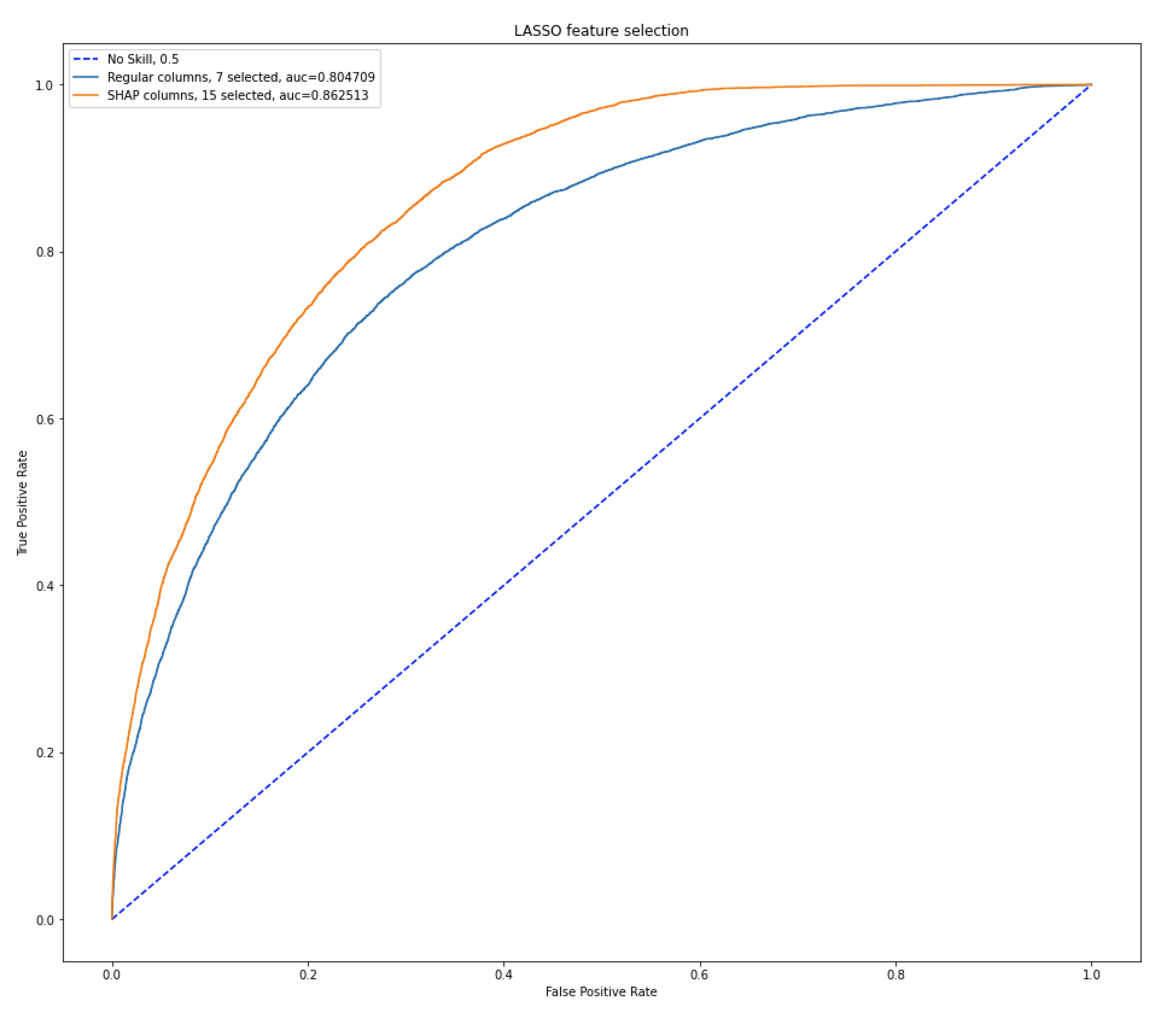
The above table empirically shows the well known trade off between explainability (better for models with fewer features) and predictive accuracy (better for models with more features). For instance, the model with only seven features selected is easier to explain but performs worse than the others. Indeed, LASSO applied to the original data is the model that leads to only seven features. This is due to the fact that it is the most parsimonious and that the marginal improvement in performance of adding a feature is lower than with other methods, as features that contribute the most are selected first.
The Lasso method applied to the SHAP dataset looks more appealing: it selects fifteen features, much less than the original 49, and with a performance that is almost as good as that obtained with the full dataset. In addition, we can take advantage of its computational speed, due to its belonging to the embedded family.
Figure 1 compares the ROC curves obtained with the two LASSO methods: that on the original data, and that based on Shapley values.
ROC curve comparison in Figure 1 reinforce the previous comment: the LASSO on the SHAP values performs better than that on the original data.
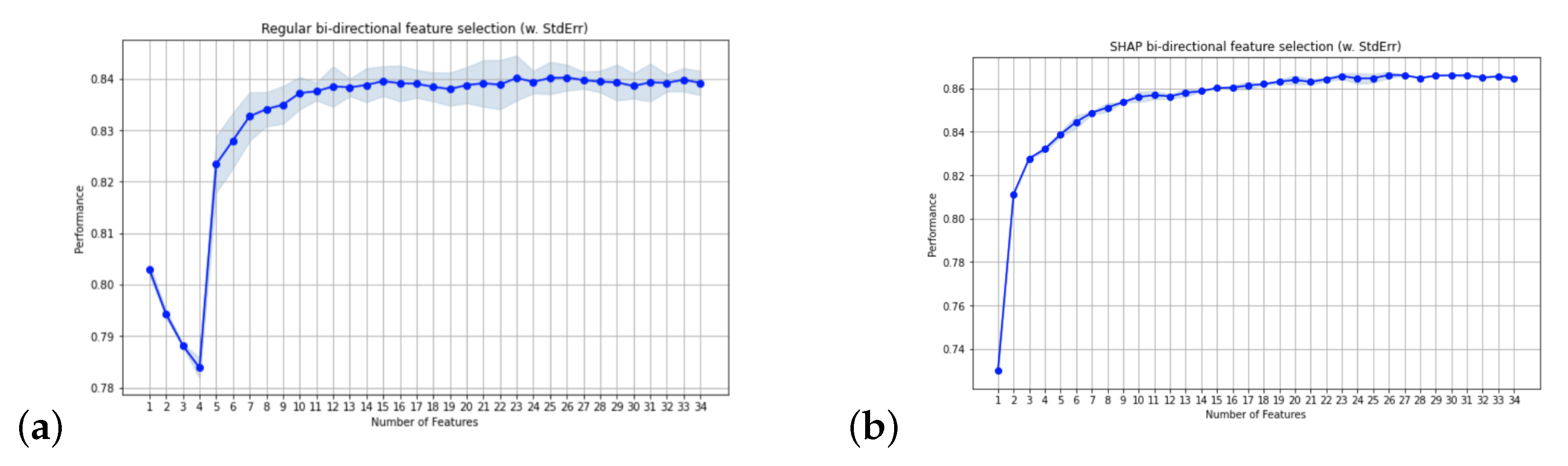
We now move to stepwise feature selection, which compares the performances of adding/deleting a variable feature, trying to reduce the search space. The previous table shows that the selected number of features is quite similar with both datasets, with number of variables selected from the SHAP data being slightly higher than those selected on the original data (33 against 27). The performances are also quite similar, as we expect dealing with this kind of data and with a relatively high number of selected variables.
Figure 2 compares the AUC performance of the stepwise method, for either datasets (original or SHAP), as the number of variables increase.
From Figure 2 we can see that the stepwise method on the SHAP data is quicker in achieving a high performance.
We now consider the third feature selection method, Boruta. From the previous table, the number of features selected is quite different for the two considered datasets (original and SHAP). In particular, the feature selection made on the SHAP dataset leads to a model which is almost the same as the full set. Precisely, it has four less variables (45 vs. 49) and, therefore, it manages to remove some noise; nevertheless, it performs very little selection. The same cannot be said for the selection made on the regular original set, where we see basically the same predictive performance as with all variables with just twenty six features. The apparent disadvantage of using SHAP values, which appears only for the Boruta method, can be explained by the fact that Boruta already uses SHAP and, therefore, using it twice is not of advantage since, as we said in the description of Boruta feature selection algorithm, this method is capable of picking up even the slightest bit of information from a variable, and the transformed SHAP dataset is made in a way that virtually every variable carry some more information with respect to base dataset.
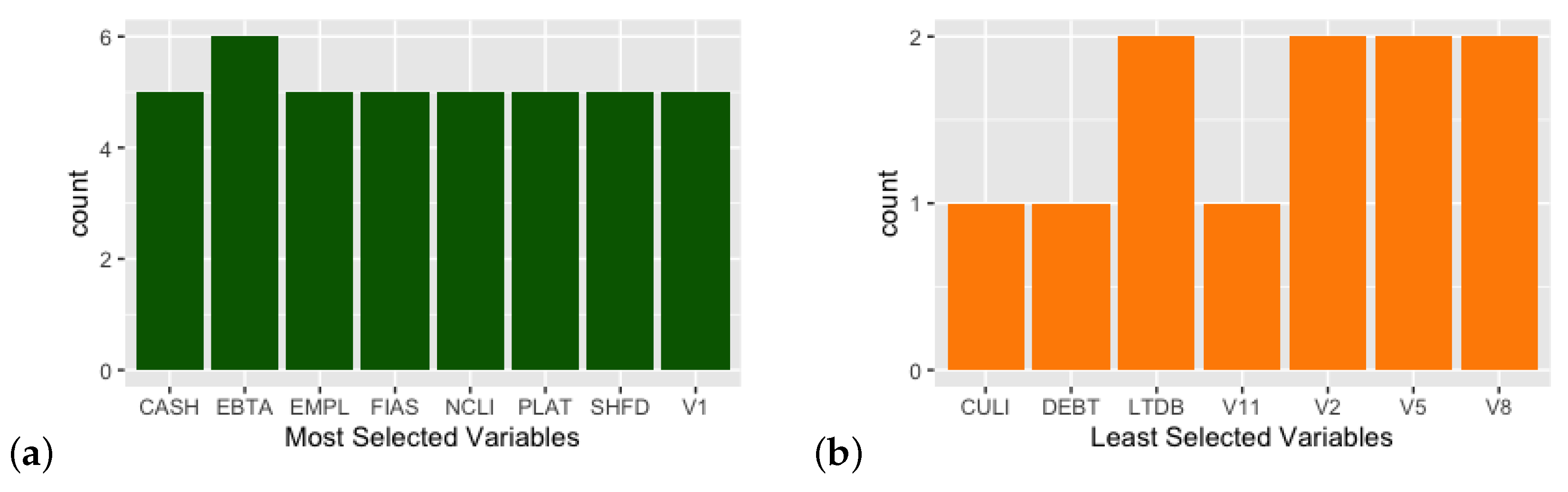
We also consider the variables which were effectively selected by different methods by making a comparison between the overall most selected variables and overall least selected ones in Figure 3. The methods were generally consistent in their selection, meaning that the more parsimonious methods chose variables that were also selected by more permissive algorithms, thus without overthrowing the underlying logic.
We find some expected variables among the most selected ones, such as CASH (availability of liquid resources), EBTA (EBIDTA) and PLAT (Profit and Loss After Taxes); we may have expected a more involved role for debt variables (DEBT, LTDB and CULI), but this could be explained by the fact that we plugged in many balance sheet variables, together with some indexes (V1 to V12 variables), and relevant information is probably provided by complementary measures and/or ratios. This makes sense since overall debt taken as stand-alone measure does not necessarily imply a bad situation; it only has meaning when compared to other entries such as turnover, current assets and so on.
We finally remark that so far we have been comparing models on the test set, which comes from the same data preprocessing we used for the training set. To fully assess the usefulness of SHAP as a contributor to feature selection methods, we should compare the performance of all feature selection models, against that of the full model, on new, unprocessed data. We present this comparison in the next Table 2, using the clean data from 2020.
4. Conclusions and Future Works
In the paper, we have suggested to apply feature selection methods on the data transformed into Shapley values. Our findings show that this does improve model performance and can also reduce computational costs.
The findings also show that the best trade-off between parsimony and predictive power is obtained with a LASSO feature selection method applied to the SHAP-transformed dataset.
Future works should continue to build and investigate the possibility of integrating Shapley values with statistical model selection, as recently seen in the literature of network models (Giudici et al., 2020 [21]), and on stochastic ordering (Giudici and Raffinetti, 2020 [22] and Giudici and Raffinetti 2021 [23]). It would be interesting to test the approach in different domains and within other feature selection algorithms, for instance in the medical domain (see Baysal et al., 2020 [24]) or in remote sensing (see Janowski et al., 2022 [25]).
Author Contributions
Both authors contribute equally to this research work. All authors have read and agreed to the published version of the manuscript.
Funding
This research received no external funding.
Institutional Review Board Statement
Not applicable.
Informed Consent Statement
Not applicable.
Data Availability Statement
Not applicable.
Conflicts of Interest
The authors declare no conflict of interest.
References
- Subramanian, D.; Greiner, R.; Pearl, J. Land Economics. Relevance 1997, 97, 1–2. [Google Scholar]
- Guyon, I.; Elisseeff, A. An Introduction to Variable and Feature Selection. J. Mach. Learn. Res. 2003, 3, 1157–1182. [Google Scholar]
- Chen, X.; Wasikowski, M. FAST: A Roc-Based Feature Selection Metric for Small Samples and Imbalanced Data Classification Problems. In Proceedings of the 14th ACM SIGKDD International Conference on Knowledge Discovery and Data Mining, Las Vegas, NV, USA, 24–27 August 2008; pp. 124–132. [Google Scholar]
- Stanczyk, U. Feature Evaluation by Filter, Wrapper, and Embedded Approaches. Stud. Comput. Intell. 2015, 584, 29–44. [Google Scholar]
- Brezočnik, L.; Fister, I.; Podgorelec, V. Swarm Intelligence Algorithms for Feature Selection: A Review. Appl. Sci. 2018, 8, 1521. [Google Scholar] [CrossRef] [Green Version]
- Tran, M.Q.; Elsisi, M.; Liu, M.K. Effective feature selection with fuzzy entropy and similarity classifier for chatter vibration diagnosis. Measurement 2021, 184, 109962. [Google Scholar] [CrossRef]
- Lundberg, S.M.; Lee, S.I. A Unified Approach to Interpreting Model Predictions. arXiv 2017, arXiv:1705.07874. [Google Scholar]
- Bussmann, N.; Giudici, P.; Marinelli, D.; Papenbrock, J. Explainable AI in Fintech Risk Management. Front. Artif. Intell. 2020, 3, 26. [Google Scholar] [CrossRef] [PubMed]
- Gramegna, A.; Giudici, P. Why to Buy Insurance? An Explainable Artificial Intelligence Approach. Risks 2020, 8, 137. [Google Scholar] [CrossRef]
- Lin, W.C.; Tsai, C.F.; Hu, Y.H.; Jhang, J.S. Clustering-based undersampling in class-imbalanced data. Inf. Sci. 2017, 409-410, 17–26. [Google Scholar] [CrossRef]
- Gramegna, A.; Giudici, P. SHAP and LIME: An Evaluation of Discriminative Power in Credit Risk. Front. Artif. Intell. 2021, 4, 140. [Google Scholar] [CrossRef] [PubMed]
- Chen, T.; Guestrin, C. XGBoost: A Scalable Tree Boosting System. In Proceedings of the 22nd ACM SIGKDD International Conference on Knowledge Discovery and Data Mining, San Francisco, CA, USA, 13–17 August 2016; pp. 785–794. [Google Scholar]
- Ke, G.; Meng, Q.; Finley, T.; Wang, T.; Chen, W.; Ma, W.; Ye, Q.; Liu, T.Y. LightGBM: A Highly Efficient Gradient Boosting Decision Tree. In Proceedings of the 31st Conference on Neural Information Processing Systems (NIPS 2017), Long Beach, CA, USA, 4–9 December 2017; Volume 30. [Google Scholar]
- Shapley, L.S. A Value for n-Person Games; Defense Technical Information Center: Fort Belvoir, VA, USA, 1952. [Google Scholar]
- Joseph, A. Shapley Regressions: A Framework for Statistical Inference on Machine Learning Models; King’s Business School: London, UK, 2019; ISSN 2516-593. [Google Scholar]
- Lundberg, S.; Erion, G.; Lee, S.I. Consistent Individualized Feature Attribution for Tree Ensembles. arXiv 2018, arXiv:1802.03888. [Google Scholar]
- James, G.; Witten, D.; Hastie, T.; Tibshirani, R. An Introduction to Statistical Learning: With Applications in R; Springer: Berlin/Heidelberg, Germany, 2013. [Google Scholar]
- Tibshirani, R. Regression Shrinkage and Selection via the Lasso. J. R. Stat. Soc. (Ser. B) 1996, 58, 267–288. [Google Scholar] [CrossRef]
- Breiman, L. Random Forests. Mach. Learn. 2001, 45, 5–32. [Google Scholar] [CrossRef] [Green Version]
- Kursa, M.B.; Rudnicki, W.R. Feature Selection with the Boruta Package. J. Stat. Softw. 2010, 36, 1–13. [Google Scholar] [CrossRef] [Green Version]
- Giudici, P.; Hadji-Misheva, B.; Spelta, A. Network based credit risk models. Qual. Eng. 2020, 32, 199–211. [Google Scholar] [CrossRef]
- Giudici, P.; Raffinetti, E. Lorenz model selection. J. Classif. 2020, 32, 754–768. [Google Scholar] [CrossRef]
- Giudici, P.; Raffinetti, E. Shapley-Lorenz Explainable artificial intelligebnce. Expert Syst. Appl. 2021, 167, 114104. [Google Scholar] [CrossRef]
- Baysal, Y.A.; Ketenci, S.; Altas, I.H.; Kayikcioglu, T. Multi-objective symbiotic organism search algorithm for optimal feature selection in brain computer interfaces. Expert Syst. Appl. 2021, 165, 113907. [Google Scholar] [CrossRef]
- Janowski, L.; Tylmann, K.; Trzcinska, K.; Tegowski, J.; Rudowski, S. Exploration of Glacial Landforms by Object-Based Image Analysis and Spectral Parameters of Digital Elevation Model. IEEE Trans. Geosci. Remote Sens. 2021, 60, 1–17. [Google Scholar] [CrossRef]
Figure 1.
Performance of columns selected with LASSO.

Figure 2.
(a) Feature selection on regular set; (b) feature selection on SHAP set.

Figure 3.
(a) Frequently selected variables; (b) Less considered variables.


Table 1.
Predictive performance of the compared feature selection methods.
| Method | n. of Features | AUC | F1 Score |
|---|---|---|---|
| LASSO Regular | 7 | 0.8047 | 0.5156 |
| LASSO SHAP | 15 | 0.8625 | 0.5571 |
| Bi-directional feature selection Regular | 27 | 0.8674 | 0.5496 |
| Bi-directional feature selection SHAP | 33 | 0.8689 | 0.5569 |
| Boruta Regular | 26 | 0.8699 | 0.5581 |
| Boruta SHAP | 45 | 0.8721 | 0.5589 |
Table 2.
Predictive performance on unseen data.
| Method | n. of Features | AUC | F1 Score |
|---|---|---|---|
| Full model | 49 | 0.8137 | 0.5167 |
| LASSO Regular | 7 | 0.8012 | 0.5088 |
| LASSO SHAP | 15 | 0.8466 | 0.5364 |
| Bi-directional feature selection Regular | 27 | 0.8294 | 0.5188 |
| Bi-directional feature selection SHAP | 33 | 0.8519 | 0.5407 |
| Boruta Regular | 26 | 0.8480 | 0.5413 |
| Boruta SHAP | 45 | 0.8447 | 0.5430 |
Publisher’s Note: MDPI stays neutral with regard to jurisdictional claims in published maps and institutional affiliations. |
© 2022 by the authors. Licensee MDPI, Basel, Switzerland. This article is an open access article distributed under the terms and conditions of the Creative Commons Attribution (CC BY) license (https://creativecommons.org/licenses/by/4.0/).
Share and Cite
MDPI and ACS Style
Gramegna, A.; Giudici, P. Shapley Feature Selection. FinTech 2022, 1, 72-80. https://doi.org/10.3390/fintech1010006
AMA Style
Gramegna A, Giudici P. Shapley Feature Selection. FinTech. 2022; 1(1):72-80. https://doi.org/10.3390/fintech1010006
Chicago/Turabian StyleGramegna, Alex, and Paolo Giudici. 2022. "Shapley Feature Selection" FinTech 1, no. 1: 72-80. https://doi.org/10.3390/fintech1010006