Espresso: A Global Deep Learning Model to Estimate Precipitation from Satellite Observations

Abstract

Estimating precipitation is of critical importance to climate systems and decision-making processes. This paper presents Espresso, a deep learning model designed for estimating precipitation from satellite observations on a global scale. Conventional methods, like ground-based radars, are limited in terms of spatial coverage. Satellite observations, on the other hand, allow global coverage. Combined with deep learning methods, these observations offer the opportunity to address the challenge of estimating precipitation on a global scale. This research paper presents the development of a deep learning model using geostationary satellite data as input and generating instantaneous rainfall rates, calibrated using data from the Global Precipitation Measurement Core Observatory (GPMCO). The performance impact of various input data configurations on Espresso was investigated. These configurations include a sequence of four images from geostationary satellites and the optimal selection of channels. Additional descriptive features were explored to enhance the model’s robustness for global applications. When evaluated against the GPMCO test set, Espresso demonstrated highly accurate precipitation estimation, especially within equatorial regions. A comparison against six other operational products using multiple metrics indicated its competitive performance. The model’s superior storm localization and intensity estimation were further confirmed through visual comparisons in case studies. Espresso has been incorporated as an operational product at Météo-France, delivering high-quality, real-time global precipitation estimates every 30 min.

1. Introduction

Precipitation is a crucial element in Earth’s climate system. Its significant influence spans across various areas of human life, such as agriculture and water resource management. Notably, its variability and extremes can pose considerable risks and dangers to the population and property, underscoring the importance of disaster mitigation strategies. Accurate and prompt precipitation estimates are vital for effective decision making within these domains. Traditional precipitation estimation methods primarily depend on ground-based observations from rain gauges and weather radar systems. However, the spatial distribution of rain gauges is too sparse to accurately capture the variability in precipitation. While radars can provide real-time precipitation measurements with high spatiotemporal resolution, installation and maintenance costs limit their widespread use. As of 2023, one-third of Earth’s countries, including highly populated regions like Africa, lack coverage from precipitation radars [1].

On the other hand, meteorological satellites allow for global observations, and satellite remote sensing has emerged as a powerful tool for precipitation estimation. This method harnesses the unique capabilities of Earth observation satellites, offering comprehensive spatial coverage and high-frequency measurements. Algorithms for satellite-based precipitation estimation typically merge infrared (IR) measurements from geosynchronous-Earth-orbiting (GEO) satellites with passive microwave (PMW) data from low-Earth-orbiting satellites (LEO). GEO satellites provide nearly global monitoring with a timestep ranging from 5 to 15 min at a high spatial resolution. However, visible and IR channels only provide information about the cloud top, rendering the precipitation estimation indirect. Meanwhile, PMW measurements, which are directly sensitive to hydrometeors, are only available twice a day for a given area and satellite [2] and have relatively poor spatial resolution.

Active microwave observations from radars onboard satellites, such as the Tropical Rainfall Measuring Mission [3] (TRMM, 1998–2014) and the ongoing Global Precipitation Measurement Core Observatory mission (GPMCO, 2014–present) [4], are also available. However, these satellites cover a very limited area. For instance, the swath of the GPMCO only spans 245 km.

Over the past two decades, numerous satellite-based precipitation estimation products have been developed by combining various types of data. These products are widely used for monitoring natural disasters, initializing numerical weather forecasting models, and evaluating precipitation forecasts. For instance, some products exclusively utilize IR data as input. The Global Hydro Estimator (GHE, [5]) employs a fixed relationship between IR data and rainfall rates, calibrated initially with radar data. The PERSIANN Dynamic Infrared–Rain Rate Model (PDIR, [6]) calibrates IR data with PMW datasets and climatology data via several machine learning algorithms. On the other hand, Quantitative Precipitation Estimation (QPE, [7]) and P-IN-SEVIRI [8] use IR data calibrated in real time with the most recent PMW data through the SCaMPR [9] and Rapid Update [10] algorithms, respectively.

Certain products also incorporate several data types. The Global Satellite Mapping of Precipitation (GSMaP, [11]) combines microwave data with IR data and rain gauges through a Kalman filter. The Integrated Multi-satellitE Retrievals for GPM (IMERG, [12]) aims to intercalibrate and merge all PMW precipitation estimates with IR estimates, precipitation gauge analyses, and potentially other precipitation estimators. All the mentioned products offer rainfall estimation within an hour, except for IMERG, whose “Early Run” is available four hours post the start of the data acquisition.

Table 1. Satellite-based precipitation estimation operational products.

Name	Producer	Coverage	Resolution	Frequency	Availability Delay
IMERG	NASA	World	0.1${}^{°}$ ∼10 km	30 min	4 h
GHE	NOAA	World limited to 65${}^{°}$ S/65${}^{°}$ N	0.36${}^{°}$ ∼4 km	1 h	Real time
QPE	NOAA	GOES East Space view	2 km at nadir	10 min	Real time
PDIR-NOW	University of California	World limited to 60${}^{°}$ S/60${}^{°}$ N	0.04${}^{°}$ ∼4.5 km	1 h	Real time
P-IN-SEVIRI	EUMETSAT HSAF	MSG 0${}^{°}$ Space view	3 km at nadir	15 min	Real time
GSMAP	JAXA	World	0.1${}^{°}$ ∼10 km	30 min	Real time

summarizes the characteristics of these products, which will be used for comparison.

Recent advancements in computing technology and increased availability of large-scale satellite datasets have unveiled new opportunities for enhancing precipitation estimation accuracy with deep learning methods. Deep learning, a branch of machine learning, has earned significant interest across various scientific disciplines due to its ability to autonomously learn intricate patterns and relationships from extensive datasets. Applying deep learning techniques, particularly deep convolutional neural networks (CNNs), to satellite data has demonstrated promising results in several domains, including image classification [13], object detection [14], and image segmentation [15]. Importantly, CNNs are capable of efficiently extracting complex spatial features from images without the need for meticulous feature engineering.

Within the context of precipitation estimation, deep learning algorithms hold the potential to leverage the abundant information in satellite imagery for accurate and real-time precipitation estimation, a potential that has already been successfully demonstrated in several studies. Many researchers have used IR channels as their sole input and ground radars in the United States of America (USA) as their training target to train various networks, such as Stacked Denoising Autoencoders [16], convolutional neural networks (CNNs) [17,18], U-Net, and Conditional Generative Adversarial Networks (cGANs) [19]. Some researchers, also working with USA ground radar data, have attempted to combine IR data with PMW data using Multi-Layer Perceptron (MLP) [20] or Generative Adversarial Networks (GANs) [21]. The authors of [22] pretrained their network on USA ground radar data and fine-tuned the network on sparse Chinese radar data, achieving superior performance compared to direct training on Chinese data. More recently, ref. [23] is the sole study using Level 3 IMERG GPM data instead of ground radar data, with the authors focusing on the southeast coast of China and employing five IR channels as input to train an Attention U-Net.

Deep learning has not yet been globally applied to satellite precipitation estimation to investigate if deep neural networks can generalize to various parts of the globe and diverse climates. In this study, the objective is to build upon previous methodologies by training a state-of-the-art DeepLabV3+ architecture on a global precipitation dataset. This dataset is a combination of geostationary satellite data and additional descriptive features as input, with precipitation measurements from the GPMCO satellite serving as the target. Various configurations of input data, loss functions, and hyperparameters will be examined to identify the highest-performing model. The model’s performance will be evaluated globally against the GPMCO data. Additionally, we will compare our model with six operational satellite-based precipitation products using ground-based radar measurements from the French radar network as the reference. This evaluation will be conducted across four distinct regions spread across the globe.

This paper is structured as follows: Section 2.1 introduces the datasets and study regions; Section 2.2 describes the neural network and the experimental protocol; Section 3 evaluates the quality of the model with various input data (Section 3.1), against a test set of GPMCO data (Section 3.2), in comparison with other operational products (Section 3.3), and finally through case studies (Section 3.4); and Section 4 and Section 5 present the conclusions and outline future prospects.

2. Materials and Methods

2.1. Data

2.1.1. Target Data

Precise and global precipitation is a prerequisite to develop a global precipitation estimation product. To circumvent issues associated with intercalibration between different ground-based radar networks and to ensure coverage of diverse climates and regions, we opt to use the GPM DPR and GMI Combined Precipitation L2B product from the GPM mission [24]. This product provides highly accurate, high-resolution surface rainfall estimates by merging radar and PMW data from the GMI and DPR instruments onboard the GPMCO.

The GPMCO orbits the Earth approximately every 1 h and 30 min, leading to 16 swaths daily covering the latitudes between 65${}^{°}$ N and 65${}^{°}$ S. Each GPMCO swath from 2018 to 2022 is projected onto a 4000 × 8000 grid using the equirectangular projection (0.45${}^{°}$ resolution) and subsequently divided into contiguous 512 × 512 pixel tiles covering the respective swath. This process produces over 320,000 precipitation tiles that contain instantaneous precipitation data in mm/h. Figure 1a presents an example of such a tile.

The tiles to be included in our dataset are carefully selected. Rainfall events, especially heavy rain, are uncommon. Heavy rainfall is particularly rare in regions closer to the poles. Convective rainfall, which usually produces the heaviest precipitation, is more common near the equator. For instance, tiles within latitudes [−70${}^{°}$; −50${}^{°}$] and [50${}^{°}$; 70${}^{°}$] account for 42% of all tiles, but they represent only 15% of the tiles with rainfall exceeding 20 mm/h. To ensure the neural network effectively generalizes across the globe, it is essential that heavy rain is uniformly represented in the training dataset across all latitudes.

Tiles are grouped into latitude bands of 20${}^{°}$ and yearly groups and are sorted based on their maximum precipitation value. For regions closer to the poles, the top 600 tiles with the highest recorded rainfall are selected. For regions closer to the equator, we randomly select 600 tiles each year from each latitude band with a maximum rainfall exceeding 75 mm/h. This process results in a dataset comprising 21,000 tiles. Figure A1 in Appendix A illustrates the distribution of the maximum precipitation of the selected 21,000 GPMCO data tiles for the seven latitude bands. It can be noted that, despite this selection process, heavy rainfalls are less represented in latitudes closer to the poles. For example, for the band [−70${}^{°}$, −50${}^{°}$], the data with a maximum precipitation under 50 mm/h had to be included to adequately populate the dataset.

2.1.2. Input Data

To develop a global, real-time product, the input data are based on geostationary (GEO) data. During the experimental phase, the data from five geostationary satellites are selected. The details are provided in

Table 2. Geostationary satellite from which our data originated.

Name	Central Longitude	Time Frequency (Min)	Size of Images	Resolution at Nadir
MSG4	0${}^{°}$	15	3712 × 3712	3 km
MSG1	41.5${}^{°}$	15	3712 × 3712	3 km
Himawari8	140.7${}^{°}$	10	5500 × 5500	2 km
GOES16	−75${}^{°}$	10	5424 × 5424	2 km
GOES17	−137${}^{°}$	15	5424 × 5424	2 km

.

This study is limited to the four channels available on all five geostationary satellites. These channels are centered around the 10.8 µm and 12.0 µm wavelengths for the cloud and surface temperatures, the 6.2 µm wavelength for high-layer water vapor, and the 0.6 µm visible wavelength. These channels will be referred to as IR108, IR120, WV062, and VIS006, respectively.

For each precipitation tile, four GEO channels are associated, using the most recent image available prior to the passage of the GPMCO. In addition, we include three previous GEO images of each channel, allowing the neural network to extract information from this series of images over time. The GEO data are projected onto the same 0.45${}^{°}$ grid as the GPMCO precipitation tile and corrected for the parallax. The visible images are also corrected for the solar angle. These images are then normalized between 0 and 1, using the maximum and minimum values derived from the entire training dataset. Figure 1 provides an example of a precipitation tile and its associated most recent GEO channels.

In addition, the following descriptive features are included: the normalized latitude, longitude, sun elevation, and altitude of each pixel within the tile. Finally, seasonal information in the form of two masks representing the sine and cosine of the day in the yearly cycle is included.

2.1.3. Dataset Split

After merging the precipitation tiles with the GEO data and additional descriptive features, the dataset is split into three parts. The training set includes samples from 2018 to 2020 and the odd-numbered months of 2021. The validation set comprises the even-numbered months of 2021, which enables monitoring the convergence of the training algorithms and evaluating the performance of intermediate experiments, such as the selection of hyperparameters and input data. The data from 2022 are reserved for the test set, which remains untouched throughout the intermediate experiments. This reserved test set is only used at the final stage to evaluate the accuracy of the selected best neural network and to compute scores against the GPMCO data.

2.1.4. Evaluation Data

In a final experiment, the precipitation estimation method is assessed by comparing it with six operational products (listed in Table 1). To ensure consistency in the time frequencies between the different products, the data are aggregated over a 1 h period. Therefore, the GPMCO instantaneous rainfall test data cannot be used as a reference. Instead, the data from the French radar network are selected. These data cover four distinct regions, each with different climatic characteristics and under the responsibility of Météo-France: mainland France, the French West Indies (Martinique and Guadeloupe islands), the Réunion island, and New Caledonia. These areas are referred to as FR, AG, RE, and NC, respectively. Figure 2 shows the radar coverage of these regions. While FR experiences a temperate climate, the other three regions are located in tropical areas and undergo seasonal tropical cyclones in the Atlantic Ocean (AG), the Indian Ocean (RE), and the South Pacific Ocean (NC). By including these four regions, our aim is to cover a diversity of climates that allows for assessing the generalization ability of our neural network and comparing its performance to the other products.

The evaluation set is assembled using data from 2022, as this year’s data were not used to train the neural network. To focus on situations with heavy rainfall, we select the 1000 situations during the year with the highest number of pixels indicating heavy rainfall for each radar domain. Because there are many days without rain, these 1000 samples are distributed across 110 to 170 days, depending on the radar domain. For each precipitation estimation product and the four radar areas, the data are projected and resized onto a 0.45${}^{°}$ grid to construct the 1000 samples of each region. The data are provided by [25] for IMERG, [26] for GSMAP, [27] for QPE, [28] for GHE, [29] for PDIR-NOW, and [30] for P-IN-SEVIRI.

2.2. Methodology

2.2.1. Model

The deep neural network used in our study is DeepLabv3+ [31], which has been widely adopted in recent years for image segmentation tasks like ours. We selected DeepLabv3+ over the commonly used U-Net [23,32] due to its Spatial Pyramid Pooling module and Atrous convolutions. These architectural features allow DeepLabv3+ to encode multi-scale information, extract denser feature maps, and generate sharper object boundaries. It also possesses a larger receptive field than U-Net, allowing it to analyze a broader feature space. Additionally, DeepLabv3+ also has fewer weight parameters and is less prone to overfitting. We employ the implementation of DeepLabv3+ from the Keras Code Examples [33] and modify the final activation layer to a ReLU function to transform it into a regressor. Moreover, the dilation rates inside the Spatial Pyramid Pooling module are adjusted to reduce the receptive field of the network, which was originally larger than the size of our images. Precisely, we change the four dilation rates in the module from (1,6,12,18) to (1,2,4,6). The resulting model has 15 million trainable parameters.

A variant of the Mean Squared Error (MSE) that incorporates an additional weight is adopted for the loss function. Its weight is primarily determined by the target value of the precipitation and is exponentially related to it. The aim of this modification is to assign higher weights to pixels with higher target precipitation values. Without this modification, the standard MSE tends to smooth out extreme values, which are of great interest in our applications.

The weight in the loss function also takes into account the latitude of each pixel, giving more importance to samples from northern and southern latitudes where heavy rainfall is less common. Moreover, the lower tropopause near the poles results in the attenuation of the IR brightness temperature, making it harder for the network to detect. Incorporating this weight in the loss function supports addressing the imbalance caused by the relative scarcity of these samples in our dataset.

Finally, a threshold is incorporated in this weight, which leads to the following loss function:

$$L=\frac{1}{n}\sum _{i=1}^n{W}_i{(Y_i-{\widehat{Y}}_i)}^2\mathrm{with}{W}_i=\left\{\begin{array}{cc}{w}_i=(1+l_i)exp(\frac{Y_i}{\beta }+\gamma )\hfill & \mathrm{if}{w}_i\le 20\hfill \\ 20\hfill & \mathrm{else}\hfill \end{array}\right.$$

(1)

where $Y_i$ is the target precipitation, ${\widehat{Y}}_i$ is the estimated precipitation, $l_i$ is the normalized latitude, $\beta =50$, and $\gamma =1.9$.

Figure 3 illustrates the experimental training framework, including all the various input features available.

Appendix B contains the details of our initial hyperparameter search that led us to the configuration described above.

2.2.2. Metrics

The various precipitation estimation models are evaluated against a set of several metrics. The first metric is the Root Mean Squared Error (RMSE), which is suitable for our regressor model. However, the RMSE alone cannot inform about the model’s ability to effectively detect rain or accurately estimate heavy rainfall. Hence, post-processing is carried out on the rain estimates by classifying them into four categories: no rain (mm/h < 1), light rain (1 < mm/h < 5), medium rain ($5<$ mm/h $<20$), and heavy rain (mm/h $\ge 20$). From these categories, the confusion matrix is computed, and for the three rain thresholds, the Probability of Detection (POD) and False Alarm Rate (FAR) are calculated. The equations for all the mentioned scores are as follows:

$$\mathrm{RMSE}=\sqrt{\frac{1}{n}\sum _{i=1}^n{({\widehat{Y}}_i-Y_i)}^2}$$

(2)

$$\mathrm{POD}=\frac{\mathrm{True}\mathrm{Positive}}{\mathrm{True}\mathrm{Positive}+\mathrm{False}\mathrm{Negative}}$$

(3)

$$\mathrm{FAR}=\frac{\mathrm{False}\mathrm{Positive}}{\mathrm{False}\mathrm{Positive}+\mathrm{True}\mathrm{Negative}}$$

(4)

In the above equations:

• “${\widehat{Y}}_i$” represents the predicted values;
• “$Y_i$” represents the actual values;
• “True Positive” refers to the number of correctly predicted positive values;
• “False Positive” refers to the number of incorrectly predicted positive values;
• “True Negative” refers to the number of correctly predicted negative values;
• “False Negative” refers to the number of incorrectly predicted negative values.

The obtained scores compare the precipitation estimates and targets pixel-wise and do not consider spatial uncertainty. In real-world scenarios, even if the model correctly detects a storm cell but locates it 2 km away from its actual position, it would still be considered a good estimation, and forecasters would still issue alerts to local authorities. Unfortunately, contingency scores would penalize such cases as both false positives and false negatives. This phenomenon is known as the double penalty. To overcome this, we also examine the Fraction Skill Score (FSS), which accounts for spatial uncertainty. Using gridded neighborhoods, this method compares the forecast and observed rain frequencies using a variant of the Brier score. The Fractions Brier Score (FBS) is defined as

$$\mathrm{FBS}=\frac{1}{N}\sum _N{(P_{fcst}-P_{obs})}^2$$

(5)

where $P_{fcst}$ and $P_{obs}$ are the fractional forecast and observed rain areas in each neighborhood, and N is the number of neighborhoods in the domain. Computing a skill score with respect to the FBS for the perfectly mismatched case results in the positively oriented Fraction Skill Score (FSS):

$$\mathrm{FSS}=1-\frac{\mathrm{FBS}}{\frac{1}{N}\left[{\sum }_N{P}_{fcst}^2+{\sum }_N{P}_{obs}^2\right]}$$

(6)

The FSS ranges from 0 for a complete mismatch to 1 for a perfect match. The FSS is computed on neighborhoods of 4 by 4 pixels, equivalent to 20 km wide at the equator, for each of the three rainfall thresholds defined (1, 5, 20 mm/h).

2.2.3. Experimental Protocol

In the first series of experiments (Section 3.1), the impact of the input data on the performance of the model is examined. The FSS on the validation set is used to identify the optimal combination of the input data. Specifically, the benefits of using a series of four GEO images as input, the effectiveness of various channel combinations, and the benefits of additional features are particularly investigated. Each network is trained for 25 epochs, and the best checkpoint based on the validation set is saved. Adam [34] is used as the optimizer, with ${\beta }_1=0.9$, ${\beta }_2=0.999$, and a learning rate $\alpha =0.0001$.

After determining the model with the most effective combination of input data, its performance against the GPMCO data is assessed on the test set (Section 3.2). The confusion matrix for the four categories of rain is examined and the variations in the FSS, POD, and FAR across different latitudes are observed.

Subsequently, the required 1 h cumulated rainfall estimation data are generated for the four defined radar domains to match our set of hourly cumulated radar data. A comparison of the model is performed against the six other operational products (Section 3.3). The RMSE, FSS, POD, and FAR are analyzed to evaluate the performance of the various models.

Finally, a rigorous review of fifteen instances of extreme rainfall events in 2022 is carried out by forecasters from Météo-France, using a double-blind methodology. Their conclusions of the comparison with Espresso with the other products are outlined and a detailed analysis of two specific cases is examined: one in Montpellier, located in the south of mainland France, and another in the island of Guadeloupe. This provides an opportunity to examine and interpret the subjective variances across Espresso and the six products. (Section 3.4).

3. Results

3.1. Choice of Best Configuration

This section presents the investigations regarding the influence of the input features on the quality of the output from the neural network. The aim is to identify an optimal configuration to enhance the accuracy of our precipitation estimation model based on satellite observations. The investigations are led methodically: including all available data and then progressively removing different input features.

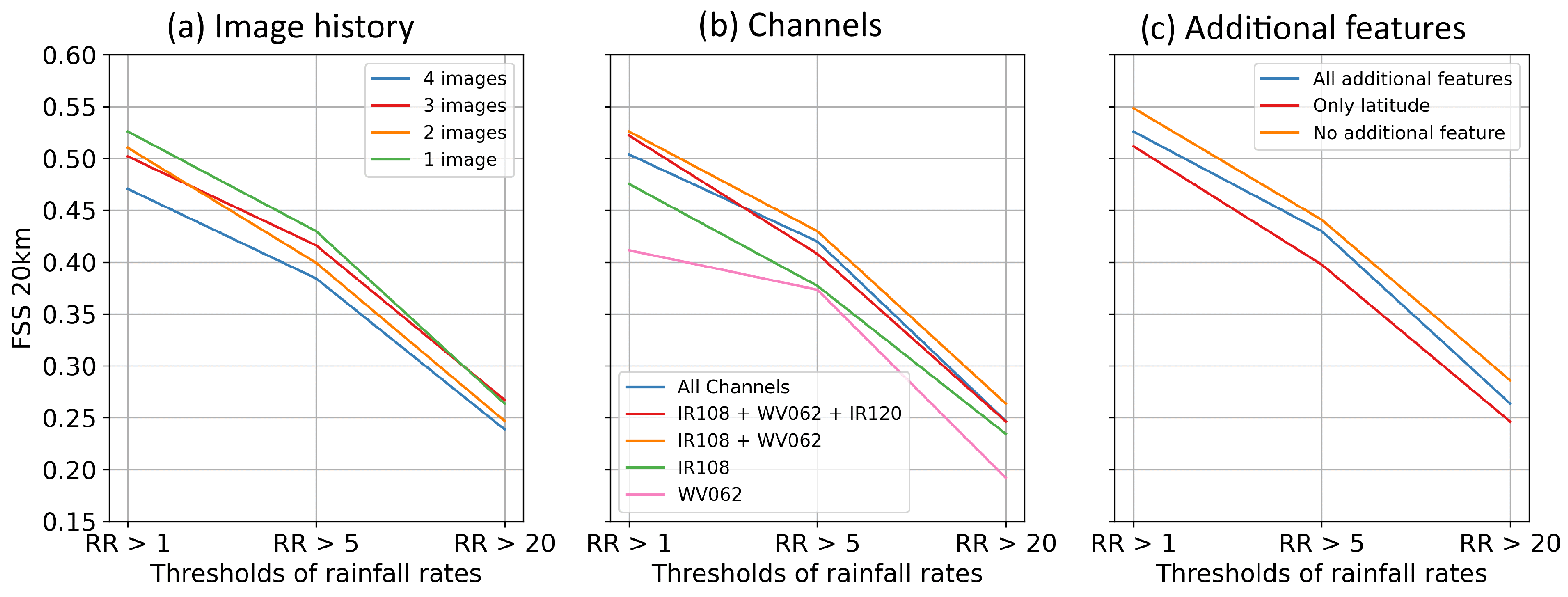
First, we evaluated the effect of varying the number of GEO images used as the input. Figure 4a illustrates the performance of the model when varying the number of input images. Interestingly, using only the most recent image resulted in an improved FSS for the precipitation estimation. As depicted in the figure, the model’s performance improved as the historical images were removed, although the performance does not strictly follow the number of images. This indicates that the most recent image provides the most relevant information for estimating the current precipitation. Including additional images introduces either noise or redundant information.

Next, we investigated the influence of different channels on the model’s performance. Figure 4b provides valuable insights into the significance of channel selection. Firstly, it demonstrates that combining the IR108 channel with WV062 significantly enhanced the FSS score across all the rain rate thresholds, compared to using either of these channels alone. Secondly, adding channels such as VIS006 and IR120 did not significantly improve the model’s FSS and, in fact, resulted in a degraded score. Similar to the historical series of images, the IR120 and VIS006 channels may only introduce noise or redundant information. These findings suggest that a combination of the IR108 and WV062 channels provides sufficient information for reliable precipitation estimates.

Further, we evaluated the significance of our additional descriptive features, including the latitude, longitude, sun elevation, and date information. The inclusion of these features aimed to enhance the model’s capacity to generalize across various regions and climates. We trained the model three times: once with all the additional features, once with only the latitude feature, and finally without any additional features. Figure 4c shows that incorporating these additional features does not improve the model’s performances but actually degrades them.

These findings contradict our initial assumption that more features would help the network generalize to different situations and enhance its performance. Our hypothesis is that these additional sources of information are not relevant and the variability in the model’s performance is more due to intrinsic variability in the initialization of the weights and the training process than to the addition of features. Consequently, we determined the optimal configuration for the precipitation estimation model: our final configuration, named Espresso, focuses solely on the most relevant information, utilizing only the most recent GEO image as input, combined with the IR108 and WV062 channels. This is the configuration that was used in the subsequent experiments.

3.2. Evaluation of Espresso on the Test Set

Having established the optimal configuration for the Espresso model, its performances against the test set of the GPMCO data were evaluated. The evaluation provides insights into the model’s accuracy and its ability to estimate precipitation effectively.

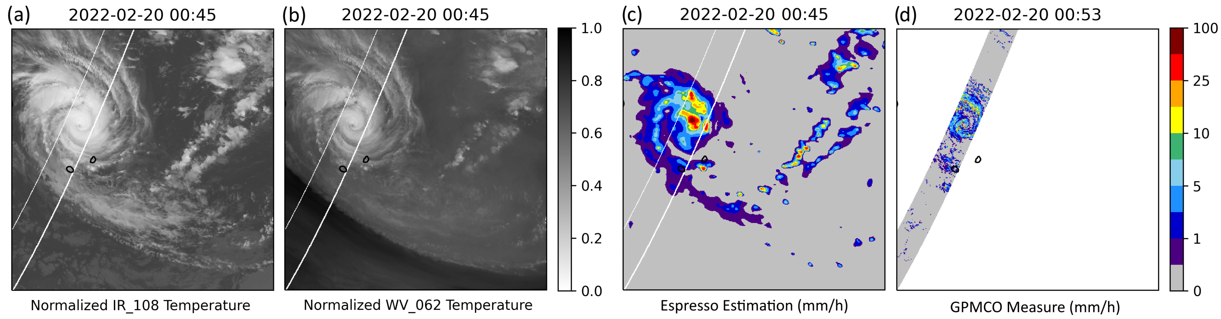
The evaluation begins with an example of rainfall estimation from Espresso. Figure 5 depicts the case of cyclone Emnati, which developed into a category 4 tropical cyclone when it passed north of La Réunion and Mauritius on the 20 September 2022. The cyclone caused flooding and wind gusts at speeds of 163 km/h recorded at the Maido station in La Réunion. The figure shows the two channels used as input for the neural network (IR108 and WV062), the estimation from Espresso, and the GPMCO rainfall measure. The comparison between Espresso and the GPMCO reveals certain characteristics. The rainfall field appears more smoothed and spread out compared to the data from the GPMCO. As a result, the spatial precision of Espresso is not as refined as that of the GPMCO, and it overlooks some light rains in the north and south of the GPM swath. Moreover, Espresso tends to enlarge the area’s rainfall, resulting in a consistent overestimation of precipitation within and on the fringes of rain cells. This characteristic can be attributed to the nature of the deep learning regression model trained with the MSE, which is unable to generate data as precise and discontinuous as the GPMCO’s. However, Espresso effectively captures the structure of the cyclone, including the eye wall with its peak rainfall intensity and the surrounding rainbands. The cyclone is well-positioned, and the intense rainfalls associated with the cyclone are accurately represented.

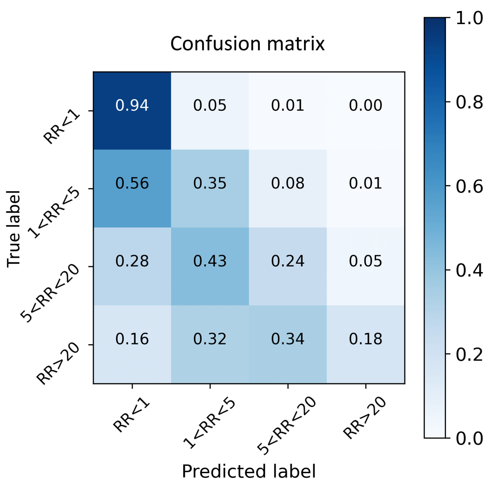
Secondly, Figure 6 showcases the confusion matrix, providing a comprehensive view of the model’s ability to correctly classify rainfall intensities. It is evident from the figure that the model demonstrates strong performance in accurately identifying the “No Rain” category. However, its accuracy diminishes for higher rainfall thresholds, often resulting in an underestimation of precipitation rates. For instance, more than half of the “light rain” cases are mistakenly classified as “No rain”. Meanwhile, the model overlooks fewer medium and heavy rainfalls cases, still detecting some rain in the majority of cases, even if it is underestimated.

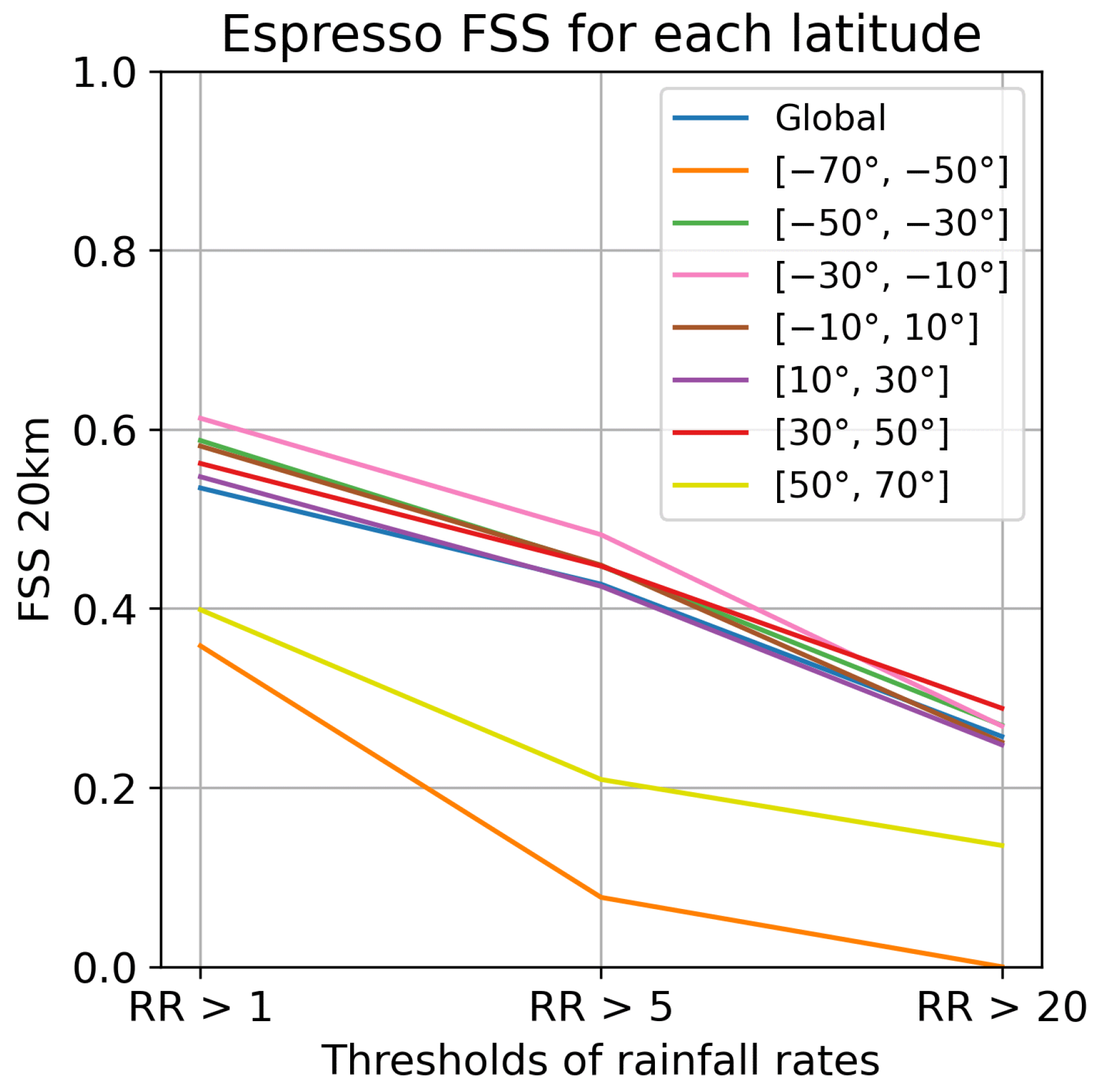
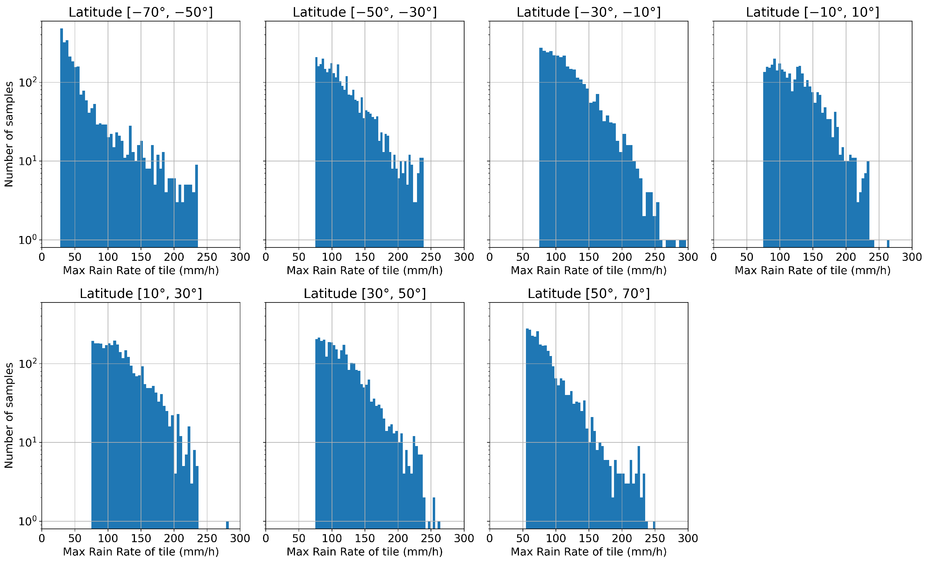
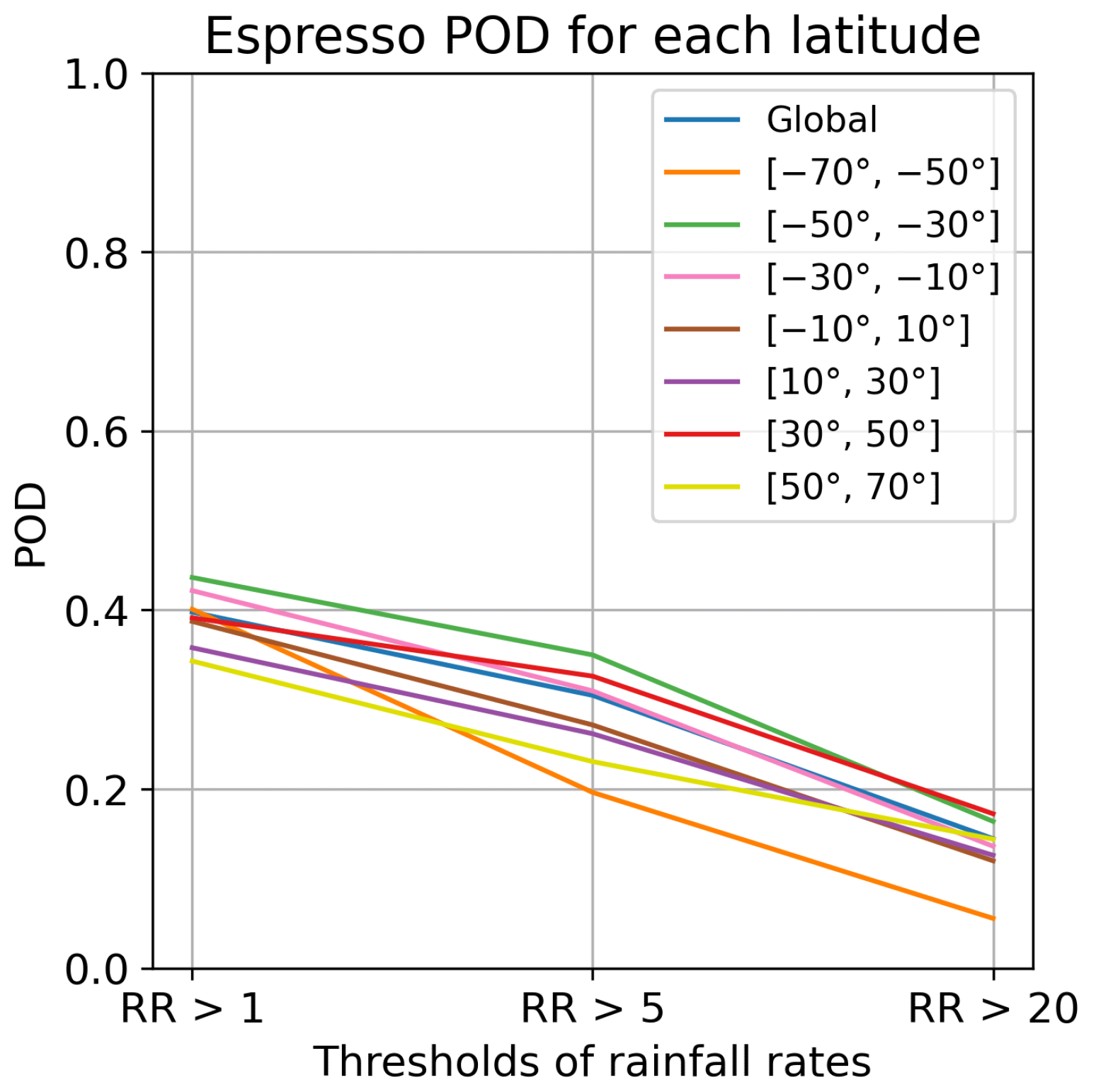
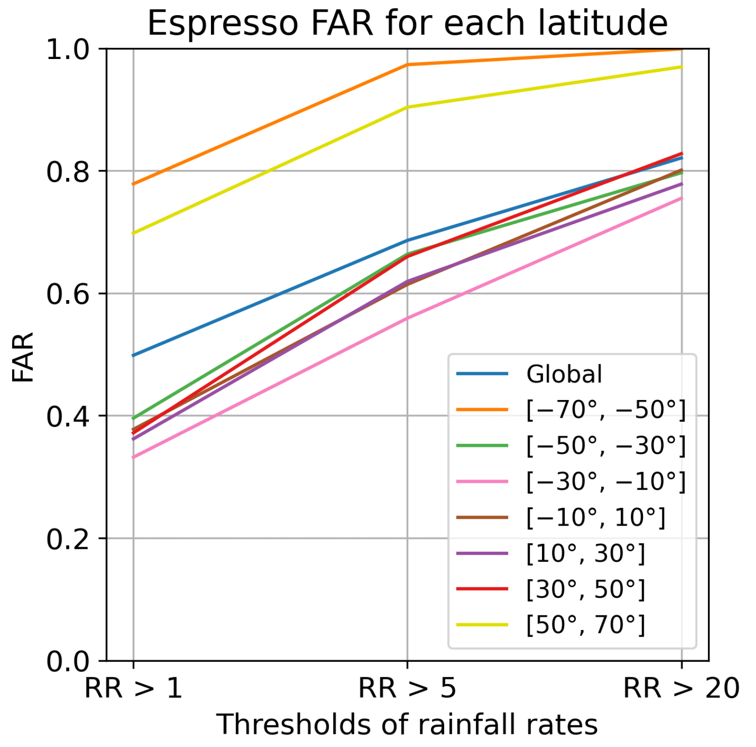
To further assess the model’s performance, we calculated the Fraction Skill Score (FSS), Probability of Detection (POD), and False Alarm Rate (FAR) of Espresso on the test set. Figure 7 gives an overview of the FSS across various latitudes. Across each latitude band, the FSS decreases as the rainfall threshold increases, reflecting the trends observed in the confusion matrix accuracy. This characteristic can be attributed to the neural network’s challenge in generalizing infrequent events not extensively represented in its training dataset. Additionally, as observed in Figure 5, the model tends to smooth the finer details present in the GPMCO, occasionally leading to the omission of isolated, intense rainfall pixels.

Furthermore, the model shows its best performance near the equator, with a higher FSS for all three rain thresholds. On the other hand, the FSS on the [−70${}^{°}$; −50${}^{°}$] and [50${}^{°}$; 70${}^{°}$] bands of latitude range from poor to very poor for heavy rainfalls. The POD and FAR, available in Appendix C, support the same conclusions, even if the difference between the POD near the poles and at the equator is less marked.

These results suggest that while the model is able to accurately detect and estimate precipitation in temperate and tropical regions, it struggles to do so at higher latitudes. Despite precautions to oversample the dataset and weigh the loss in the higher latitudes, heavy rainfalls in these regions are still too scarce to allow the network to learn the different patterns of rain near the poles. In addition, at the poles, the tropopause is lower and the angle between the ground and the satellite’s sensors is greater, leading to a diminished contrast between precipitating and non-precipitating clouds. This makes the task of rain detection more challenging, even to the human eye. Moreover, it is worth noting that the overall FSS, POD, and FAR scores for each latitude band are relatively low. The significant variations in precipitation between adjacent pixels due to localized phenomena pose difficulties for a deep learning model to accurately reproduce, as seen in Figure 5.

These results, based on the 2022 GPMCO data, underscore Espresso’s ability to effectively estimate precipitation across a range of rainfall categories in temperate and tropical regions. Nearer to the poles it often overlooks rainfall, especially heavy rainfalls. Although the model cannot reproduce the fine details of the GPMCO data, as evident from Figure 5, it may still prove useful to forecasters in situations of extreme rainfall.

3.3. Comparison with Other Operational Products

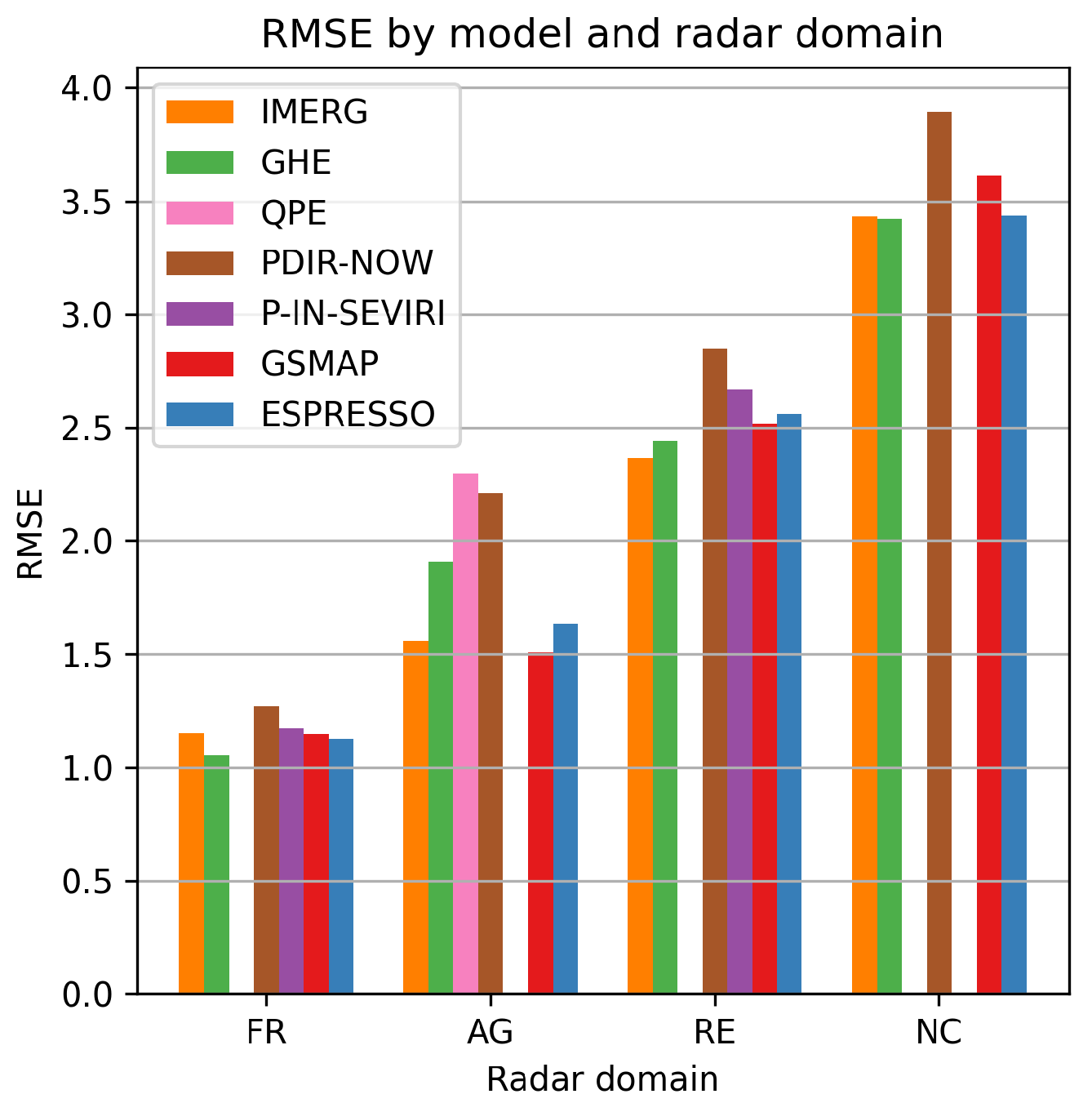
In order to thoroughly evaluate the Espresso model, we carried out a comparative analysis against six other operational precipitation estimation products: IMERG, GHE, QPE, PDIR-NOW, P-IN-SEVIRI, and GSMAP. This evaluation concentrated on 1000 samples of 1 h accumulated data from 2022, spanning across our four radar domains. It is worth noting that QPE and P-IN-SEVIRI are generated in a geostationary space view; thus, they are not available across all the French radar domains.

Figure 8 presents the RMSE of each product across each radar domain. The overall RMSE values are higher in the tropical domains, which experience heavier rainfall than mainland France, leading to larger errors for all the models. Espresso is comparable to the other models, with IMERG, GSMAP, and PDIR-NOW competing for the lowest RMSE. The error of Espresso against ground radar data is on par with the other models. However, the RMSE does not provide information about the distributions of these errors.

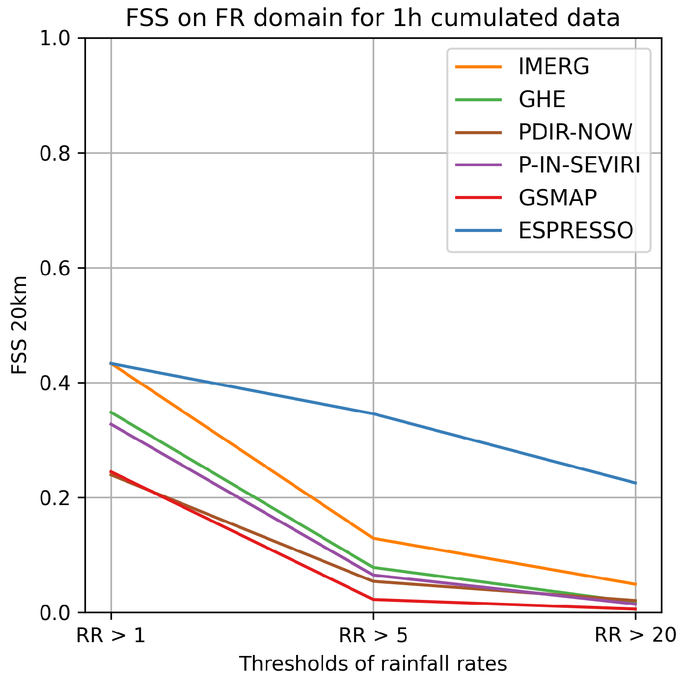
Next, we examined the FSS, POD, and FAR. Figure 9 displays the FSS for the France domain for each model. The FSS for the other domains, along with the POD and FAR for each domain, can be found in Appendix D.1 and Appendix D.2.

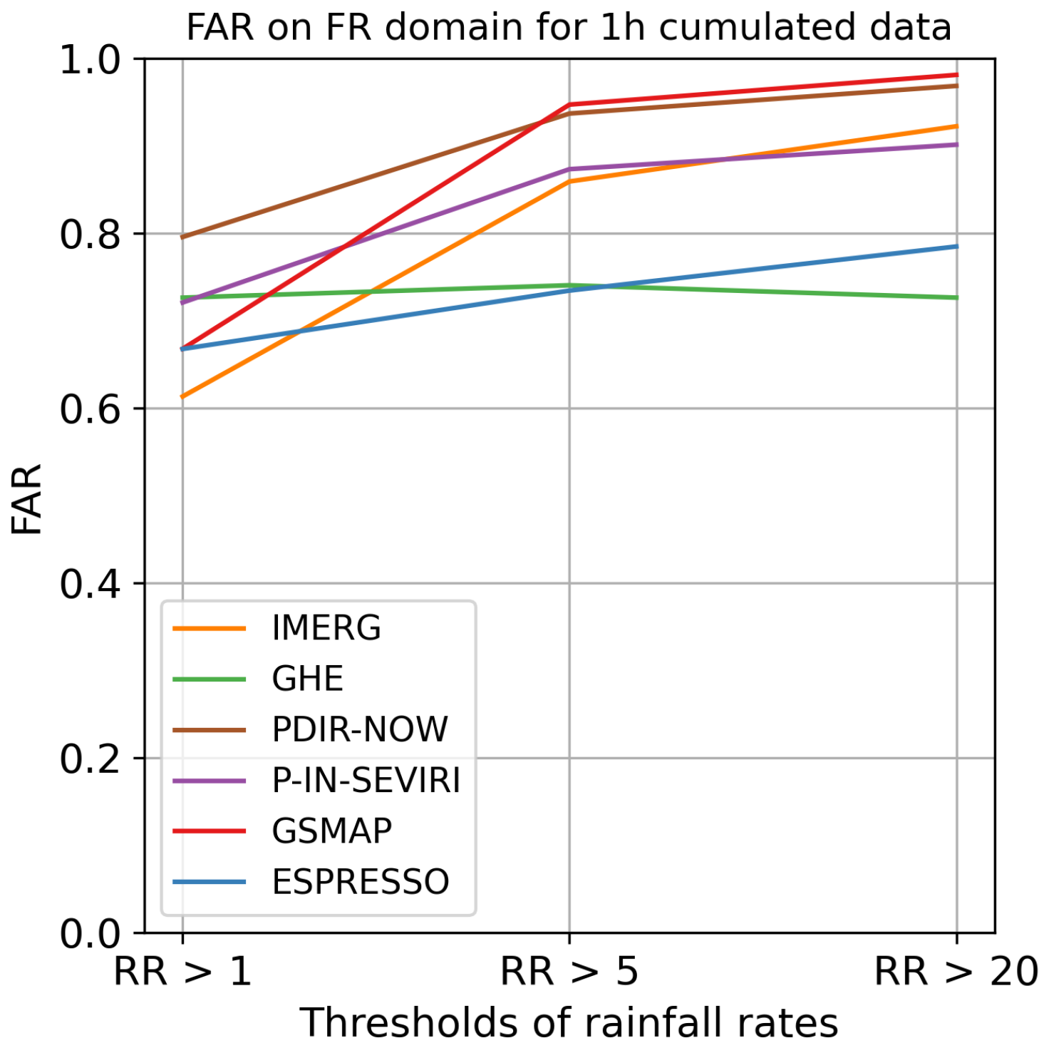
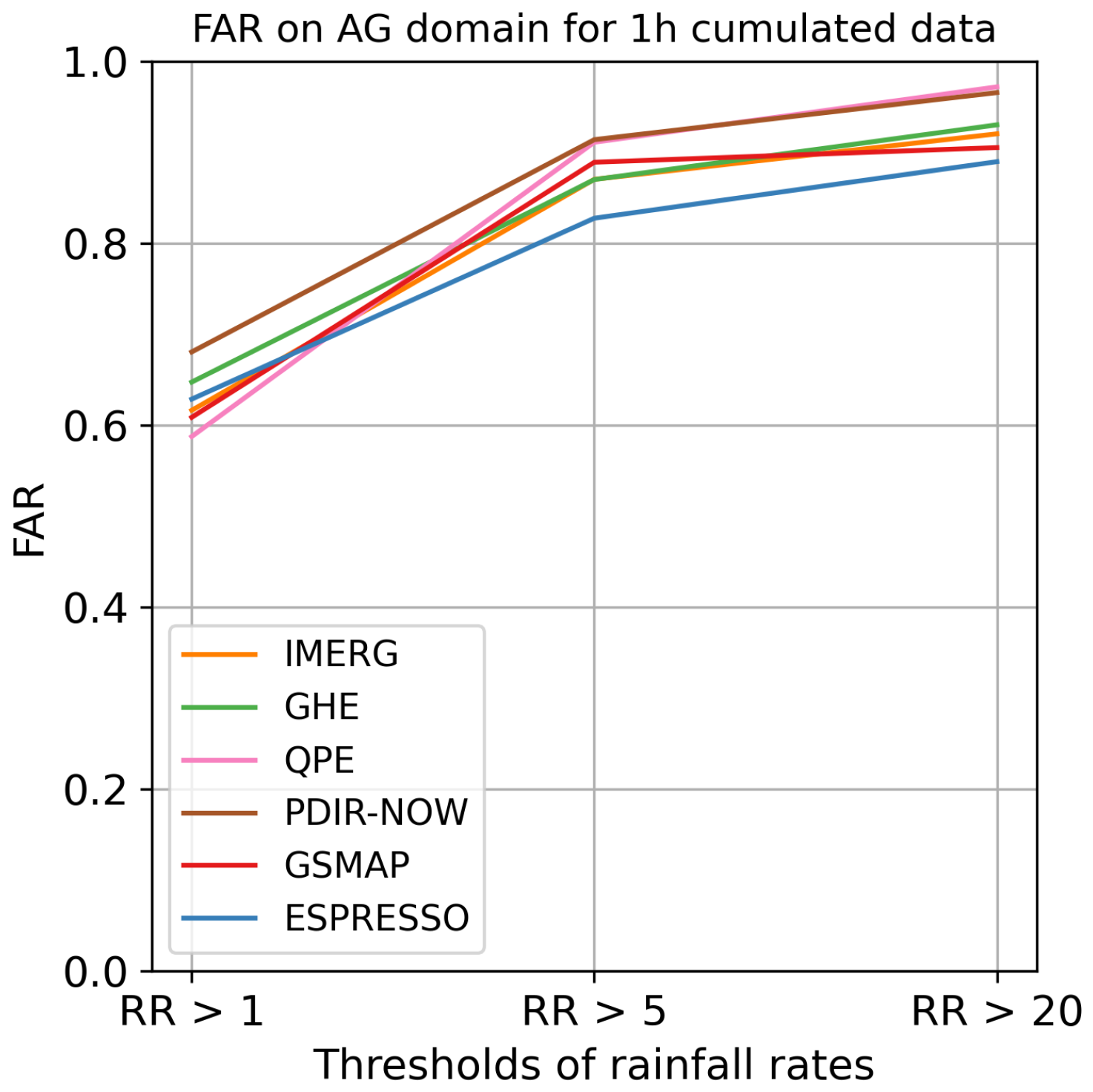
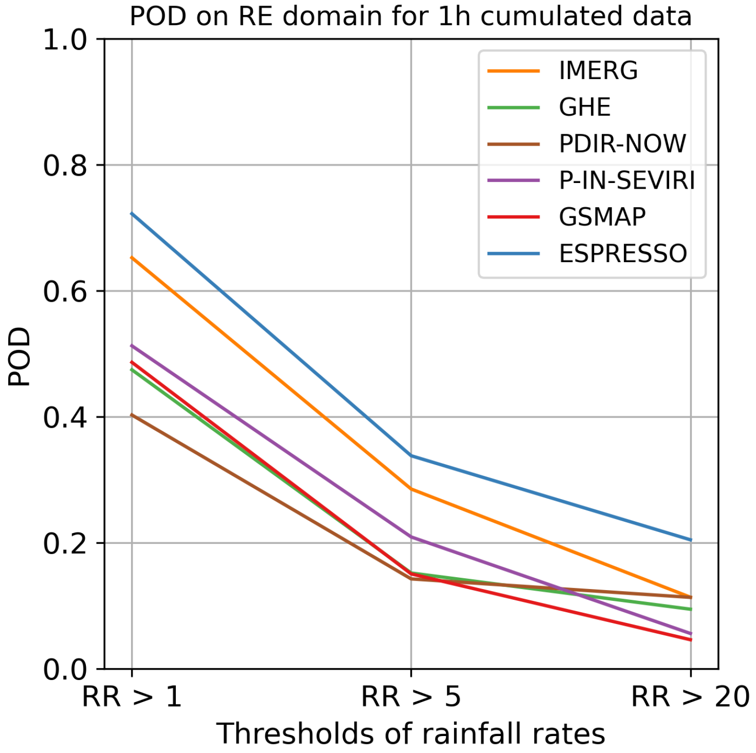
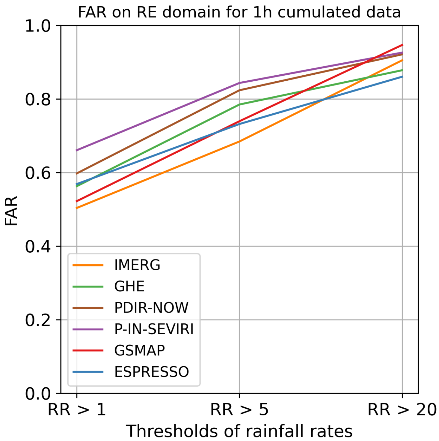
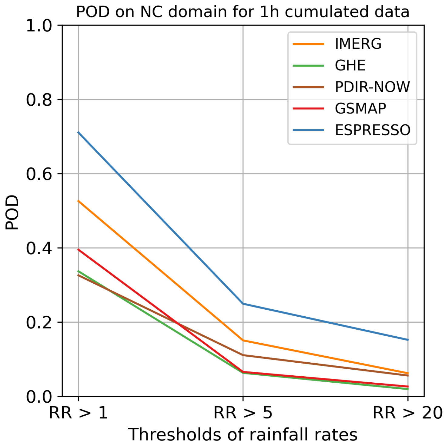
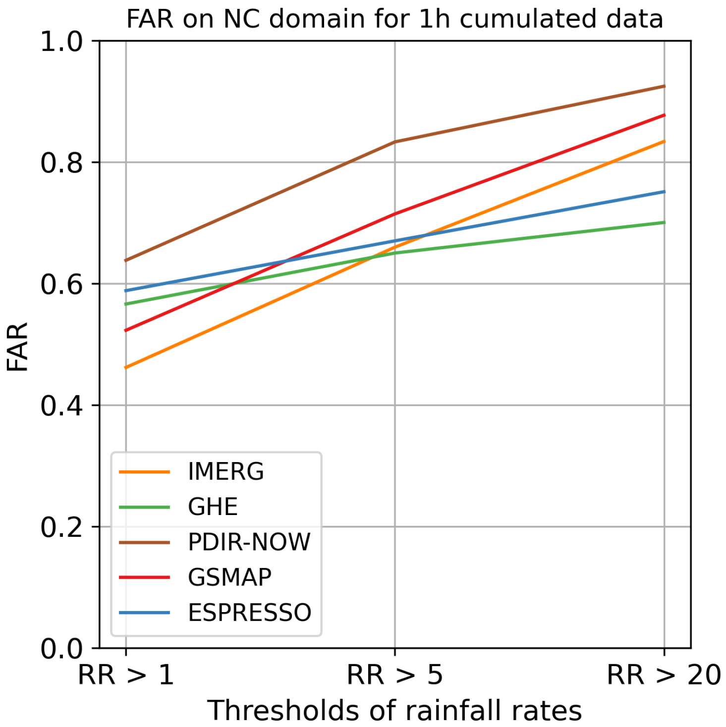
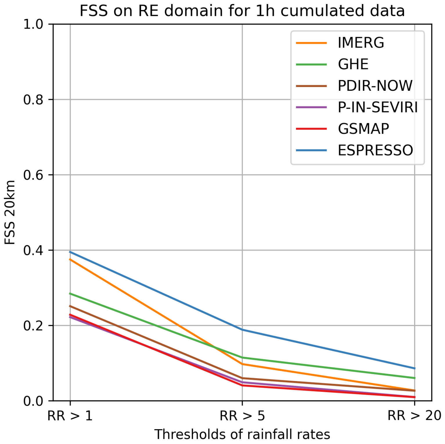
Espresso demonstrates superior performance in the FR, NC, and RE domains, achieving higher scores in terms of the FSS and POD compared to the other models. IMERG trails Espresso in performance, while the rest of the models exhibit comparable quality to each other but fall short of Espresso and IMERG. However, when all the domains are taken into account, Espresso is outpaced by IMERG and occasionally GSMAP and GHE in terms of the FAR for weak and moderate rainfall. Nonetheless, Espresso exhibits a lower FAR for heavy rainfall than IMERG and GSMAP, but on the NC and FR domains, Espresso is bested by GHE for heavy rainfall events.

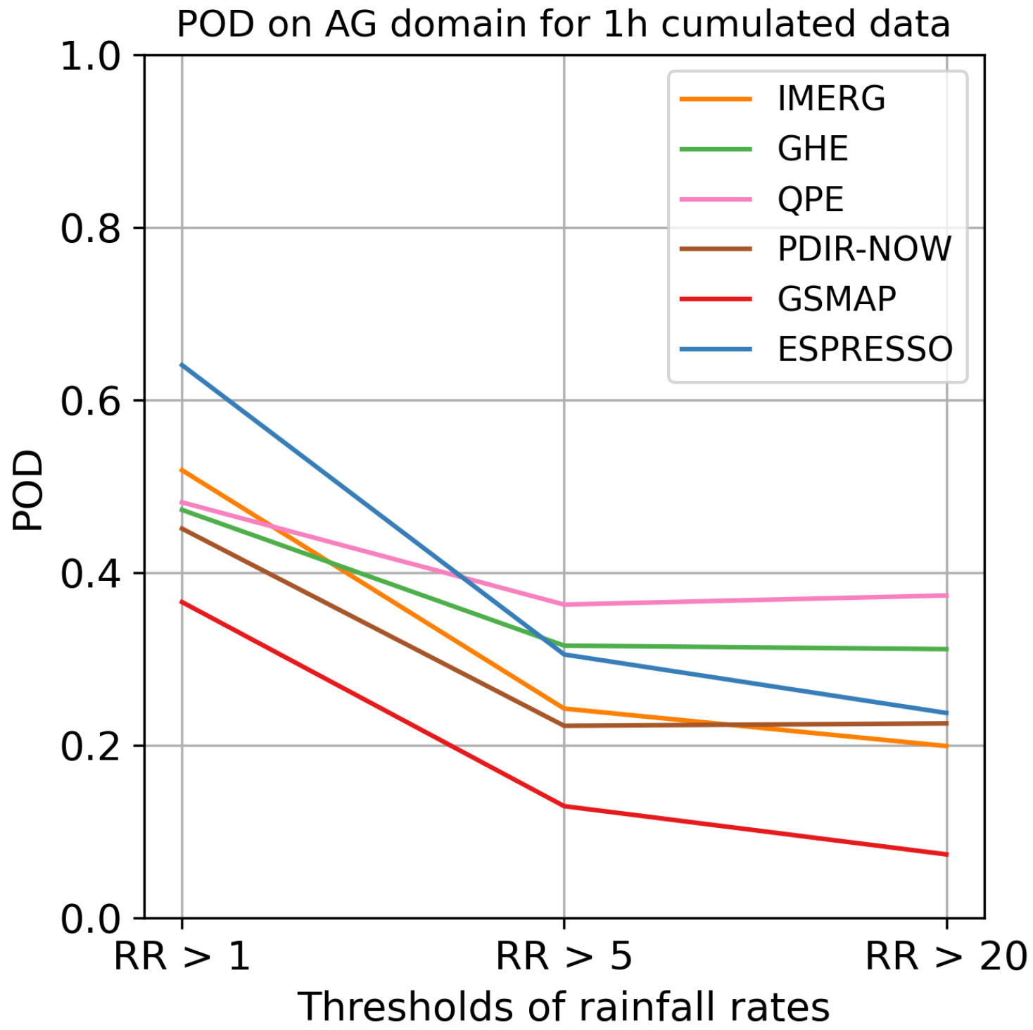
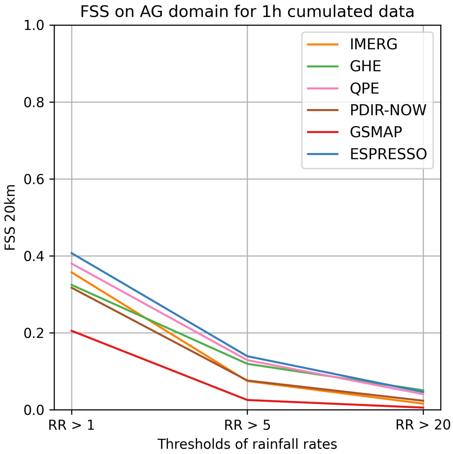
In the AG domain, the GHE and QPE models outperform IMERG in terms of the FSS and POD. While Espresso maintains its superiority in terms of the FSS, it is significantly outdone by GHE and QPE in the detection of moderate and heavy rainfall. Among the global models, Espresso outperforms the rest in nearly all the FSS and POD scores, particularly in heavy precipitation events.

These results establish that Espresso is better at detecting and localizing rainfall than the other global products, especially heavy rainfall. It demonstrates a superior POD and FSS across all four domains with distinct climates. Simultaneously, its FAR is comparable to other products, indicating that Espresso does not overestimate rainfall and can be used in crisis management. The less pronounced difference with the other products in terms of the FAR and RMSE can be explained by the model’s intrinsic spreading of precipitation, which causes false alarms on the periphery of precipitation cells.

These findings position Espresso as a viable and reliable alternative to existing operational products for precipitation estimation. Espresso delivers real-time, accurate, and efficient precipitation estimates, comparable to or better than the widely recognized IMERG, without the associated data availability time delays.

3.4. Case Study

To further assess the Espresso model’s performance and visually compare it to the other six operational products, Météo-France forecasters conducted a double-blind review involving 15 instances of extreme precipitation events. Where available, their assessments were made in reference to radar readings and rain gauge measurements. The evaluation criteria included the maximum rainfall captured by the radar and predicted by the various models, the spatial distribution and spread of rainfall, and the structural representation of the event.

Overall, the forecasters exhibit a preference for Espresso, primarily due to its superior ability in localizing events and the proximity of its estimations to actual rain gauge values. GHE is the next preferred model due to its ability to accurately locate rainfall, even though the estimations are somewhat underestimated. IMERG, QPE, PDIR-NOW, and P-IN-SEVIRI are regarded similarly, with the precipitation cells often mislocated and underestimated. In contrast, GSMAP is least preferred as it frequently failed to detect precipitation events altogether. However, all the products tend to produce structures larger than the actual events.

Below, the analysis of two specific cases is detailed: one in Montpellier, located in the south of mainland France, along the Mediterranean coast, and another in the island of Guadeloupe.

3.4.1. Case Study 1: Stationary Convective Storm in Montpellier

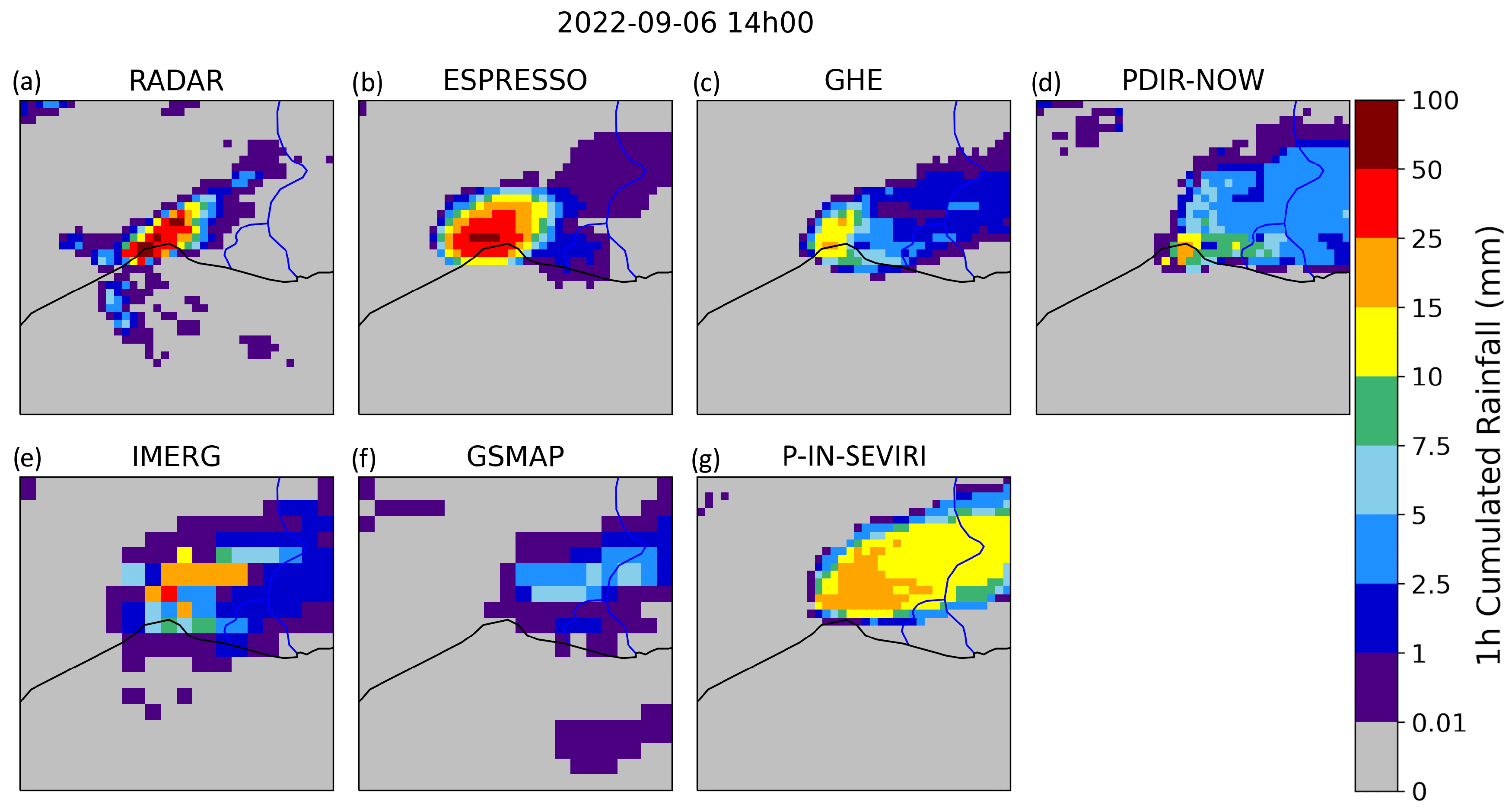
The first case study features a stationary convective storm that impacted Montpellier on 6 September 2022, leading to a meteorological warning due to flooding risks and potential river overflow. This storm caused substantial rainfall, accumulating up to 70 mm in a single afternoon. Figure 10 displays the 1 h cumulative estimations from each of the six available models, as well as the ground radar’s estimation.

Upon analysis, it was observed that GSMAP failed to detect the storm, perceiving only light rainfall. While the other operational products successfully pinpointed the storm, they consistently underestimated the associated rainfall. In contrast, Espresso emerged as the superior model in this scenario, accurately identifying and locating the storm and providing reliable rainfall estimates.

These results underscore the robustness and effectiveness of the Espresso model in capturing the detailed features of convective storms and providing accurate precipitation estimates. Figure 10 also highlights Espresso’s excellent spatial resolution (5 km), which is comparable to GHE, PDIR-NOW, and P-IN-SEVIRI and notably superior to IMERG and GSMAP (10 km).

3.4.2. Case Study 2: Southeast Flow over Guadeloupe Island

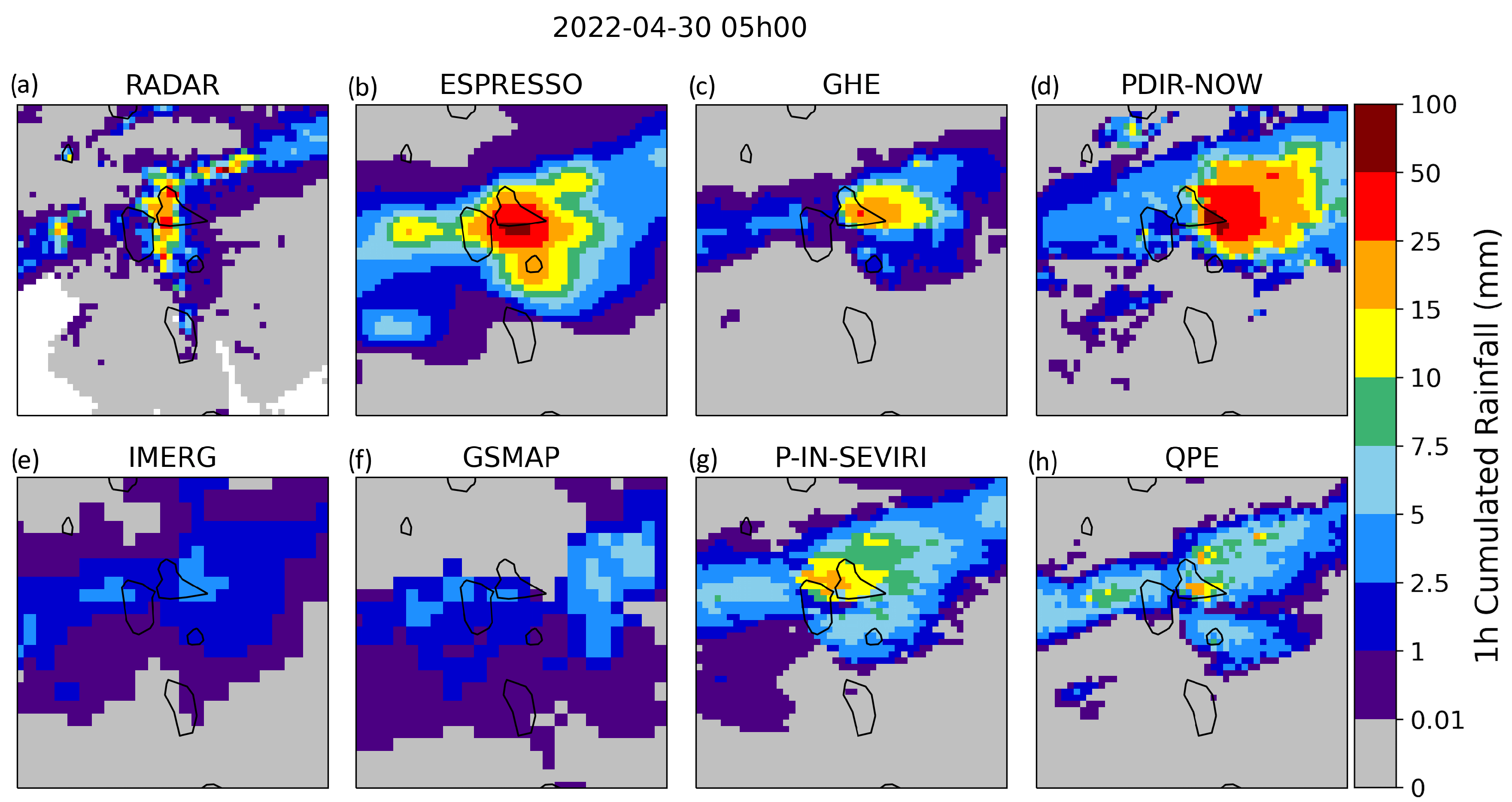
Our second case study focuses on a southeast airflow over Guadeloupe island, characterized by warm and humid air. The combination of converging low-level winds, wind shear at higher altitudes, and the unique configuration of the island amplified the convective activity. Consequently, the region witnessed heavy rainfall, resulting in widespread flooding and the issuance of a meteorological warning. Record-breaking precipitation levels were noted, especially at the Raizet station, where 312 mm fell within a 24 h period. This severe rainfall event caused substantial material damage and fatalities. Figure 11 displays the 1 h cumulative estimations from each of the six available models, as well as the ground radar’s estimation.

Upon evaluating the performance of the operational products in this scenario, we found that both GSMAP and IMERG failed to detect the storm. While GHE, P-IN-SEVIRI, and QPE were successful in pinpointing the storm’s location, they consistently underestimated its intensity. On the other hand, both Espresso and PDIR-NOW exhibited remarkable proficiency in storm localization and intensity estimation. Their ability to accurately locate and estimate extreme rainfall values highlights their potential for providing invaluable data for disaster management and response initiatives.

In conclusion, the Montpellier and Guadeloupe case studies consolidate Espresso’s position as a reliable and capable model for precipitation estimation. Despite its tendency to overestimate precipitation within and on the periphery of rain cells, the model’s demonstrated accuracy in localizing and estimating the intensity of convective storms underscores its practical utility in real-time monitoring and response to extreme weather events.

3.5. Computational Resources

The training of each experiment was performed on four Nvidia Tesla V100 Graphical Processing Units (GPU) and took approximately 4 h for the neural network to converge. Over the course of this year-and-a-half-long research project, a total of 160 training experiments were conducted. This accumulates to a total computation time of 27 days, equivalent to an electricity consumption of 650 kWh.

On the other hand, the inference phase, which covers the entire globe, requires only around 5 min of computation time on a single Central Processing Unit (CPU).

4. Discussion

Throughout this work, we have presented the development and evaluation of Espresso, a convolutional neural network architecture that leverages satellite imagery for global precipitation estimation. As a global model, Espresso overcomes the limitations of data availability delays inherent to operational models such as IMERG, offering real-time precipitation estimates while maintaining or even exceeding the performance of existing operational products. Furthermore, the relatively low computational cost of the inference phase and ease of deployment add to the model’s appeal, making it an attractive solution for operational use.

The model has been carefully designed to ensure that the high resolution of the input satellite data is preserved, contributing to the precise detection and estimation of precipitation events. In the various evaluations conducted, Espresso has demonstrated its ability to accurately capture precipitation patterns across the globe, particularly in temperate and tropical regions. It provides a better POD and FSS, and a similar FAR, when compared to other models, especially for heavy rainfall.

However, the model’s performance was found to be less robust at higher latitudes, an aspect that could be improved in future iterations. While the current approach to addressing the imbalance in the data using oversampling and weighting the loss has proven to be somewhat effective, other methods could be explored to further improve the model’s ability to learn in these regions. One potential solution is to incorporate data from periods before 2018 and after 2022.

Additionally, advancements in deep learning architectures such as Vision Transformers [35] and diffusion models [36] could be utilized to develop a model that provides finer details than our DeepLabV3+ and lowers the False Alarm Rate of the model. Furthermore, enhancements in the infrared sensors of the next generation of satellites, such as Meteosat Third Generation, are anticipated to yield higher-resolution infrared GEO images, thereby contributing to improved estimation accuracy.

Furthermore, our attempt to enhance the model’s performance by incorporating additional features like topography, latitude, or season into additional channels has proven to be ineffective. Better results might be achieved by adopting an approach similar to the recent MetNet-3 [37], where the authors prefer to use topographical embeddings. This allows the network to autonomously discover relevant topographical information and store it in the embedding. This embedding is a trainable parameter, similar to techniques used in Natural Language Processing. Additionally, the seasonal information, which is constant for a single sample or for a global inference, could be integrated into the output of the final encoder layer prior to the first decoder layer. By adopting this approach, the model might be able to make more effective use of this information, as it would be connected to the features already learned from the input image.

5. Conclusions

In conclusion, this paper presents Espresso, a deep convolutional neural network designed for global precipitation estimation using satellite data. The model has demonstrated strong performance across various geographical regions, particularly in temperate and tropical zones. The ability of Espresso to detect and accurately estimate rainfall, especially heavy rainfall, establishes it as a reliable and competitive tool in the field of weather prediction and monitoring.

Despite some limitations in higher latitudes, the model demonstrates significant results and potential for further improvements. Future work could explore new approaches to address the imbalance in the data, incorporate additional data sources, or fine-tune the model parameters to enhance performance. As weather patterns continue to become increasingly complex due to climate change, the role of precise, real-time precipitation estimation models like Espresso becomes critical.

Espresso has been incorporated as an operational product at Météo-France, delivering high-quality, real-time global precipitation estimates every 30 min. These estimations are readily accessible to forecasters for monitoring French Overseas Territories, where ground radars may not be available, and for anticipating the movement of incoming precipitation before it becomes visible on radars. This tool strengthens Météo-France’s ability to respond to and manage the impacts of extreme weather events, thereby contributing to the protection of people and property across French territories.

References

1. Tropical Globe’s Database of Publicly Accessible Weather Radars. Available online: http://tropicalglobe.com/radar_database/list.shtml (accessed on 19 July 2023).
2. Prigent, C. Precipitation retrieval from space: An overview. Comptes Rendus Geosci. 2010, 342, 380–389. [Google Scholar] [CrossRef]
3. Adler, R.; Braun, S.; Stocker, E.; Marius, J. Tropical Rainfall Measuring Mission, TRMM, Senior Review Proposal; Technical Report; Laboratory for Atmospheres, NASA Goddard Space Flight Centre: Greenbelt, MD, USA, 2007.
4. Smith, E.A.; Asrar, G.; Furuhama, Y.; Ginati, A.; Mugnai, A.; Nakamura, K.; Zhang, W. International global precipitation measurement (GPM) program and mission: An overview. In Measuring Precipitation from Space: EURAINSAT and the Future; Springer: Dordrecht, The Netherlands, 2007; pp. 611–653. [Google Scholar]
5. NOAA, Office of Satellite and Product Operations. Global Hydro-Estimator—Algorithm Description. Available online: https://www.ospo.noaa.gov/Products/atmosphere/ghe/algo.html (accessed on 19 July 2023).
6. Nguyen, P.; Ombadi, M.; Gorooh, V.A.; Shearer, E.J.; Sadeghi, M.; Sorooshian, S.; Ralph, M.F. Persiann dynamic infrared–rain rate (PDIR-now): A near-real-time, quasi-global satellite precipitation dataset. J. Hydrometeorol. 2020, 21, 2893–2906. [Google Scholar] [CrossRef] [PubMed]
7. NOAA NESDIS Center for Satellite Applications and Research. GOES-R Advanced Baseline Imager (ABI) Algorithm Theoretical Basis Document For Rainfall Rate (QPE). Available online: https://www.star.nesdis.noaa.gov/goesr/documents/ATBDs/Enterprise/ATBD_Enterprise_Rainfall_Rate_v3_2020-07-10.pdf (accessed on 19 July 2023).
8. EUMETSAT HSAF. Algorithm Theoretical Baseline Document (ATBD) for Product H03B—P-IN-GRU-SEVIRI. Precipitation Rate at Ground by GEO/IR Supported by LEO/MW; Technical Report; EUMETSAT: Darmstadt, Germany, 2017. [Google Scholar]
9. Kuligowski, R.J. The Self-Calibrating Multivariate Precipitation Retrieval (SCaMPR) for high-resolution, low-latency satellite-based rainfall estimates. In Satellite Rainfall Applications for Surface Hydrology; Springer: Dordrecht, The Netherlands, 2010; pp. 39–48. [Google Scholar]
10. Turk, F.J.; Rohaly, G.; Hawkins, J.D.; Smith, E.A.; Grose, A.; Marzano, F.S.; Levizzani, V. Analysis and assimilation of rainfall from blended SSM/I, TRMM and geostationary satellite data. In Proceedings of the 10th Conference Satellite Meteorology and Oceanography, Long Beach, CA, USA, 9–14 January 2000; pp. 66–69. [Google Scholar]
11. Kubota, T.; Aonashi, K.; Ushio, T.; Shige, S.; Takayabu, Y.N.; Kachi, M.; Arai, Y.; Tashima, T.; Masaki, T.; Kawamoto, N.; et al. Global Satellite Mapping of Precipitation (GSMaP) products in the GPM era. In Satellite Precipitation Measurement; Springer: Cham, Switzerland, 2020. [Google Scholar]
12. NASA Global Precipitation Measurement (GPM) Integrated Multi-satellitE Retrievals for GPM (IMERG). Algorithm Theoretical Basis Document (ATBD) Version 06. 2020. Available online: https://gpm.nasa.gov/sites/default/files/2020-05/IMERG_ATBD_V06.3.pdf (accessed on 19 July 2023).
13. Pritt, M.; Chern, G. Satellite image classification with deep learning. In Proceedings of the 2017 IEEE Applied Imagery Pattern Recognition Workshop (AIPR), Washington, DC, USA, 10–12 October 2017; pp. 1–7. [Google Scholar]
14. Jeppesen, J.H.; Jacobsen, R.H.; Inceoglu, F.; Toftegaard, T.S. A cloud detection algorithm for satellite imagery based on deep learning. Remote Sens. Environ. 2019, 229, 247–259. [Google Scholar] [CrossRef]
15. Neupane, B.; Horanont, T.; Aryal, J. Deep learning-based semantic segmentation of urban features in satellite images: A review and meta-analysis. Remote Sens. 2021, 13, 808. [Google Scholar] [CrossRef]
16. Tao, Y.; Hsu, K.; Ihler, A.; Gao, X.; Sorooshian, S. A two-stage deep neural network framework for precipitation estimation from bispectral satellite information. J. Hydrometeorol. 2018, 19, 393–408. [Google Scholar] [CrossRef]
17. Sadeghi, M.; Asanjan, A.A.; Faridzad, M.; Nguyen, P.; Hsu, K.; Sorooshian, S.; Braithwaite, D. PERSIANN-CNN: Precipitation estimation from remotely sensed information using artificial neural networks–convolutional neural networks. J. Hydrometeorol. 2019, 20, 2273–2289. [Google Scholar] [CrossRef]
18. Wang, C.; Xu, J.; Tang, G.; Yang, Y.; Hong, Y. Infrared precipitation estimation using convolutional neural network. IEEE Trans. Geosci. Remote Sens. 2020, 58, 8612–8625. [Google Scholar] [CrossRef]
19. Hayatbini, N.; Kong, B.; Hsu, K.L.; Nguyen, P.; Sorooshian, S.; Stephens, G.; Ganguly, S. Conditional generative adversarial networks (cGANs) for near real-time precipitation estimation from multispectral GOES-16 satellite imageries—PERSIANN-cGAN. Remote Sens. 2019, 11, 2193. [Google Scholar] [CrossRef]
20. Chen, H.; Chandrasekar, V.; Cifelli, R.; Xie, P. A machine learning system for precipitation estimation using satellite and ground radar network observations. IEEE Trans. Geosci. Remote Sens. 2019, 58, 982–994. [Google Scholar] [CrossRef]
21. Wang, C.; Tang, G.; Gentine, P. PrecipGAN: Merging microwave and infrared data for satellite precipitation estimation using generative adversarial network. Geophys. Res. Lett. 2021, 48, e2020GL092032. [Google Scholar] [CrossRef]
22. Wang, C.; Tang, G.; Xiong, W.; Ma, Z.; Zhu, S. Infrared Precipitation Estimation using Convolutional neural network for FengYun satellites. J. Hydrol. 2021, 603, 127113. [Google Scholar] [CrossRef]
23. Gao, Y.; Guan, J.; Zhang, F.; Wang, X.; Long, Z. Attention-unet-based near-real-time precipitation estimation from fengyun-4A satellite imageries. Remote Sens. 2022, 14, 2925. [Google Scholar] [CrossRef]
24. Olson, W. GPM DPR and GMI Combined Precipitation L2B 1.5 h 5 km V07. 2022. Available online: https://doi.org/10.5067/GPM/DPRGMI/CMB/2B/07 (accessed on 1 April 2023).
25. Huffman, G.; Stocker, E.; Bolvin, D.; Nelkin, E.; Tan, J. GPM IMERG Final Precipitation L3 Half Hourly 0.1 degree × 0.1 degree V06. 2019. Available online: https://doi.org/10.5067/GPM/IMERG/3B-HH/06 (accessed on 1 March 2023).
26. Japan Aerospace Exploration Agency. GSMaP (Hourly). 1998. Available online: https://doi.org/10.57746/EO.01gs73bkt358gfpy92y2qns5e9 (accessed on 1 March 2023).
27. GOES-R Algorithm Working Group; GOES-R Program Office. NOAA GOES-R Series Advanced Baseline Imager (ABI) Level 2 Rainfall Rate/QPE. 2018. Available online: https://doi.org/10.7289/V5W66J21 (accessed on 1 March 2023).
28. NOAA Global Hydro Estimator (GHE). Available online: https://registry.opendata.aws/noaa-ghe (accessed on 1 March 2023).
29. Precipitation Estimation from Remotely Sensed Information Using Artificial Neural Networks—Dynamic Infrared Rain Rate near Real-Time (PDIR-Now). Available online: https://chrsdata.eng.uci.edu/ (accessed on 1 March 2023).
30. Precipitation Rate at Ground by GEO/IR Supported by LEO/MW IODC, P-IN-SEVIRI-E (H63). Available online: https://hsaf.meteoam.it/ (accessed on 1 March 2023).
31. Chen, L.C.; Zhu, Y.; Papandreou, G.; Schroff, F.; Adam, H. Encoder-decoder with atrous separable convolution for semantic image segmentation. In Proceedings of the European Conference on Computer Vision (ECCV), Munich, Germany, 8–14 September 2018; pp. 801–818. [Google Scholar]
32. Ronneberger, O.; Fischer, P.; Brox, T. U-net: Convolutional networks for biomedical image segmentation. In Proceedings of the Medical Image Computing and Computer-Assisted Intervention—MICCAI 2015: 18th International Conference, Proceedings, Part III 18, Munich, Germany, 5–9 October 2015; Springer International Publishing: Cham, Switzerland, 2015; pp. 234–241. [Google Scholar]
33. Rakshit, S. Multiclass Semantic Segmentation Using DeepLabV3+. 2021. Available online: https://keras.io/examples/vision/deeplabv3_plus/ (accessed on 1 March 2023).
34. Kingma, D.P.; Ba, J. Adam: A method for stochastic optimization. arXiv 2014, arXiv:1412.6980. [Google Scholar]
35. Hafiz, A.M.; Parah, S.A.; Bhat, R.U.A. Attention mechanisms and deep learning for machine vision: A survey of the state of the art. arXiv 2021, arXiv:2106.07550. [Google Scholar]
36. Yang, L.; Zhang, Z.; Song, Y.; Hong, S.; Xu, R.; Zhao, Y.; Yang, M.H. Diffusion models: A comprehensive survey of methods and applications. arXiv 2022, arXiv:2209.00796. [Google Scholar]
37. Andrychowicz, M.; Espeholt, L.; Li, D.; Merchant, S.; Merose, A.; Zyda, F.; Kalchbrenner, N. Deep Learning for Day Forecasts from Sparse Observations. arXiv 2023, arXiv:2306.06079. [Google Scholar]
Figure 1. Example of a precipitation tile and its associated GEO data on the northern coast of Madagascar: (a) precipitation data from GPMCO in mm/h; (b) normalized albedo of the visible 0.6 µm channel from MSG3; (ce) normalized brightness temperature for the 10.8, 12.0, and 6.2 µm channels, respectively.
Meteorology 02 00025 g001
Figure 2. Radar coverage of our four study areas. (a) Mainland France area (FR); (b) Guadeloupe island area (AG) in the Lesser Antilles archipelago; (c) Réunion island area (RE), east of Madagascar, in the Indian Ocean; (d) New Caledonia islands area (NC) in the South Pacific Ocean.
Meteorology 02 00025 g002
Figure 3. The experimental framework.
Meteorology 02 00025 g003
Figure 4. Fraction Skill Scores for each experiment, as a function of the rainfall rate (RR) in mm/h. (a) Different numbers of input GEO images; (b) number of GEO images set to one, variable GEO input channels; (c) with channels IR108 and WV62, variation in the additional input features.
Meteorology 02 00025 g004
Figure 5. Example of rainfall estimation from Espresso during the cyclone Emnati, north of La Réunion and Mauritius. (a,b) normalized brightness temperature for the 10.8 and 6.2 µm channels, respectively; (c) precipitation estimation from Espresso in mm/h; (d) precipitation data from GPMCO in mm/h.
Meteorology 02 00025 g005
Figure 6. Confusion matrix of the Espresso model for four categories of rainfall rate (RR). True label lines sum to 1.
Meteorology 02 00025 g006
Figure 7. FSS of Espresso for each band of latitude and each threshold of rain.
Meteorology 02 00025 g007
Figure 8. Barplot of the RMSE of each model for each radar domain.
Meteorology 02 00025 g008
Figure 9. Fractions Skill Scores of each model and each threshold of rain, on the mainland France domain.
Meteorology 02 00025 g009
Figure 10. Comparison of the seven models for a convective storm in Montpellier, 6 September 2022. (a) Ground radar data in mm/h; precipitation estimations in mm/h from (b) Espresso, (c) GHE, (d) PDIR-NOW, (e) IMERG, (f) GSMAP, and (g) P-IN-SEVIRI.
Meteorology 02 00025 g010
Figure 11. Comparison of all six models for a case of convective activity in Guadeloupe, 3 April 2022. (a) Ground radar data in mm/h; precipitation estimations in mm/h from (b) Espresso, (c) GHE, (d) PDIR-NOW, (e) IMERG, (f) GSMAP, (g) P-IN-SEVIRI, and (h) QPE.
Meteorology 02 00025 g011