1. Introduction
Regardless of its regional trends, hail represents an extreme weather phenomenon determined by severe convective storms [
1]. Improving the capacity to forecast this weather phenomenon represents one of the main available tools for the mitigation of its impact.
Early hail forecasting methods had limited success, using small statistical samples and developing empirical relationships between hail size and convective available potential energy (CAPE) or temperature values at different levels [
2,
3,
4,
5,
6].
These forecasts used only the available convection energy, estimated either directly from CAPE or indirectly from temperature values at different levels. As a result, these methods tended to forecast unrealistic hail sizes or had poor ability to distinguish between hail formation conditions of small and large dimensions, respectively [
7].
The study results using thermodynamic parameters (closely related to the magnitude of the updraft) were very similar in Europe and in the USA. CAPE or the thermal gradient in the middle troposphere causes the increase in the updraft [
8,
9,
10,
11,
12,
13,
14,
15,
16,
17,
18]. Recent research [
17] has shown that a higher CAPE does not necessarily favour larger hail nor is it a very useful discriminator of size classes [
12,
14,
18]. In Europe, the Lifted Index has been shown to be useful for hail forecasting [
8]. Specialists within the hail control system from the former Soviet republics carried out complex hail forecasting procedures as well. The most important thermodynamic parameters used in operational hail forecasting are those related to: updraft speed, humidity at different levels, and middle tropospheric flow [
19,
20,
21,
22].
Relevant parameters include the vertical gradient of air pressure that cause strong updrafts and hail. These are known as generators of highly organised convective storms. In supercell cases, associated with large-size hailstones, a few parameters have been chosen to help forecast. The wind shear between the surface and the 6 km level (DLS) and the storm’s relative helicity are perhaps the most relevant parameters [
12,
14,
15,
23,
24,
25,
26,
27].
Potential predictors could come from the optimum hail increase zone estimation represented by a layer above the 0 °C isotherm. The rise in the freezing level is used for the same purpose [
12,
28,
29]. The amount of moisture available below the freezing level or in the boundary layer also has an influence on the density and increase rate of hailstones [
12,
29]. Recent research in Europe has suggested that the level of updraft condensation can become a useful predictor [
14,
24,
25] and be correlated with lifting condensation levels, convective temperature, and the cloud base. All these factors influence the speed of the updraft [
30].
Bălescu and Militaru [
31] carried out a study describing favourable convective conditions for hail events. Some studies have addressed the forecast of instability, in general, or of storms using instability indices [
32,
33,
34]. The characterisation of the convective and pre-convective environment of hailstorms appears in case studies of exceptional events [
35,
36]. The efficiency of some instability indices derived from sounding data for hail forecasting was tested on Romanian territory. The Lifted Index, which linked with the values of temperature lapse rate in the middle troposphere, proved a good ability to forecast hail [
37].
Numerous areas with a high hail risk [
38] determined the implementation of hail suppression technologies in the studied area. This study addresses the use of short-term hail forecasting methods in the northeastern part of Romania.
2. Materials and Methods
2.1. Study Area and Hail Climatology
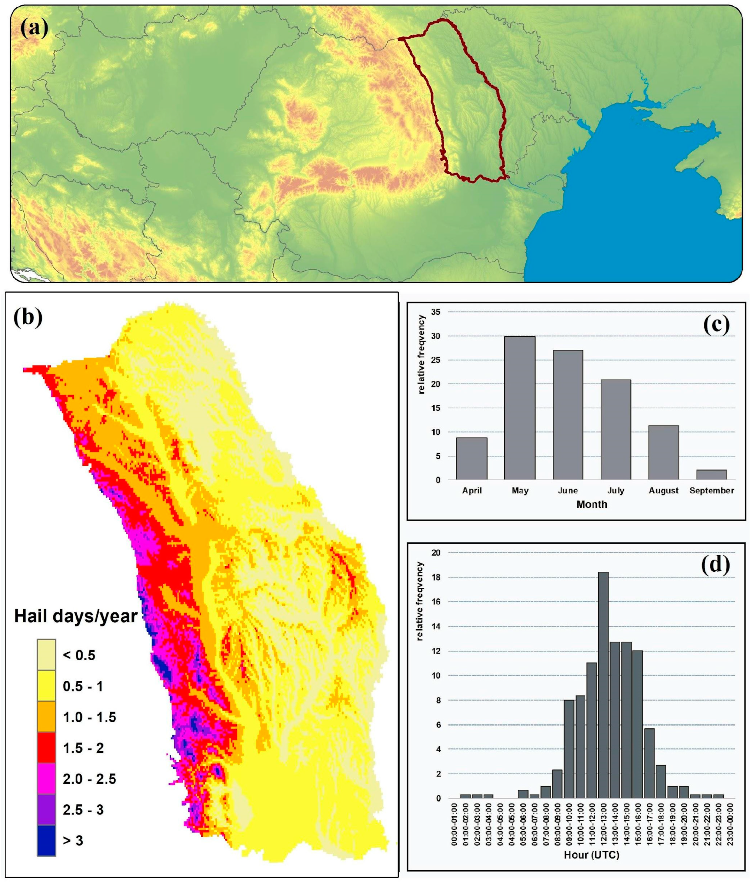
The study is performed in the northeastern part of Romania (
Figure 1a), corresponding with the western part of Moldova’s historical region (
Figure 1b).
The mountain area was excluded due to the lack of significant hail event data. Although the number of days with hail is higher in the mountain area [
39] damage is low due to strong hailstorms [
40]. The studied area hypsometry is between 10 m in the extreme south and over 900 m in the hilly area in the west. The region is sheltered in the western part by the Carpathian Mt., which induces a series of peculiarities [
41].
The mean annual hail frequency drops from 3 days/year on the highest peaks of the Moldavian Subcarpathian and the Curved Subcarpathian, to below 0.6 days/year in the southern Moldavian Plain, the Bârlad valley, and most of the Prut valley [
39]. A total of 78% of hail events occurred in the afternoon and evening hours: between 10:00 and 18:00 UTC, while the rest of the hail events (22%) occur in the interval 19:00–10:00 UTC.
2.2. Hail Data
Data from reported hail events used in this study were used in previous studies [
37,
42], and originate from three different sources: Romanian National Meteorological Administration (RNMA); European Severe Weather Database (ESWD); and the media and local newspapers. If a hailstorm is recorded at one location from the study area on a particular day, we define it as a hail day for this station. The dataset from RNMA contains a total of 242 hail days from 18 weather stations from 1979 to 2017. A total of 29 hail days were taken from ESWD reports, the database used in studies at the continental level [
25,
26,
43,
44] as well as at the regional level [
45]. The third data source is represented by large hail reports from the local newspapers’ archive. These types of meteorological phenomena reports, including data from past centuries, have been used in climatological studies that have been carried out [
46,
47,
48]. The dataset gathered a total of 378 hail days over the studied region.
2.3. Convective Parameters
The convective environment of hailstorms was studied using 23 instability parameters from two data sources. Data were obtained from stations in the vicinity of the studied area, namely Bucharest-Băneasa, Cluj-Napoca, Cernăuți and Odessa. Reanalysis of data from ERA5 was performed as well. Sounding data were downloaded from the web server of the University of Wyoming [
48]. The spatial density of air sounding stations from the studied territory is very low, and the atmosphere sounding is carried out at most twice a day. The use of aerial survey data was performed according to the criterion of proximity; we have taken into consideration that it should be downwind and at a distance of less than 200 km. This definition was chosen as a compromise, given the low density of sounding stations in the area. This definition is not new, as it was used before in some studies [
18,
49].
We used data from the sounding station closest to the place where the hail phenomenon was reported. For a comparison of the convective parameters, the ERA5 database was used [
50]. From ERA5, 14 instability indices such as CAPE, CIN, TT, KI, and the values of temperature, relative humidity, dew point, and wind speeds and direction at 850 hPa, 800 hPa, 700 hPa, and 500 hPa levels, respectively, were accounted for.
Convective parameter values were analysed at 00:00 UTC and 12:00 UTC. The 23 instability indices used are divided into five categories, namely particle theory indices, moisture indices, temperature indices, kinematic indices, and complex indices. They are presented synthetically in
Table 1.
Statistical analyses were run only for the convective period during which the hail occurs, namely from April to October and for the 00:00 UTC (03:00 AM local time) and 12:00 PM UTC (15:00 PM local time) of the day. Analysis of parameters values at 00:00 was conducted to evaluate the condition prevailing hailstorm development. The atmospheric characteristics at this time include unstable conditions that generally precede by 6 to 12 h, wherein the hailstorms occurred. The analysis of the instability index values at this time indicated their usefulness for the short-term forecast of the phenomenon.
We used parameter values registered at 12:00 PM that characterise the convective environment during the manifestation of the phenomenon. Hail occurrences were more frequent in the afternoon.
3. Results
3.1. Convective Parameters Values
3.1.1. Parcel Parameters
CAPE mean values from the two databases are approximately 200 J/kg (
Figure 2). The median values are about 433 J/kg in the case of ERA5 and 505 J/kg for the sounding data. Note that these are comparable to those of small-hail-size days in Central and Western Europe obtained in other studies [
14,
24]. Discrepancies are seen for higher values than the median quartile, between ERA5 and sounding data. The 75th and 90th percentile values from sounding data are about 100 J/kg lower than those calculated with ERA5 data. CAPE maximum values recorded in sounding data were 4351 J/kg on 24 June 1987, and from ERA5, 3918 J/kg on 18 June 2016. The parameter Wmax, which was obtained from taking the square root of the double CAPE, is characterised by the same statistical distribution of values and also by a similar spatial distribution.
Half of CIN values from air sounding stations are close to 0, those from ERA5 have a median value of 70 J/Kg and extreme values exceeding 300 J/kg. We can approximate this value of convective inhibition on hail days as available convective energy once it has been overcome. The lifting condensation level (LCL) at 12:00 UTC calculated from sounding and ERA5 data, which can be associated with cloud base, was located at altitudes higher than 900 m for 90% of the analysed hail days. In the case of the data from 00:00, the LCL was located at altitudes higher than 800 m for 75% of the analysed hail days.
LI and SI values being calculated in a similar way also have a similar statistical distribution. The difference between the two indices lies in the lower values of LI compared to SI. The values of the lower quartiles of LI lower than −2 that characterise a moderately and strongly unstable environment denote the existence of a moist, unstable layer in the layer at the soil surface. We can associate the higher SI values with a much lower frequency of an unstable, moist layer at an altitude corresponding to the 850 hPa level.
The EL values, with greater variability compared to those of the LCL, also greatly influence the height of the clouds (H_Cl). In most cases, the vertical cloud extent was recorded between 3500 and 8000 metres at 00 UTC and 4000 and 9000 m at 12 UTC. Being calculated only from air sounding data, some values of EL and H_Cl are close to 0, as a fact due to the large distance of the stations of aerial sounding toward the hailstorm location.
3.1.2. Temperature Parameters
The vertical profile of temperature distribution in the atmosphere on hail days brings essential information on the ‘hail growth zone’. The freezing level is correlated, with the size of hail recorded on the ground [
51,
52,
53,
54,
55]. This parameter has the advantage of having a spatial and temporal homogeneity of values, especially for small regions like the studied area. Generally, the FL value on hail days was between 2500 and 3500 m (
Figure 3). At the beginning of the convective season, values lower than 2500 m can be recorded in April and values higher than 3500 m in July and August. The other two indices in this category LR_0-7 and LR_5-8 provide an image of some thermal and humidity characteristics of the low troposphere, respectively, of the middle troposphere (
Figure 3). LR_0-7 represents, from this point of view, in general, the situation in the first 3 km of the troposphere. Its values from 12 UTC, in the case of both data sources, are between 6.5 and 10 °C/km, indicating a conditionally unstable or unstable environment. Steeper low lapse rates often result in a weakening convective inhibition that precedes surface-based thunderstorm development and are associated with significant hail events [
18]. The LR_85 values from the 12:00 sounding data are higher than those from ERA5. Values higher than 7 K/km were associated for Europe with a maximising probability of hail occurrence [
24].
3.1.3. Moisture Parameters
The humidity parameters have a similar distribution in the case of both data sources, especially in the case of RH 850 and RH 500 (
Figure 4). Differences show up in the case of RH700, where the interquartile values calculated from the ERA5 data are lower. The average value of these parameters calculated for all hail days analysed begin from 75% in the case of RH850 till 50% in the case of RH500. Value distributions for MLMXR and PW are similar to the two time intervals studied. A mean value of around 9 kg/g for MLMXR is also specific for large hail cases in Western Europe [
24]. Over 75% of hail cases in the dataset used had PW values exceeding 22 mm, with a median value of 27 mm.
3.1.4. Kinematic Parameters
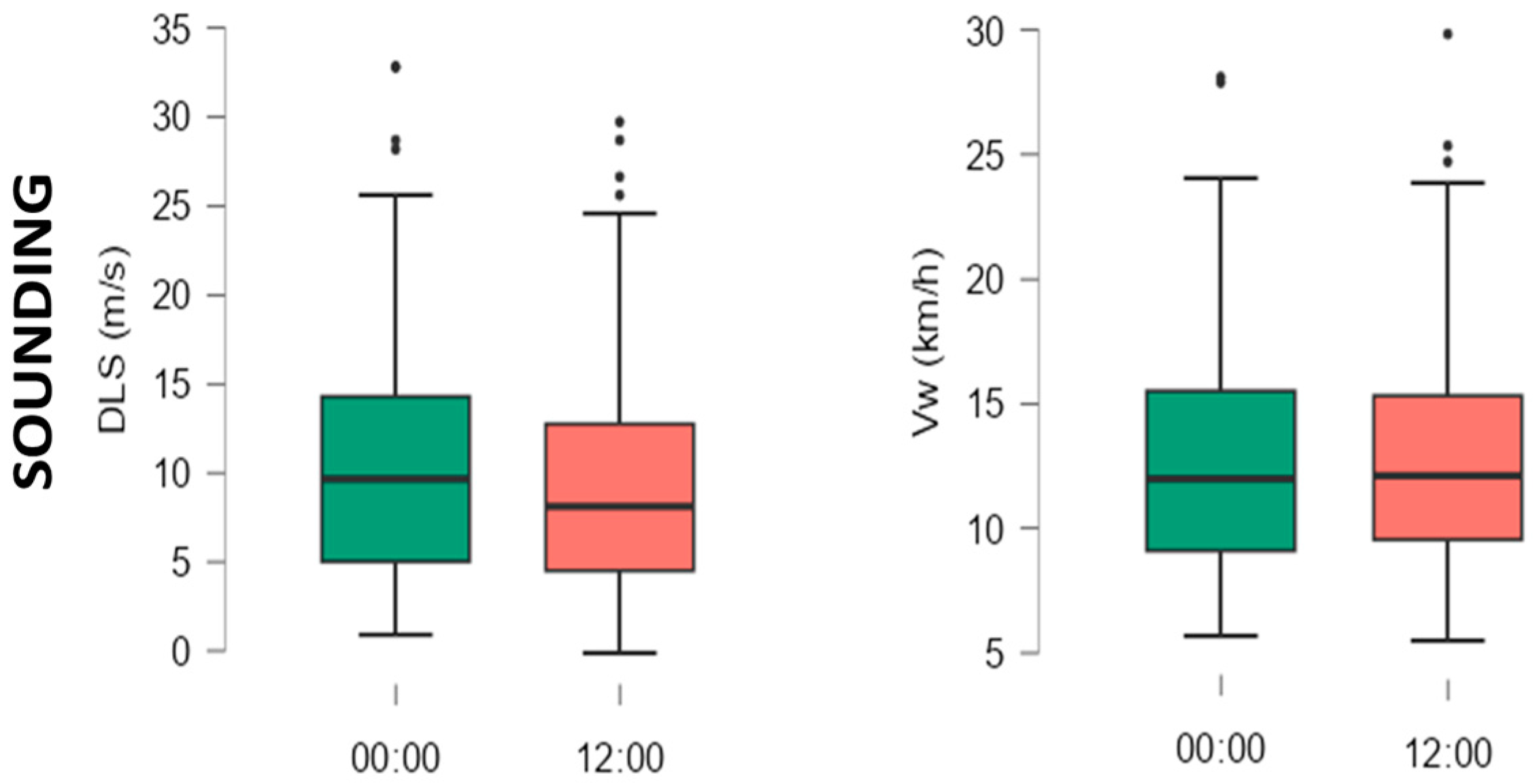
For all analysed hail cases, the DLS mean value is around 10 m/s for sounding data from 00 UTC and 8 m/s for those from 12 UTC (
Figure 5). The similar values are found in Central and Western Europe [
14,
24] and are greater (around 15 m/s) for hailstorms in the USA [
18,
26]. DLS upper quartile values exceed 10 m/s and reach a maximum of 20 m/s. Vw has values between 7 and 19 km/h, being a very useful index for determining the movement of convective clouds. Its values can be correlated with the speeds of air masses that cause atmospheric instability in the studied territory or with relief and microclimate conditions in the case of local convections.
3.1.5. Composite Parameters
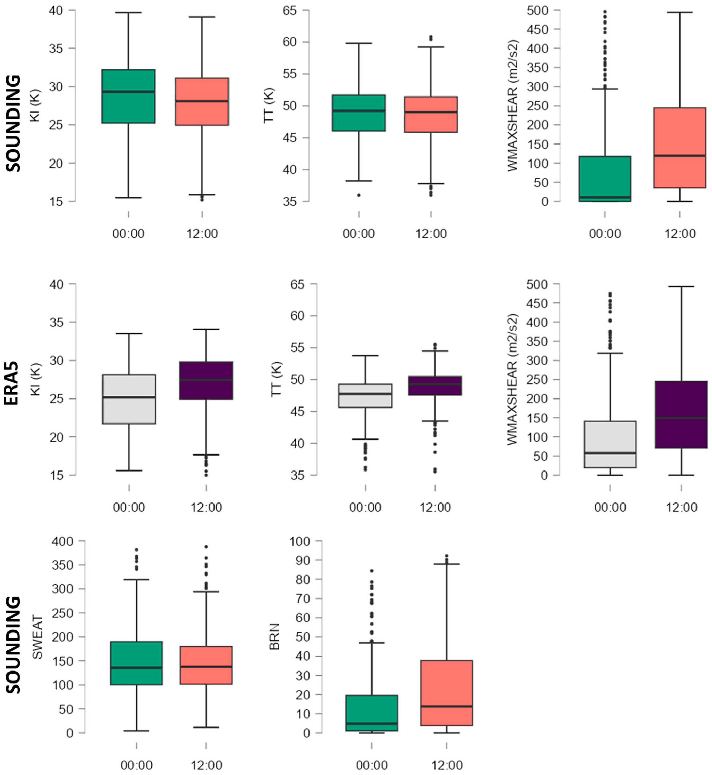
The TT and KI values indicate a moderately unstable environment with the probability of producing strong convective storms in limited areas (
Figure 6). The values of these two indices calculated from ERA5 are lower than those calculated from sounding data. KI does not stand out with values higher than 40. Values above 50 in the upper quartile of TT can highlight situations in the first part of the warm season when the instability was caused by cold air cores located at altitude (at the level of 500 hPa). WMAXSHEAR is a composite index that has shown a good potential to forecast strong atmospheric instability but also to differentiate the degree of the severity of convective phenomena [
14,
24]. The distribution of WMAXSHEAR values is closely related to that of CAPE, from which the updraft velocity is estimated. It is noted that the parameter values calculated from ERA5 are higher than those from the sounding data. For 00 UTC and only in 25% of cases, WMAXSHEAR indicates the possibility of some convection. Much more suggestive is the data from 12 UTC (from both data sources), which has a mean value of 150 m
2/s
2. These values are characteristic for the convective environment in more than 50% of the cases analysed.
Other two composite indices calculated from air sounding data, namely SWEAT and BRN, have values that indicate the existence of a convective environment favourable to the development of potential hail only for a part of the cases analysed in the study. In the case of SWEAT, the upper quartile values are between 150 and 300 (
Figure 6). These values indicate a reduced probability of the occurrence of strong storms, but it must be considered that the parameters of moisture from the low levels of the atmosphere and the parameters of instability, but also data related to the direction and speed of the vertical wind, are used in its calculation. Values in the lower quartile indicate an environment favourable to strong convection. The upper quartile includes values over 45 that characterise a weak and unstable environment.
3.2. Correlations among Parameters
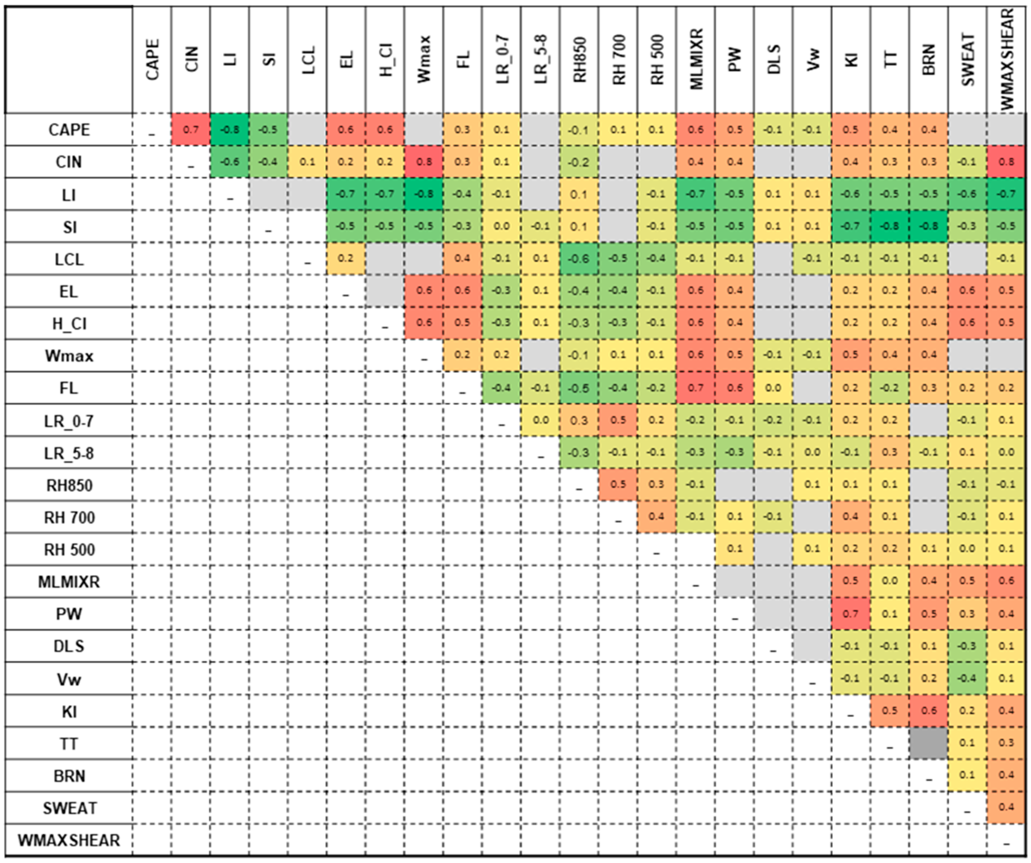
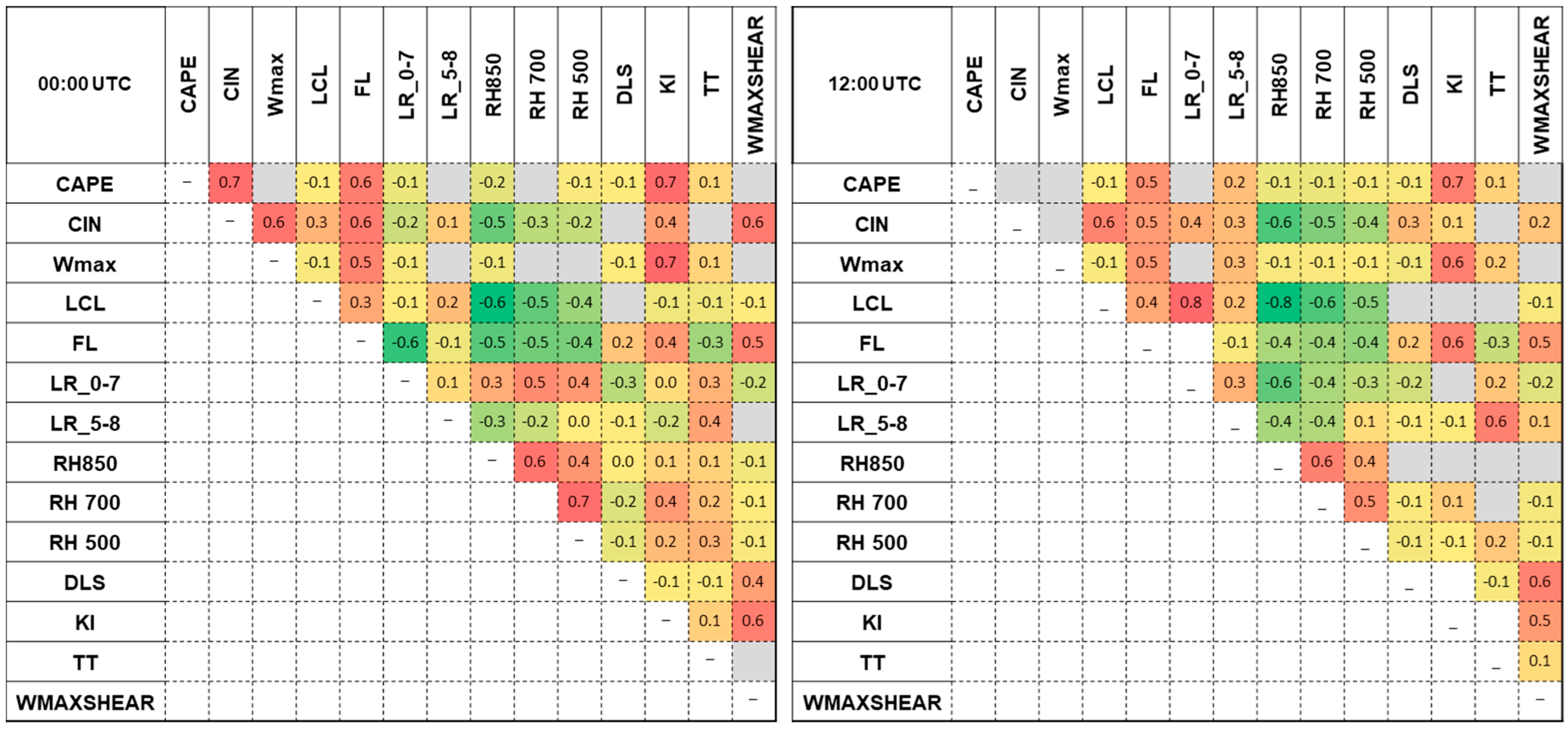
Derivative indices from a correlation matrix from sounding data at 00:00 UTC reveal very strong correlations between indices of the same type or from different “families” (
Figure 7). Coefficient values of 0.9 or higher are actually autocorrelations occurring between indices that are calculated with the same thermodynamic variables. In this situation, there are correlations between CAPE–BRN, LI–SI, KI–TT, or PW–MLMIXR. Other autocorrelations are recorded between CAPE and indices calculated using its value: Wmax; WMAXSHEAR. Good correlations were considered those with values of a Spearman correlation coefficient (rs) greater than 0.5. The correlation matrix shows two concentrations with integer coefficient values over 0.5. The most obvious are the high correlations between the indices calculated based on the particle theory. We found a strong correlation between indices calculated based on the particle theory and the moisture parameters, respectively, with the composite parameters. Correlations with coefficient values close to 0.5 also appear between the MLMIXR and the composite indices.
Strong negative correlations are recorded between LI, SI, and the other indicators due to the negative characteristic values of these two parameters. Other negative correlations such as those between EL and RH850 or FL and RH850 can be explained in terms of thermodynamic laws governing energy exchange in the lower and middle troposphere.
The correlation matrix between the parameters calculated from sounding data at 12:00 UTC (
Figure 8) shows the same pattern of rs coefficient values. The major difference lies in the higher correlation coefficient values between the particle theory-derived and moisture indices compared to the 00:00 UTC data. The index values at this time are the significant ones that characterise the convective environment, being the closest to the interval in which most of the hail events occurred.
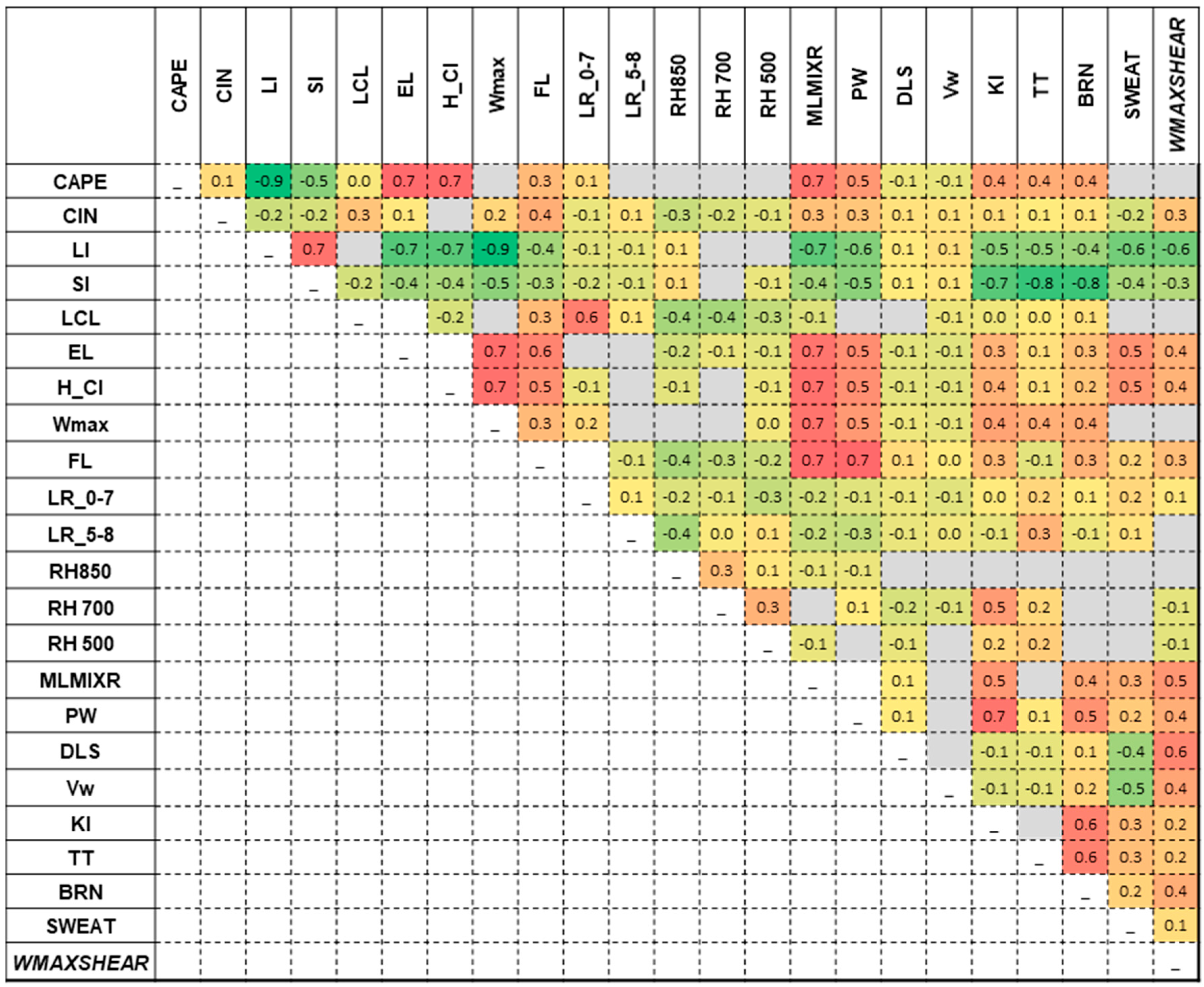
Correlation matrices for ERA5 parameters stand out as significant correlations between the same types of thermo-dynamic parameters as indices derived from air sounding (
Figure 9). Between CAPE and CIN exists a strong correlation only at 00:00 UTC observations. The correlation between night time CIN and CAPE and their lack at midday indicate that daytime heating and dynamical factors can convert convective inhibition into available energy for the development of convective hailstorms. In the case of the EL and LR_0-7 indices, a positive correlation present only from 12:00 UTC may be caused by cases where there is a reduced amount of moisture in the early troposphere. This situation involves the increase in the thermal gradient and implicitly of the air saturation deficit, which in turn causes the EL to increase.
Other good correlations are recorded between the relative humidity values at the three pressure levels, 850 hPa, 700 hPa, and 500 hPa, respectively. These indicate the presence of moist air layers in the lower and middle tropospheres.
4. Discussions
The highest values of the linear correlation coefficient (rs) were summarised in
Table 2 according to the groups in which the instability indices were classified. Correlations within the particle theory indices are recorded between LI or CAPE (Wmax) and the other indices. The decreased LI value and the increased CAPE value correlate very well with the H_Cl increase, indicating that the unstable layer can rise to very high altitudes in the troposphere in the presence of a strong vertical flow. A strong correlation exists between LI and CAPE. The LI negative value indicates that the planetary boundary layer is unstable in relation to the middle troposphere, and the high value of CAPE indicates a large amount of latent energy released following the condensation of water vapour. Generally, LI values lower than−4 correspond to CAPE values above 1000 J/kg. Atmospheric instability conditions are strongly influenced by synoptic patterns in the region. A recent study [
42] using the same hail data found the highest MUCAPE characterising the north–easterly anticyclonic flow. There are numerous situations where LI values indicate a moderate instability but CAPE indicates a low stability, which can be attributed to the existence of temperature inversions or an inhibitory layer. Istrate et al. [
37] obtained similar results for 140 hail days recorded in Romania between 2007 and 2018. The first category of indices also correlates very well with the amount of moisture in the lower troposphere, expressed by MLMIXRA as a larger amount of available water in the lower and middle tropospheres to be ascended at negative temperatures in the hail growth zone, indicated by the CAPE–MLMIXR, LI—MLMIXR, LI—PW, or Wmax–MLMIXR correlations.
Among the temperature indices, FL has the best correlations with EL and H_Cl. The increase in FL is associated with a stronger heating of the first part of the troposphere, which causes the increase in EL and H_Cl under conditions of instability.
Indices that capture the single-level instability of the atmosphere, LI and SI, are well correlated with KI, TT, and SWEAT values. However, they indicate stronger correlations between SI and the three indices mentioned. Those between SI-KI and SI-TT indicate that there is a thick layer of warm, moist air in the lower to middle troposphere, and a layer of cold air aloft. One of the correlations that can help to improve the forecast of hail is between the SI and SWEAT indexes. SI indicates the increase in the convective potential in the case of the approach of cold air masses that descend below the level of 850 mb. SWEAT takes into account several important parameters such as moisture in the lower troposphere, instability, and wind shear. Under the conditions of a cold atmospheric front, the accretion of hail is faster when the updraft contains a large amount of liquid water. The large amount of liquid water is determined by the high values of relative humidity in the lower troposphere.
High coefficient value correlations are found between FL and moisture parameters, such as MLMXR, RH850, and PW. In the summer months when the lower troposphere is warmer and richer in moisture, strong positive correlations could be found between FL–MLMXR and FL–PW. The negative coefficient between FL and RH850 can be explained by the influence that moisture in the lower troposphere, at 1500 m, (approximate altitude at which the 850 hPa level is usually found) has on the vertical thermal gradient.
An important limitation of our approach is the potential unrepresentativeness of the sounding data. Sounding stations are located hundreds of kilometres apart and data are collected only every 12 h, so that a relaxed criterion for proximity measurement was chosen in order to extract parameter data for all hail reports used. In addition, there are seasonal differences in parameter values, which must be discussed. For the future, we plan to use several parameters from ERA5, analyse them on a monthly basis, and establish a minimum forecast threshold, like the 25th percentile used by the authors of [
56].
5. Conclusions
Based on the multi-source hail reports’ data, as well as the sounding data and ERA5 reanalysis data in Northeastern Romania from 1981 to 2020, this paper statistically analyses the climatic characteristics of some convective parameters. The convective environment of hailstorms was studied using 23 instability parameters divided into five categories, namely particle theory indices, moisture indices, temperature indices, kinematic indices, and complex indices.
A statistical analysis of the instability parameters used indicates a significant difference in their values between 00:00 UTC and 12:00 UTC. The values of the indices at 12:00 UTC are much higher, some of them characterising the convective environment very well. The most used parameter, CAPE, has average values, at 12:00 UTC around 430 J/kg in the case of data from ERA5, and 505 J/kg in the case of data from sounding data, respectively. The average values at 00:00 UTC of this index are much lower, being below 200 J/kg, and in about 50% of the cases, they were very close or equal to 0. Moreover, forecasts of convective hazards are more difficult in situations of modest CAPE (<1000 J/kg) than large CAPE (>1000 J/kg).
The verification of the existence of some statistical correlations between the analysed indices was carried out using the Spearman correlation coefficient. Using correlation matrix of the derived indices from sounding data at the 00 UTC and 12 UTC, are distinguished very strong correlations between some indices. Good correlations were considered those with rs values greater than 0.5. The most obvious are the high correlations between the indices calculated based on the particle theory. Other strong correlations are those between particle theory parameters and the moisture parameters. The main conclusion is that the probability for large hail maximises with high values of low-level and boundary-layer moisture, high CAPE, and a high LCL height. We cannot, however, specify exactly which of the convective parameters are the most useful in hail forecasting. Following this analysis as well as the research in the field, it turns out that certain parameters are more important depending on the synoptic and local conditions. We consider it necessary to continue the research for the studied area and establish some minimum threshold values to be used in the operation of hail forecast.
Author Contributions
Conceptualisation, V.I. and D.P.; methodology, V.I. and D.A.S.; software, V.I., D.A.S. and E.P.; validation, E.S. and D.D.P.; data curation, V.I.; writing—original draft preparation, V.I. and D.P.; writing—review and editing, V.I. and D.P.; visualisation, E.S. and D.D.P. All authors have read and agreed to the published version of the manuscript.
Funding
This research received no external funding.
Data Availability Statement
ERA5 datasets used in this study are openly available and were downloaded from the European Centre for Medium-Range Weather Forecasts (ECMWF), Copernicus Climate Change Service (C3S) available at
https://cds.climate.copernicus.eu/. Sounding data were downloaded from the web server of the University of Wyoming.
Conflicts of Interest
The authors declare no conflict of interest.
References
- Hoeppe, P. Trends in weather related disasters—Consequences for insurers and society. Weather Clim. Extrem. 2016, 11, 70–79. [Google Scholar] [CrossRef]
- Fawbush, E.J.; Miller, R.C. A method for forecasting hailstone size at the earth’s surface. Bull. Am. Meteorol. Soc. 1953, 34, 235–244. Available online: https://www.jstor.org/stable/26242128 (accessed on 12 January 2023). [CrossRef]
- Foster, D.S.; Bates, F.C. A hail size forecasting technique. Bull. Am. Meteorol. Soc. 1956, 37, 135–141. [Google Scholar] [CrossRef]
- Miller, R.C. Notes on Analysis and Severe-Storm Forecasting Procedures of the Air Force Global Weather Central; Technical Report No 200; Headquarters, Air Weather Service, USAF: Bellevue, NE, USA, 1972; Available online: https://apps.dtic.mil/dtic/tr/fulltext/u2/744042.pdf (accessed on 12 January 2023).
- Renick, J.H.; Maxwell, J.B. Forecasting Hailfall in Alberta. In Hail: A Review of Hail Science and Hail Suppression; Foote, G.B., Knight, C., Eds.; American Meteorological Society: Boston, MA, USA, 1977; Volume 16, pp. 145–154. [Google Scholar] [CrossRef]
- Moore, J.T.; Pino, J.P. An interactive method for estimating maximum hailstone size from forecast soundings. Weather Forecast. 1990, 5, 508–525. [Google Scholar] [CrossRef]
- Doswell, C. Thermodynamic analysis procedures at the national severe storms forecast center. In Proceedings of the Conference on Weather Forecasting and Analysis, Seattle, WA, USA, 27 June–1 July 1982. [Google Scholar]
- Manzato, A. The use of sounding-derived indices for a neural network short-term thunderstorm forecast. Weather Forecast. 2005, 20, 896–917. [Google Scholar] [CrossRef]
- Groenemeijer, P.H.; van Delden, A. Sounding-derived parameters associated with large hail and tornadoes in the Netherlands. Atmos. Res. 2007, 83, 473–487. [Google Scholar] [CrossRef]
- Kunz, M. The skill of convective parameters and indices to predict isolated and severe thunderstorms. Nat. Hazards Earth Sys. Sci. 2007, 7, 327–342. [Google Scholar] [CrossRef]
- Sanchez, L.; Gil-Robles, B.; Dessens, J.; Martin, E.; López, L.; Marcos, J.; Berthe, C.; Fernández, J.T.; García-Ortega, E. Characterization of hailstone size spectra in hailpad networks in France, Spain, and Argentina. Atmos. Res. 2009, 93, 641–654. [Google Scholar] [CrossRef]
- Johnson, A.W.; Sugden, K.E. Evaluation of sounding-derived thermodynamic and wind-related parameters associated with large hail events. Electron. J. Severe Storms Meteorol. 2014, 9, 1–42. Available online: https://www.ejssm.org/ojs/idex.php/ejssm/article/view/137/101 (accessed on 13 January 2023). [CrossRef]
- Merino, A.; Wu, X.; Gascón, E.; Berthet, C.; García-Ortega, E.; Dessens, J. Hailstorms in southwestern France: Incidence and atmospheric characterization. Atmos. Res. 2014, 140, 61–75. [Google Scholar] [CrossRef]
- Púčik, T.; Groenemeijer, P.; Rýv, D.; Kolář, M. Proximity Soundings of Severe and Nonsevere Thunderstorms in Central Europe. Mon. Weather Rev. 2015, 143, 4805–4821. Available online: https://journals.ametsoc.org/view/journals/mwre/143/12/mwr-d-15-0104.1.xml (accessed on 13 January 2023). [CrossRef]
- Tuovinen, J.P.; Rauhala, J.; Schultz, D.M. Significant-hail-producing storms in Finland: Convective-storm environment and mode. Weather Forecast. 2015, 30, 1064–1076. [Google Scholar] [CrossRef]
- Lkhamjav, J.; Jin, H.-G.; Lee, H.; Baik, J.-J. A hail climatology in Mongolia. Asia-Pac. J. Atmos. Sci. 2017, 53, 501–509. [Google Scholar] [CrossRef]
- Lin, Y.; Kumjian, M.R. Influences of CAPE on Hail Production in Simulated Supercell Storms. J. Atmos. Sci. 2022, 79, 179–204. [Google Scholar] [CrossRef]
- Craven, J.P.; Brooks, H.E. Baseline climatology of sounding derived parameters associated with deep moist convection. Natl. Weather Dig. 2004, 28, 13–24. [Google Scholar]
- Abshaev, M.T.; Goral, G.G.; Malbakhova, N.M. Hail type forecast. Geophys. Inst. Nalicic 1965, 67, 72–79. [Google Scholar]
- Fedchenko, L.M.; Belentsova, V.A.; Berova, M.A. Forecast of intensive hail processes in the North Caucasus. Geophys. Inst. Nalicic 1981, 50, 21–35. [Google Scholar]
- Goral, G.G.; Barekova, M.V. Potential atmospheric instability and hail forecast in Armenia. Geophys. Inst. Nalicic 1986, 63, 48–57. [Google Scholar]
- Fedchenko, G.L.M.; Goral, G.G.; Malbakhova, N.M. Detailed methods of hail forecast. Atmos. Res. 1992, 28, 375–384. [Google Scholar] [CrossRef]
- Weisman, M.L.; Klemp, J.B. The dependence of numerically simulated convective storms on vertical wind shear and buoyancy. Mon. Weather Rev. 1982, 110, 504–520. [Google Scholar] [CrossRef]
- Taszarek, M.; Brooks, H.E.; Czernecki, B. Sounding-Derived Parameters Associated with Convective Hazards in Europe. Mon. Weather Rev. 2017, 145, 1511–1528. [Google Scholar] [CrossRef]
- Taszarek, M.; Allen, J.T.; Groenemeijer, P.; Edwards, R.; Brooks, H.E.; Chmielewsk, V.; Enno, S. Severe convective storms across Europe and the United States. Part 1: Climatology of lightning, large hail, severe wind and tornadoes. J. Clim. 2020, 33, 10239–10261. [Google Scholar] [CrossRef]
- Taszarek, M.; Allen, J.T.; Púčik, T.; Hoogewind, K.A.; Brooks, H.E. Severe Convective Storms across Europe and the United States. Part II: ERA5 Environments Associated with Lightning, Large Hail, Severe Wind, and Tornadoes. J. Clim. 2020, 33, 10263–10286. [Google Scholar] [CrossRef]
- Kunz, M.; Wandel, J.; Fluck, E.; Baumstark, S.; Mohr, S.; Schemm, S. Ambient conditions prevailing during hail events in central Europe. Nat. Hazards Earth Syst. Sci. 2020, 20, 1867–1887. [Google Scholar] [CrossRef]
- Edwards, R.; Thompson, R.L. Nationwide comparisons of hail size with WSR-88D vertically integrated liquid water and derived thermodynamics sounding data. Weather Forecast. 1998, 13, 277–285. [Google Scholar] [CrossRef]
- Allen, J.T.; Tippett, M.K.; Sobel, A.H. An empirical model relating U.S. monthly hail occurrence to large-scale meteorological environment. J. Adv. Model. Earth Syst. 2015, 7, 226–243. [Google Scholar] [CrossRef]
- McCaul, J.; Cohen, C. The impact on simulated storm structure and intensity of variations in the mixed layer and moist layer depths. Mon. Weather Rev. 2022, 130, 1722–1748. [Google Scholar] [CrossRef]
- Bălescu, O.I.; Militaru, F. Aerological study of hail falls. Collect. Pap. Meteorol. Inst. 1967, 24, 73–85. [Google Scholar]
- Grama, M. Methods for forecasting Cumulonimbus clouds and thunderstorms at Bucharest-Băneasa airport. Collect. Pap. Meteorol. Inst. 1969, 26, 153–160. [Google Scholar]
- Ionescu-Nișcov, Ș. Forecast of stormy phenomena within the mass applying some of the methods of mathematical statistics. Stud. Res. Part I Meteorol. 1978, 23, 283–294. [Google Scholar]
- Sfîcă, L.; Apostol, L.; Istrate, V.; Lesenciuc, D.; Necula, M.F. Instability indices as predictors of atmospheric lightning—Moldova region study case. In Proceedings of the SGEM 2015, Albena, Bulgaria, 18–24 June 2015; pp. 387–394. [Google Scholar] [CrossRef]
- Istrate, V.; Axinte, A.D.; Florea, D.; Bărcăcianu, F.; Apostol, L. Characteristics and impacts of the severe hailstorms on 18 June 2016 in northern Moldavia, Romania. In Proceedings of the 19th International SGEM 2019, Albena, Bulgaria, 28 June–7 July 2019; Volume 19, pp. 899–906. [Google Scholar] [CrossRef]
- Ilie, N.; Apostol, L.; Axinte, A.D. The way to determine the approximately hail’s dimensions. Present Environ. Sustain. Dev. 2020, 14, 209–219. [Google Scholar] [CrossRef]
- Istrate, V.; Dobri, R.V.; Bărcăcianu, F.; Ciobanu, R.A.; Apostol, L. Sounding-derived parameters associated with severe hail events in Romania. Időjárás 2021, 125, 39–52. [Google Scholar] [CrossRef]
- Istrate, V.; Jitariu, V.; Ichim, P.; Machidon, O.M.; Apostol, L. Hailstorm risk assessment for crop areas in Moldova Region (Romania). Present Environ. Sustain. Dev. 2021, 15, 55–67. [Google Scholar] [CrossRef]
- Burcea, S.; Cică, R.; Bojariu, R. Hail Climatology and Trends in Romania: 1961–2014. Mon. Weather Rev. 2016, 144, 4289–4299. [Google Scholar] [CrossRef]
- Rusu, A.; Ursu, A.; Stoleriu, C.C.; Groza, O.; Niacșu, L.; Sfîcă, L.; Minea, I.; Stoleriu, O.M. Structural Changes in the Romanian Economy Reflected through Corine Land Cover Datasets. Remote Sens. 2020, 12, 1323. [Google Scholar] [CrossRef]
- Apostol, L.; Sfîcă, L. Thermal differentiations induced by the Carpathian Mountains on the Romanian territory. Carpath. J. Earth Environ. Sci. 2013, 8, 215–221. [Google Scholar]
- Sfîcă, L.; Istrate, V.; Hrițac, R.; Machidon, O. The continental and regional synoptic background favorable for hailstorms occurrence in North-Eastern Romania. Prog. Phys. Geogr. Earth Environ. 2023, 47, 3–31. [Google Scholar] [CrossRef]
- Púčik, T.; Castellano, C.; Groenemeijer, P.; Kühne, T.; Rädler Anja, T.; Antonescu, B.; Faust, E. Large hail incidence and its economic and societal impacts across Europe. Mon. Weather Rev. 2019, 147, 3901–3916. [Google Scholar] [CrossRef]
- Dotzek, N.; Forster, C. Quantitative comparison of METEOSAT thunderstorm detection and nowcasting with in situ reports in the European Severe Weather Database (ESWD). Atmos. Res. 2011, 100, 511–522. [Google Scholar] [CrossRef]
- Istrate, V.; Dobri, R.V.; Bărcăcianu, F.; Ciobanu, R.A.; Apostol, L. A ten years hail climatology based on ESWD hail reports in Romania, 2007–2016. Geogr. Tech. 2017, 12, 110–118. [Google Scholar] [CrossRef]
- Añel, J.A.; Sáenz, G.; Ramírez-González, I.A.; Polychroniadou, E.; Vidal-Mina, R.; Gimeno, L.; de la Torre, L. Obtaining meteorological data from historical newspapers: La Integridad. Weather 2017, 72, 366–371. [Google Scholar] [CrossRef]
- Cheval, S.; Haliuc, A.; Antonescu, B.; Tișcovschi, A.; Dobre, M.; Tătui, F.; Dumitrescu, A.; Manea, A.; Tudorache, G.; Irimescu, A.; et al. Enriching the historical meteorological information using Romanian language newspaper reports: A database from 1880 to 1900. Int. J. Climatol. 2021, 41, E548–E562. [Google Scholar] [CrossRef]
- University of Wyoming Sounding Data. Available online: http://www.weather.uwyo.edu/upperair/sounding.html (accessed on 20 September 2020).
- Cohen, A.E.; Coniglio, M.C.; Corfidi, S.F.; Corfidi, S.J. Discrimination of mesoscale convective system environments using sounding observations. Weather Forecast. 2007, 22, 1045–1062. [Google Scholar] [CrossRef]
- Hersbach, H.; Bell, B.; Berrisford, P.; Hirahara, S.; Horányi, A.; Muñoz-Sabater, J.; Nicolas, J.; Peubey, C.; Radu, R.; Schepers, D.; et al. The ERA5 global reanalysis. Q. J. R. Meteorol. Soc. 2020, 146, 1999–2049. [Google Scholar] [CrossRef]
- Palencia, C.; Giaiotti, D.; Stel, F.; Castro, A.; Fraile, R. Maximum hailstone size: Relationship with meteorological variables. Atmos. Res. 2010, 96, 256–265. [Google Scholar] [CrossRef]
- Kunz, M.; Sander, J.; Kottmeier, C. Recent trends of thunderstorm and hailstorm frequency and their relation to atmospheric characteristics in southwest Germany. Int. J. Climatol. 2009, 29, 2283–2297. [Google Scholar] [CrossRef]
- Manzato, A. Hail in Northeast Italy: Climatology and bivariate analysis with the sounding-derived indices. J. Appl. Meteorol. Climatol. 2012, 51, 449–467. [Google Scholar] [CrossRef]
- Dessens, J.; Berthet, C.; Sanchez, J.L. Change in hailstone size distributions with an increase in the melting level height. Atmos. Res. 2015, 158–159, 245–253. [Google Scholar] [CrossRef]
- Kaltenböck, R.; Diendorfer, G.; Dotzek, N. Evaluation of thunderstorm indices from ECMWF analyses, lightning data and severe storm reports. Atmos. Res. 2009, 93, 381–396. [Google Scholar] [CrossRef]
- Tang, J.; Xu, L.; Yao, R.; Ou, X.; Long, Q.; Wang, X. Characteristics of Environmental Parameters of Compound and Single Type Severe Convection in Hunan. Atmosphere 2022, 13, 1870. [Google Scholar] [CrossRef]
Figure 1.
Geographical position of northeastern Romania and at a country scale (a); spatial distribution of the mean annual hail frequency (residual kriging interpolation based on data from 18 meteorological stations) (b), monthly distribution of the hail events (c), and hourly distributions of the hail events (d) for 1981–2020.
Figure 2.
Box-and-whisker plots for parcel theory parameters. The median is represented as a horizontal line inside the box, the edges of the box represent the 25th and 75th percentiles, while whiskers represent the 10th and 90th percentiles.
Figure 2.
Box-and-whisker plots for parcel theory parameters. The median is represented as a horizontal line inside the box, the edges of the box represent the 25th and 75th percentiles, while whiskers represent the 10th and 90th percentiles.
Figure 3.
Box-and-whisker plots for temperature parameters. The median is represented as a horizontal line inside the box, the edges of the box represent the 25th and 75th percentiles, while whiskers represent the 10th and 90th percentiles.
Figure 3.
Box-and-whisker plots for temperature parameters. The median is represented as a horizontal line inside the box, the edges of the box represent the 25th and 75th percentiles, while whiskers represent the 10th and 90th percentiles.
Figure 4.
Box-and-whisker plots for moisture parameters. The median is represented as a horizontal line inside the box, the edges of the box represent the 25th and 75th percentiles, while whiskers represent the 10th and 90th percentiles.
Figure 4.
Box-and-whisker plots for moisture parameters. The median is represented as a horizontal line inside the box, the edges of the box represent the 25th and 75th percentiles, while whiskers represent the 10th and 90th percentiles.
Figure 5.
Box-and-whisker plots for kinematic parameters. The median is represented as a horizontal line inside the box, the edges of the box represent the 25th and 75th percentiles, while whiskers represent the 10th and 90th percentiles.
Figure 5.
Box-and-whisker plots for kinematic parameters. The median is represented as a horizontal line inside the box, the edges of the box represent the 25th and 75th percentiles, while whiskers represent the 10th and 90th percentiles.
Figure 6.
Box-and-whisker plots for composites parameters. The median is represented as a horizontal line inside the box, the edges of the box represent the 25th and 75th percentiles, while whiskers represent the 10th and 90th percentiles.
Figure 6.
Box-and-whisker plots for composites parameters. The median is represented as a horizontal line inside the box, the edges of the box represent the 25th and 75th percentiles, while whiskers represent the 10th and 90th percentiles.
Figure 7.
Correlation matrix for 23 instability indices derived from sounding data at 00:00 UTC. Spearman correlation coefficient (rs) values indicating strong correlations are marked with the darkest shades of red and green (warm colours represent positive rs values and cold colours negative values). Significance level α = 0.05. Autocorrelations and insignificant correlations less than ‖0.1‖ are marked in grey.
Figure 8.
Correlation matrix for 23 instability indices derived from sounding data at 12:00 UTC. Spearman correlation coefficient (rs) values indicating strong correlations are marked with the darkest shades of red and green (warm colours represent positive rs values and cold colours negative values). Significance level α = 0.05. Autocorrelations and insignificant correlations less than ‖0.1‖ are marked in grey.
Figure 9.
Correlation matrix for 14 mean instability indices values derived from ERA5 data at 00:00 UTC and 12:00 UTC. Spearman correlation coefficient (rs) values indicating strong correlations are marked with the darkest shades of red and green (warm colours represent positive rs values and cold colours negative values).Significance level α = 0.05. Autocorrelations and insignificant correlations smaller than ‖0.1‖ are marked in grey.
Table 1.
Parameters used in study.
Table 1.
Parameters used in study.
| | Group | Index Name | Acronym | Unit of Measure |
|---|
| 1 | Parcel parameters
(based on most
instable parcels) | Convective available potential energy | CAPE | J/kg |
| 2 | Convective inhibition | CIN | J/kg |
| 3 | Lifted Index | LI | - |
| 4 | Showalter index | SI | °C |
| 5 | Lifting condensation level | LCL | m |
| 6 | Equilibrium level | EL | m |
| 7 | Cloud vertical extent | H_Cl | m |
| 8 | Parcel’s max vertical velocity (square root of 2 × CAPE) | Wmax | m/s |
| 9 | Temperature
indices | Freezing level | FL | m |
| 10 | Lapse rate, 2 m–700 hPa | LR_0-7 | °C/km |
| 11 | Lapse rate, 800–500 hPa | LR_5-8 | °C/km |
| 12 | Moisture indices | Relative humidity at 850 hPa pressure level | RH850 | % |
| 13 | Relative humidity at 700 hPa pressure level | RH 700 | % |
| 14 | Relative humidity at 500 hPa pressure level | RH 500 | % |
| 15 | Mean mixed layer MIXR (average MIXR in the lowest 500 m) | MLMIXR | g/kg |
| 16 | Precipitable water | PW | mm |
| 17 | Kinematic indices | AGL wind shear–deep-layer shear, 0–6 km | DLS | m/s |
| 18 | Velocity of the mainstream | Vw | km/h |
| 19 | Composite indices | K index | KI | K |
| 20 | Total totals | TT | K |
| 21 | Bulk Richardson number | BRN | - |
| 22 | Severe weather threat index | SWEAT | - |
| 23 | DLS × Wmax | WMAXSHEAR | m2/s2 |
Table 2.
Strong linear correlations between index values derived from sounding data at 00:00 UTC and 12:00 UTC of the 378 hail days analysed.
Table 2.
Strong linear correlations between index values derived from sounding data at 00:00 UTC and 12:00 UTC of the 378 hail days analysed.
| Parameters | Couples | Spearman Corelation Coefficient (rs) |
|---|
| 00:00 UTC | 12:00 UTC |
|---|
| Between parcel parameters | CAPE–LI | −0.80 | −0.90 |
| | CAPE–H_Cl | 0.60 | 0.69 |
| LI–LCL | −0.70 | −0.70 |
| LI–H_Cl | −0.70 | −0.70 |
| LI–Wmax | −0.80 | −0.90 |
| LCL–LR_0-7 | 0.60 | 0.70 |
| LCL–Wmax | 0.60 | 0.70 |
| Between parcel parameters and moisture parameters | CAPE–MLMIXR | 0.60 | 0.70 |
| LI–MLMXR | −0.70 | −0.70 |
| EL–MLMIXR | 0.60 | 0.70 |
| H_Cl–MLMIXR | 0.60 | 0.70 |
| Wmax–MLMIXR | 0.60 | 0.70 |
| Wmax–PW | 0.50 | 0.50 |
| Between parcel parameters and temperature parameters | H_Cl–FL | 0.60 | 0.50 |
| Between parcel parameters and composite parameters | SI–KI | −0.70 | −0.70 |
| SI–TT | −0.80 | −0.80 |
| SI–SWEAT | −0.80 | −0.80 |
| Wmax–KI | 0.50 | 0.30 |
| Between temperature parameters and moisture parameters | FL–MLMIXR | 0.70 | 0.70 |
| FL–PW | 0.60 | 0.70 |
| Between composite parameters and moisture parameters | KI–PW | 0.70 | 0.70 |
| WMAXSHEAR–MLMIXR | 0.60 | 0.50 |
| Disclaimer/Publisher’s Note: The statements, opinions and data contained in all publications are solely those of the individual author(s) and contributor(s) and not of MDPI and/or the editor(s). MDPI and/or the editor(s) disclaim responsibility for any injury to people or property resulting from any ideas, methods, instructions or products referred to in the content. |
© 2023 by the authors. Licensee MDPI, Basel, Switzerland. This article is an open access article distributed under the terms and conditions of the Creative Commons Attribution (CC BY) license (https://creativecommons.org/licenses/by/4.0/).


