Influence of Underlying Topography on Post-Monsoon Cyclonic Systems over the Indian Peninsula

Abstract

During the post-monsoon cyclone season, the landfalls of westward-moving cyclonic systems often lead to extreme rainfall over the east coast of the Indian peninsula. A stationary cyclonic system over the coast can produce heavy rainfall for several days and cause catastrophic flooding. This study analyzes the dynamics of a propagating and stationary cyclonic system over the east coast, highlighting the possible cause behind the stagnation. The vorticity budgets of these two systems are presented using a reanalysis dataset. Vortex stretching and horizontal vorticity advection were the dominant terms in the budget. Vertical advection and tilting terms were significant over the orography. The horizontal advection of vorticity was positive (negative) on the western (eastern) side of the systems and, thus, favored westward propagation. Vortex stretching was confined to the upstream of orography in the stationary vortex. In the propagating vortex, the vortex stretching occurred over the orography during its passage. Data from the radiosonde soundings over a coastal station showed orographic blocking of the low-level winds in the stationary case. Conversely, the flow crossed the orographic barrier in the propagating case. Thus, the predominance of the upstream orographic convergence over the vortex circulation can be the reason for system stagnation over the coast.

1. Introduction

Tropical depressions and cyclones are among the leading causes of weather-related natural calamities. Convection over the Northern Indian Ocean is often organized in the form of tropical depressions. These are pre-hurricane weather systems wherein the large-scale flow can be assumed to be in a hydrostatic and gradient wind balance [1]. These cyclonic vortices, in the absence of a prevailing steering flow, have an inclination to move westward–northwestward due to the planetary $\beta$-effect [2,3,4,5]. During the post-monsoon cyclone season (October–December), these cyclonic systems predominantly form over the eastern equatorial Indian Ocean (85–95${}^{\circ }$ E and 0–10${}^{\circ }$ N). These systems subsequently move northwestward to make landfall over the densely populated Coromandel Coast over the Indian peninsula (Figure 1); some of them curve back northeastwards and make landfall over the Bangladesh–Myanmar coast. The northeastward propagation of cyclonic systems can be explained by the advection of vorticity by the upper-level jet [6]. During this time of the year, a 30–50 m deep warm layer of fresh water from river run-offs and summer monsoon rainfall sits over the northern part of the Bay of Bengal and fuels the growth of these vortices [7]. The tropical depressions are better organized (strengthened) with the time they spend over the warm ocean. A vortex of a Tropical Cyclone’s (TC) strength can cause widespread damage after landfall due to strong winds, storm surges, and heavy rainfall. Slow-moving/quasi-stationary systems can deposit a large amount of rainfall and cause severe flooding, e.g., Hurricane Harvey stalling over Texas, USA [8]. Loss of life and property due to stationary systems, even in the case of weaker ones, can be far more severe.

During the post-monsoon cyclone season of 2015, the arrival of back-to-back tropical depressions led to repeated flooding events over the Coromandel Coast [9]. During 30 November–2 December 2015, a stationary cyclonic circulation led to disastrous flooding in Chennai city [10]. At least 250 people died in the flood [11]. On 1 December, 494 mm rainfall was reported within 24 h. Phadtare [10] performed WRF simulations of the 1 December 2015 Chennai extreme rainfall event and showed that the orographic blocking of the evaporative cold pool led to coastal stagnation and organization of deep convection. The cyclonic system also remained stationary over the coast for 2–3 days and subsequently moved southwards. Boyaj et al. [12] attributed the increased intensity of rainfall events over the coast to the ongoing El-Niño conditions and the connected warming in the Bay of Bengal. While there are many previous studies suggesting a link between El-Niño and above normal rainfall over peninsular India during October–December [13,14,15,16,17,18], Krishnamurthy et al. [19] associated the extreme rainfall exclusively with the Bay of Bengal warming. They further suggested that the probability of extreme rainfall events over the coast is high in the presence of a tropical depression. The extreme rainfall intensity of 1 December 2015 has a return period of 600–2500 years over the Coromandel Coast [20]. This implies that the severity of the rainfall accumulation was much greater than a TC event. As far as TCs are concerned, the forecasting of their paths over the open oceans using numerical weather models has improved over the last couple of decades [21], including in the Indian Ocean region [22,23,24,25,26,27]. However, the phenomenon of post-landfall stagnation of cyclonic vortices has not received much attention. Therefore, our understanding of the dynamics of slow-moving cyclonic vortices and the conditions in which they become stagnated is poor. The analysis of the vorticity balance in the stagnated and moving cyclonic vortices can provide us with some clues on the dominant processes in the two cases.

The movement of a cyclonic vortex is determined by the time tendency of the vorticity field, which mainly depends on vorticity advection by the flow, vorticity increase by vortex stretching, and dissipation due to surface friction [28,29,30,31,32]. The cyclonic flow of the system leads to nonlinear advection of absolute (planetary plus relative) vorticity to the northwest of the initial vortex center [3]. Thus, the cyclonic vortex tends to move northwestwards if it is not steered by a strong background jet [6]. The latent heat release in precipitating clouds can also alter the vorticity field of these vortices by inducing ascent and convergence [1,33,34]. Charney and Ellassen [1] proposed that the latent heat released into the clouds provides the necessary energy for the growth of hurricanes by providing positive feedback to large-scale convergence. Stoelinga [34], using a mesoscale numerical model, showed that the latent heat due to the condensation alone contributes to about 70% of the surface cyclone strength. Using a quasi-geostrophic model, Raymond and Jiang [33], suggested that the latent heat released in clouds leads to low-level potential vorticity generation, which prolongs the life of a mesoscale convective system. Boos et al. [32] show that the latent heat associated with stratiform clouds affects the propagation of monsoonal depressions.

Zehnder [35] showed that the topography of Mexico can deflect the westward moving cyclonic vortices towards the south. Over the Indian peninsula, the Eastern Ghats mountain range (average height ≃ 750 m) lies parallel, and about 200 km inland, to the Coromandel Coast (Figure 1). The upstream orographic blocking of easterly winds by the Eastern Ghats mountains, and the subsequent stagnation of precipitating clouds and the cyclonic system was the reasons for the extreme rainfall event over Chennai on 1 December 2015 [10]. A similar event occurred over the coast during 15–18 November 2015, causing a severe flood in which about 70 people died [36].

In this study, post-landfall dynamics of two cyclonic vortices along the Coromandel Coast are analyzed. The first (henceforth, ‘Vortex-1’) crossed the Indian peninsula during 9–11 November 2015, while the second (henceforth, ‘Vortex-2’) was stationary over the coast during 15–18 November 2015. The propagation mechanisms of the two vortices were investigated through their vorticity budgets and a criterion for coastal vortex stagnation is proposed. Section 2 describes the datasets used in this study. Section 3 shows the evolution of Vortex-1 and Vortex-2 along with the convection and rainfall fields of these vortices. Section 4 explains the influence of topography on the vorticity structures of these vortices. Section 5 contains a summary and recommendations for further research.

2. Data

2.1. Dynamics

The fifth-generation European Center for Medium-Range Weather Forecasts (ECMWF) atmospheric reanalysis of the global climate (ERA5) [37] dataset is used for analyzing the dynamics of vortices. ERA5 has 31 km of spatial and hourly temporal resolution, and is available on 137 vertical levels until 0.01 hPa. Since the vortices slow down during the landfall, vorticity budgets are calculated with daily mean fields. Radiosonde-sounding data from Chennai were used to obtain the high-resolution wind and stratification profiles of the atmosphere along the coast. The high-resolution data from soundings are useful to determine the orographic blocking of the winds [10,38,39].

2.2. Convection and Rainfall

Infrared (IR∼10.8 $\mathsf{\mu }$m) images from the INSAT-3D satellite, located over ${82}^{\circ }$ E, are used to visualise the organization of deep convection within the vortices. The INSAT-3D IR images have 4 km spatial and 30-min of temporal resolution. These images are archived by the Meteorological and Oceanographic Satellite Data Archival Center (MOSDAC), Satellite Applications Center (SAC), Indian Space Research Organization (ISRO). The Final Run version (V06B) of the integrated multi-satellite retrievals for GPM (IMERG V06B) rainfall product [40] provided by the National Aeronautics and Space Administration (NASA) is used for rainfall. IMERG has 10 km of spatial and 30-min of temporal resolution.

3. Event Description

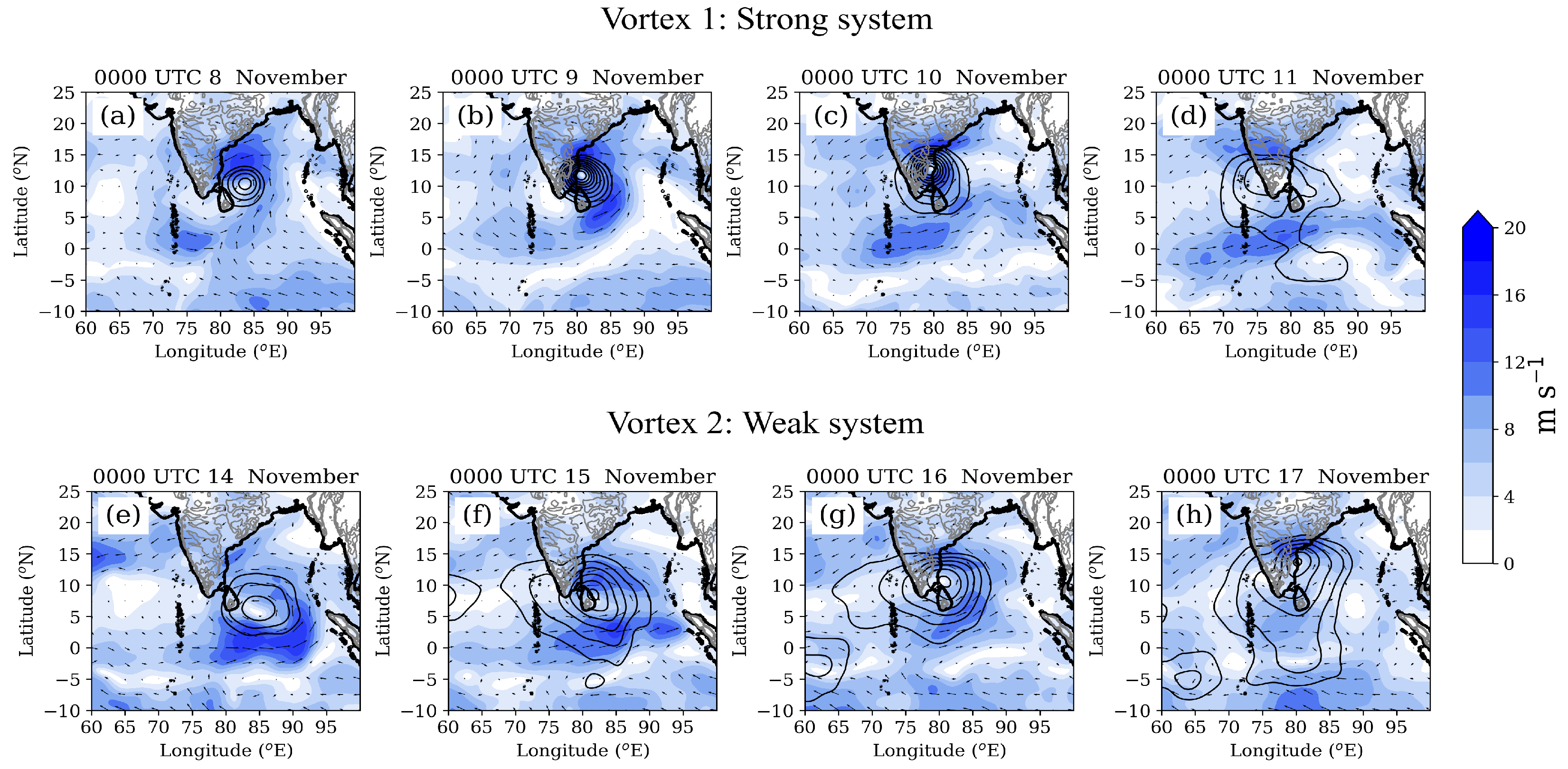
3.1. Propagation of Vortices

Figure 2 shows propagations of Vortex-1 and Vortex-2 over the Coromandel Coast. Vortex-1, with a maximum speed of about 20 m s${}^{-1}$, is stronger among the two vortices. It arrived over the coast on 9 November (Figure 2b). It moved inland thereafter; on 11 November, it moved over the orographic peaks (Figure 2d). Vortex-2, on the other hand, hovered over the coast for three days (15–17 November), and also became elongated (compressed) in the meridional (zonal) direction, i.e., it aligned itself with the underlying topography (Figure 2e–h). Both vortices are embedded in weak background flows, i.e., their external steering is weak.

Figure 3 shows the vertical cross-section of the daily mean relative vorticity ($\zeta$) and $\zeta$ tendency ($\partial \zeta$/$\partial t$) for Vortex-1 and Vortex-2. Vortex-1 (Figure 3a–d) moves from the east of the topography to its west in four days. Whereas, Vortex-2 remains anchored on the east coast. The upright structure of Vortex-2 (Figure 3e) also becomes tilted after landfall (Figure 3f–h). Note that the low-level vorticity contours of tilted Vortex-2 align parallel to the orographic slope.

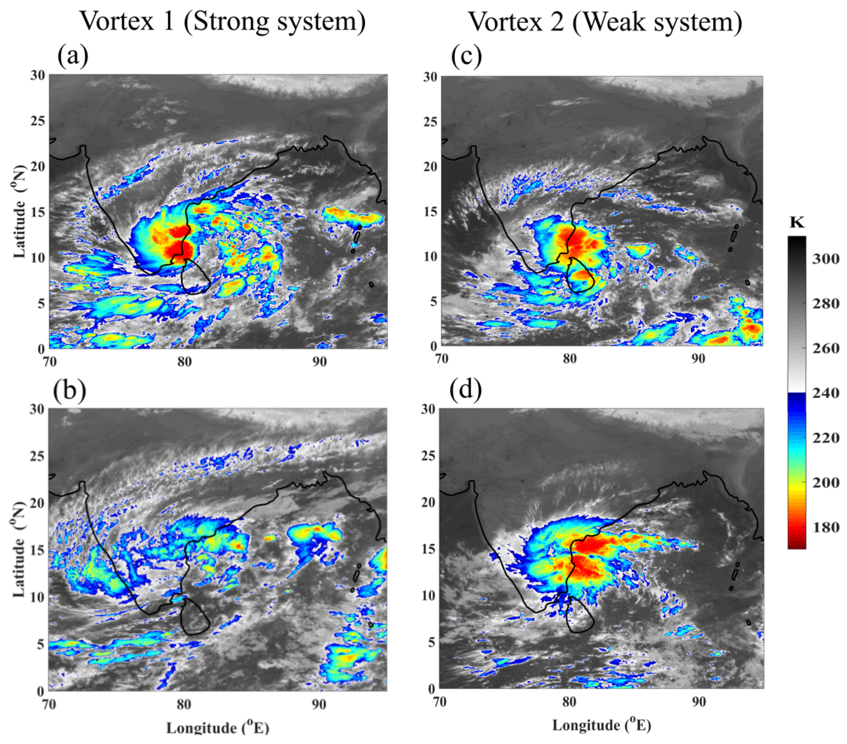
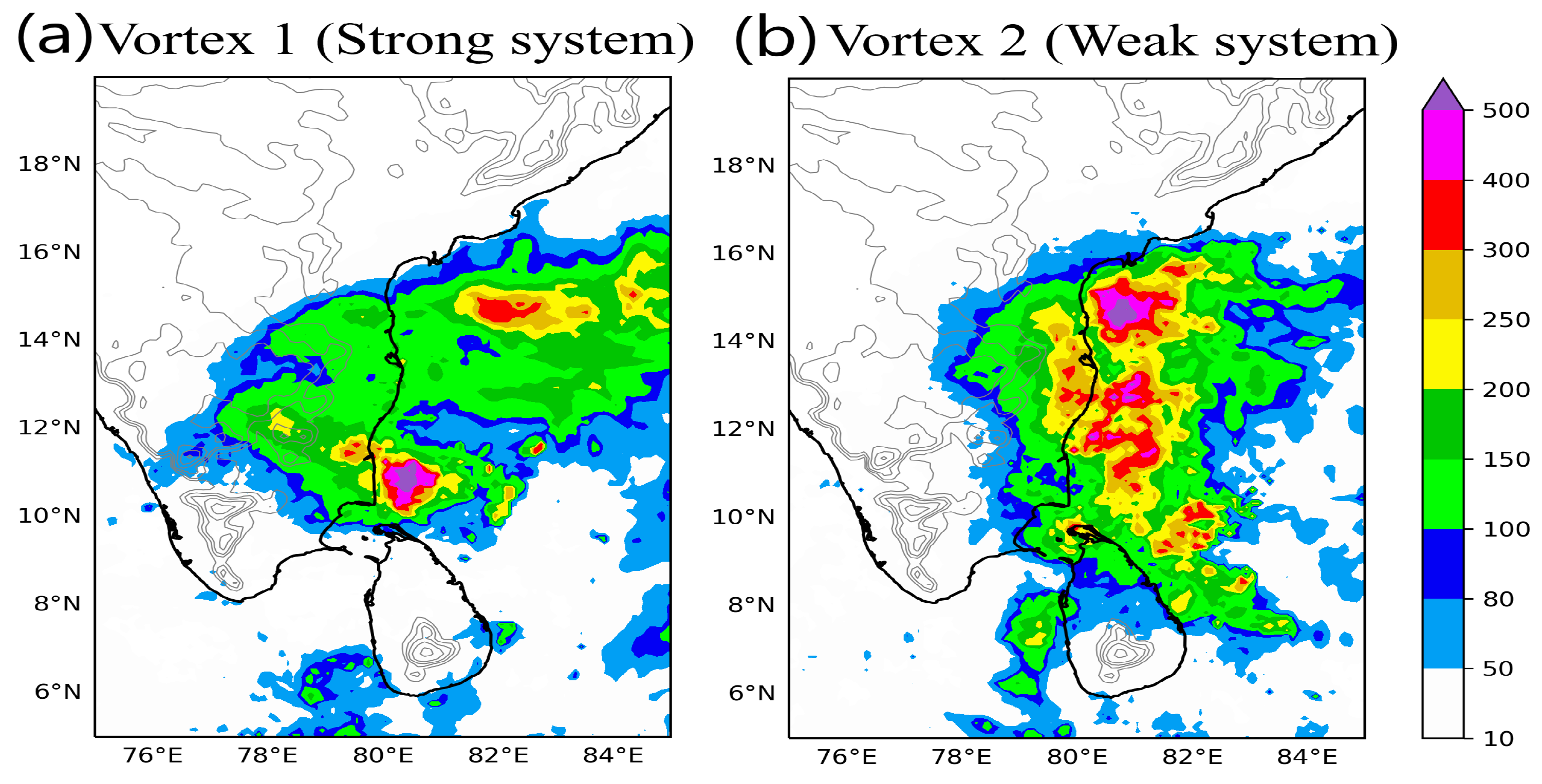
3.2. Convection and Rainfall

Figure 4 shows the IR brightness temperature images from the INSAT-3D satellite. Temperatures below 240 K are shown in colored shades to highlight the deep clouds. Convection in Vortex-1 spans a wider area; the western half of the vortex shows more deep clouds than the east (Figure 4a,b). Convection organization in the summer monsoon depressions over the northern Bay of Bengal was analyzed extensively, and the preference for the western half was attributed to the quasi-geostrophic ascent forced by the vertical shear [28,29,30,31,32,41,42]. Deep clouds led the path of Vortex-1 over the inland region. Convection in Vortex-2 stayed anchored over the coast for two consecutive days. It was better organized and larger than that in Vortex-1 on the second day (Figure 4c,d). The development of convection in Vortex-2 predominately occurred over the northern side of the vortex, i.e., where the onshore flow was likely to be influenced by the Eastern Ghats orography. The clouds were tallest over the offshore and coastal regions and shallow over the inland orographic region during both events.

The three-day rainfall accumulation associated with Vortex-1 and Vortex-2 is shown in Figure 5. In the case of Vortex-1, the coastal region received widespread heavy rainfall (>100 mm), localized severe rainfall (>200 mm ), and offshore extreme rainfall (>300 mm). The inland orographic region also received around 150–200 mm of rainfall. In the case of Vortex-2, the coastal region received widespread severe rainfall and the offshore region receives widespread extreme rainfall. Some onshore locations also receive rainfall over 300 mm. Thus, the coastal rainfall in Vortex-2 was more intense and widespread than in Vortex-1. The 300 m orographic contour separates the coastal region, which received rainfall greater than 200 mm, and the inland region, which is at a higher elevation, and received rainfall less than 150 mm during the Vortex-2 event.

In summary, Vortex-1 was stronger than Vortex-2 and moved swiftly across the Indian peninsula. However, convection in Vortex-2 remained organized for a longer duration than that in Vortex-1 while remaining over the Coromandel Coast. As a result, rainfall over the coastal region was much more severe in Vortex-2 and caused dangerous flooding on the ground. The rainfall contours run parallel to the topographic features in Vortex-2 (Figure 5b). Thus, the underlying topography seems to play an important role in the convective structure and overall dynamics of Vortex-2. Next, the vorticity budgets are studied to understand the underlying dynamics within these vortices.

4. Vorticity Budget

The propagation of vortices can be explained with the help of the vorticity budget. The vortex moves to the region where the vorticity budget gives maximum positive values. The vorticity budget in pressure coordinates can be written as follows [28,32,43]:

$$\frac{\partial \zeta }{\partial t}=-\underset{\mathrm{Stretching}}{\underbrace{\eta \nabla ·{\mathbf{u}}_{\mathbf{h}}}}-\underset{\mathrm{H}.\mathrm{Adv}}{\underbrace{{\mathbf{u}}_{\mathbf{h}}·\nabla \eta }}-\underset{\mathrm{V}.\mathrm{Adv}}{\underbrace{\omega \frac{\partial \zeta }{\partial p}}}+\underset{\mathrm{Tilting}}{\underbrace{\frac{\partial \omega }{\partial y}\frac{\partial u}{\partial p}-\frac{\partial \omega }{\partial x}\frac{\partial v}{\partial p}}}-\frac{\partial {\zeta }_{friction}}{\partial t}$$

(1)

where

$$\eta =\zeta +f$$

and $\zeta$ is relative vorticity, f the Coriolis parameter, $\eta$ absolute vorticity, ${\mathbf{u}}_{\mathbf{h}}$ horizontal flow vector, and $\omega$ vertical pressure velocity. The term ${\zeta }_{friction}$ denotes vorticity destruction due to surface friction. Note that the horizontal advection term can be written as follows:

$${\mathbf{u}}_{\mathbf{h}}·\nabla \eta ={\mathbf{u}}_{\mathbf{h}}·\nabla \zeta +\beta v$$

(2)

where $\beta$ = $\partial f/\partial y$. Thus, the horizontal advection term also includes the planetary $\beta$-effect. Although the $\left[\frac{\partial {\zeta }_{friction}}{\partial t}\right]$ term can be significant in the overall vorticity budget, it cannot be determined only with large-scale velocity fields, like the other terms in Equation (1). The following analysis includes only the stretching, advection, and tilting terms derived from the daily mean velocity fields of the ERA-interim. Therefore, the vorticity budget is not closed.

4.1. Vortex-1: Strong Vortex

Figure 6 shows plots for the daily vorticity tendency, stretching, horizontal and vertical advection, and tilting terms for Vortex-1 at 900 hPa during its crossover of the Indian peninsula. The 900 hPa level is considered, as the peak of orography lies around that height. A caveat to this analysis is that the roughness of rugged terrain will also destroy vorticity by increasing friction. However, this process is not considered here as it involves significant parameterization. The time tendency of relative vorticity ($\partial \zeta /\partial t$) is always positive on the western side of the vortex and negative on the eastern side, implying that Vortex-1 shifted to the west on subsequent days. The stretching and horizontal advection terms are more dominant than the other terms. The increase in vorticity by vortex stretching occurs over a large area within the vortex due to the low-level convergence induced by cyclonic circulation and topography (Figure 6b,g,l,q). The stretching term also coincides with the area of heavy rainfall around the vortex. This is not surprising as both quantities are the outcomes of convergence. It has consequences for the latent heat release in the vortex and the associated vorticity generation in the upper levels of the atmosphere (the bulk of it must occur over the low-level vortex stretching zone). On the other hand, the horizontal advection of vorticity has a dipole-like pattern before the landfall (Figure 6c,h). It is negative on the eastern side and approximately balances the vorticity increase due to stretching. It is positive over the western side and favors the westward propagation of the vortex. The vertical advection and tilting term are small, away from the orographic slopes. These terms become significant when the core of Vortex-1 is over the coast.

The vertical advection term is negative over the slopes of the Eastern Ghats where ascent occurs. This is due to the westward tilt in the vortex core as it approaches orography. The ascending flow has low vorticity compared to the air aloft due to the tilt (Figure 3). Similarly, the descending flow brings down high vorticity, and the vertical advection term is positive at these locations. The tilting term is positive over the orographic slopes and negative around the vortex center when it arrives near the orography (Figure 6j,o,t). This pattern arises due to the tilting of vorticity filaments over the orographic slopes, as shown in Figure 7.

The vertical shear of winds along the orographic slope (Figure 7b,c) creates horizontally oriented vorticity filaments, and the horizontal shear of the ascending flow (Figure 7a) helps in tilting these vorticity filaments (Figure 7d). Although the tilting term in the vorticity budget is generally small, it is quite large when Vortex-1 arrives near the orography and may help in overcoming the orographic barrier (Figure 6o). The ascent is the largest on the northern side of the vortex, where the onshore flow is uplifted by the orography. Thus, orography plays a significant role in the tilting of vorticity filaments. Note that negative $\omega$ is plotted in Figure 7a so that the ascending values are positive.

4.2. Vortex-2: Weak Vortex

Figure 8 shows the vorticity budget of Vortex-2. Vortex stretching is seen only on the upwind side to the orography where there is onshore flow as the vortex arrives over the coast (Figure 8g,l,q). Heavy rainfall contours of 100 and 200 mm are seen over the coast for three consecutive days (Figure 8b,g,l). Whereas, in the case of Vortex-1, heavy rainfall over the coast occurred for two consecutive days (Figure 6g,f). The pattern of the horizontal advection of vorticity is similar to Vortex-1 and it favors the westward progression of the vortex (Figure 8c,h,m,r). The vertical advection and tilting terms have similar patterns to Vortex-1 but are smaller in magnitude. This is due to the fact that weaker winds in Vortex-2 will produce weaker eddies and smaller vertical velocities over the orographic slopes. Thus, it can be hypothesized that the orography puts a barrier on the western side of the vortex, inducing convergence on the upwind side (this will be proved later with the help of sounding data). As a result, the vortex stretching happens only on the upwind side. The latent heat release (as seen from the rainfall accumulation) on the upwind side may also contribute to this.

Figure 9 shows vertical velocity and $\partial u/\partial p$, $\partial v/\partial p$ terms in Vortex-2 on 15 November. This date is chosen because the maximum tilting was seen on this day (Figure 8j). The ascent is weaker than that in Vortex-1 (Figure 7a). The distribution of the $\partial u/\partial p$ term is similar. However, the distribution of $\partial v/\partial p$ is different. It shows a negative gradient along the coast, i.e., the meridional wind speed decreases with increasing altitude at 900 hPa. This can be due to the formation of an orographic barrier jet over the coast. The presence of a barrier jet over the coast is shown later by analyzing the sounding data. As a result of this barrier jet, the tilting term is negative on the western side and unfavorable for the westward propagation of the vortex. The tilting is positive on the northern side of the vortex and it results from the increase in zonal winds with altitude (Figure 9b). However, the magnitude of this tilting is weaker than that seen in Vortex-1 due to a weaker ascent.

Although the tilting and vertical advection are significant over the orography, the stretching and horizontal advection are the dominant mechanisms, in terms of intensity and expanse, in both vortices. Therefore, the vertical distribution of vortex stretching and horizontal advection is analyzed next to understand how the orographic influence is felt at the upper levels.

As Vortex-1 approaches the coast, vortex stretching predominately occurs in the lower troposphere and within the layer adjacent to the orography (Figure 10a,c,e). In this case, the vortex stretching also occurs over the orographic slope on 10 and 11 November as Vortex-1 moves across the peninsula (Figure 10c,e). The east–west dipole in the horizontal vorticity advection is seen in the entire depth of the vortex on most days, even as the vortex crosses the orographic barrier (Figure 10b,f,h). The prominent difference between the vertical structures of the vorticity budget of the two vortices can be seen in the vortex stretching term near the orography. In the case of Vortex-2, vortex stretching always occurs upstream of the orography (Figure 11a,c,e,g); a clear gap between the positive vortex stretching and the orographic slope can be seen. The vorticity and vortex stretching contours align with the orographic slope ahead of it. This can be due to the upstream orographic blocking and piling up of a cold pool of air as shown by Phadtare [10]. As a result, Vortex-2 remains upstream of the orography. To prove the orographic blocking phenomenon, sounding data from Chennai are analyzed next.

4.3. Orographic Blocking

Figure 12 shows the vertical profiles of winds over the coast from the radiosonde soundings over Chennai at 1200 UTC 09 November (Vortex-1) and at 1200 UTC 15 November (Vortex-2). The winds are stronger in the lower troposphere on 9 November. In both cases, winds are easterlies in the lower free troposphere. However, on 15 November, winds abruptly changed direction and became northeasterlies below 1000 m altitude. This height is roughly equal to the elevation of orography. Thus, this deflection seems to be caused by the orographic barrier. A barrier jet is seen just below this level in Figure 12b on 15 November. The presence of a barrier jet was hypothesized in Figure 9c and was blamed for the negative vortex tilting along the coast.

Winds on 9 November are easterly throughout, including the boundary layer and, hence, are undeflected by the orographic barrier. The orographic blocking of the flow is determined by its Froude number [44]:

$$F=U/NH$$

(3)

where U is the mean wind speed, N is the mean Brunt Väisälä frequency over the orographic height H. When F is below 1, the flow is blocked by the orographic barrier, and vice versa. On 9 November (Vortex-1), the F of the flow was 1.2 (U = 12 m s${}^{-1}$, N = 0.013 s${}^{-1}$, H = 750 m), and on 15 November, it was 0.77 (U = 7.5 m s${}^{-1}$, N = 0.013 s${}^{-1}$, H = 750 m). Thus, the flow on 15 November was not strong enough to cross the orographic barrier and got deflected forming a barrier jet, as seen in Figure 11. The coastal flow on 9 November remained undeflected as its F value was greater than 1.

5. Conclusions and Discussion

The motivation behind this study was to highlight the likely severity of weak cyclonic systems and decipher the underlying mechanism behind their quasi-stationarity along the east coast of India. The propagation of two post-monsoon cyclonic systems over peninsular India was studied by analyzing their vorticity budgets at 900 hPa. The following are the main conclusions of this study:

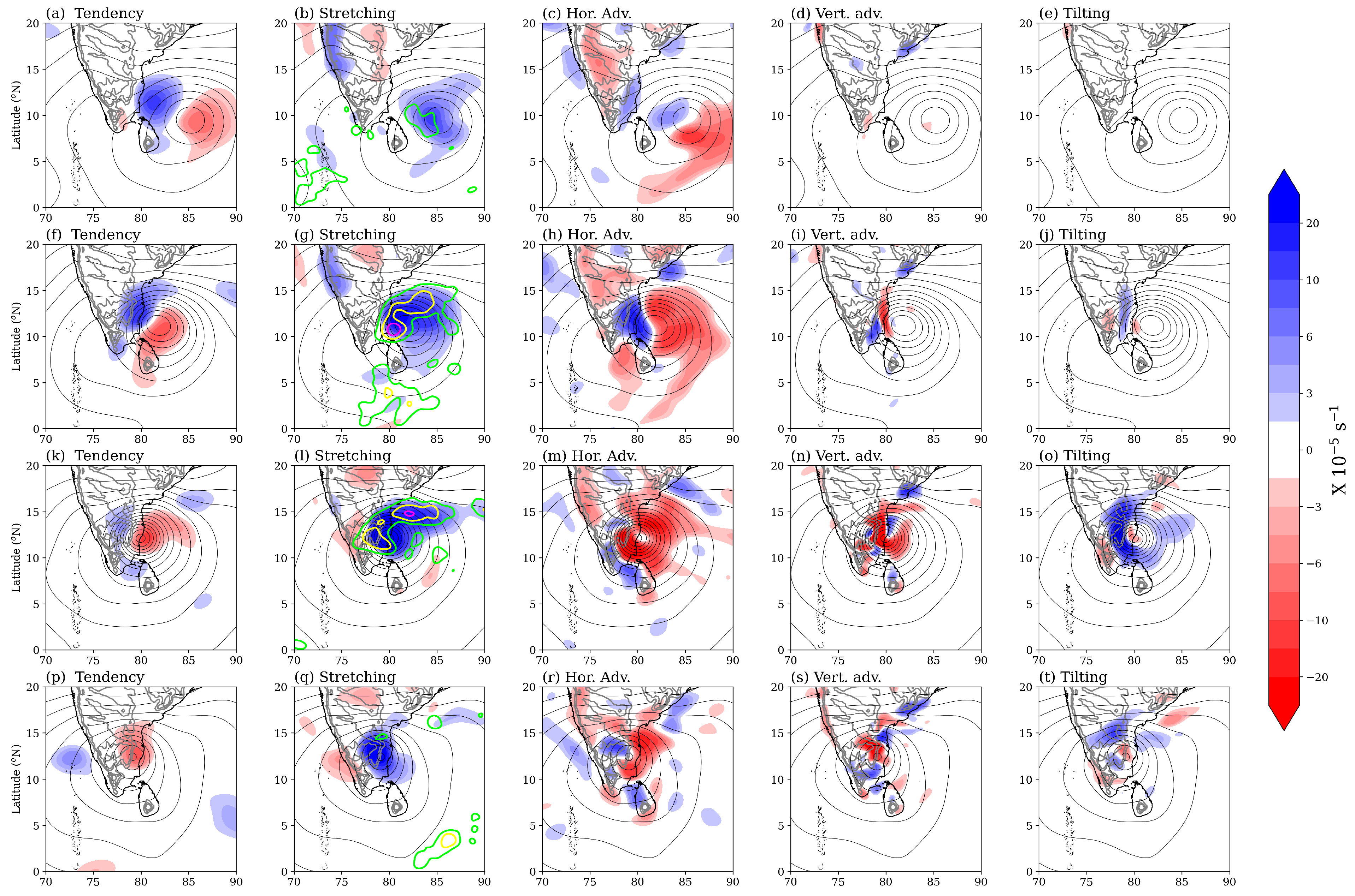
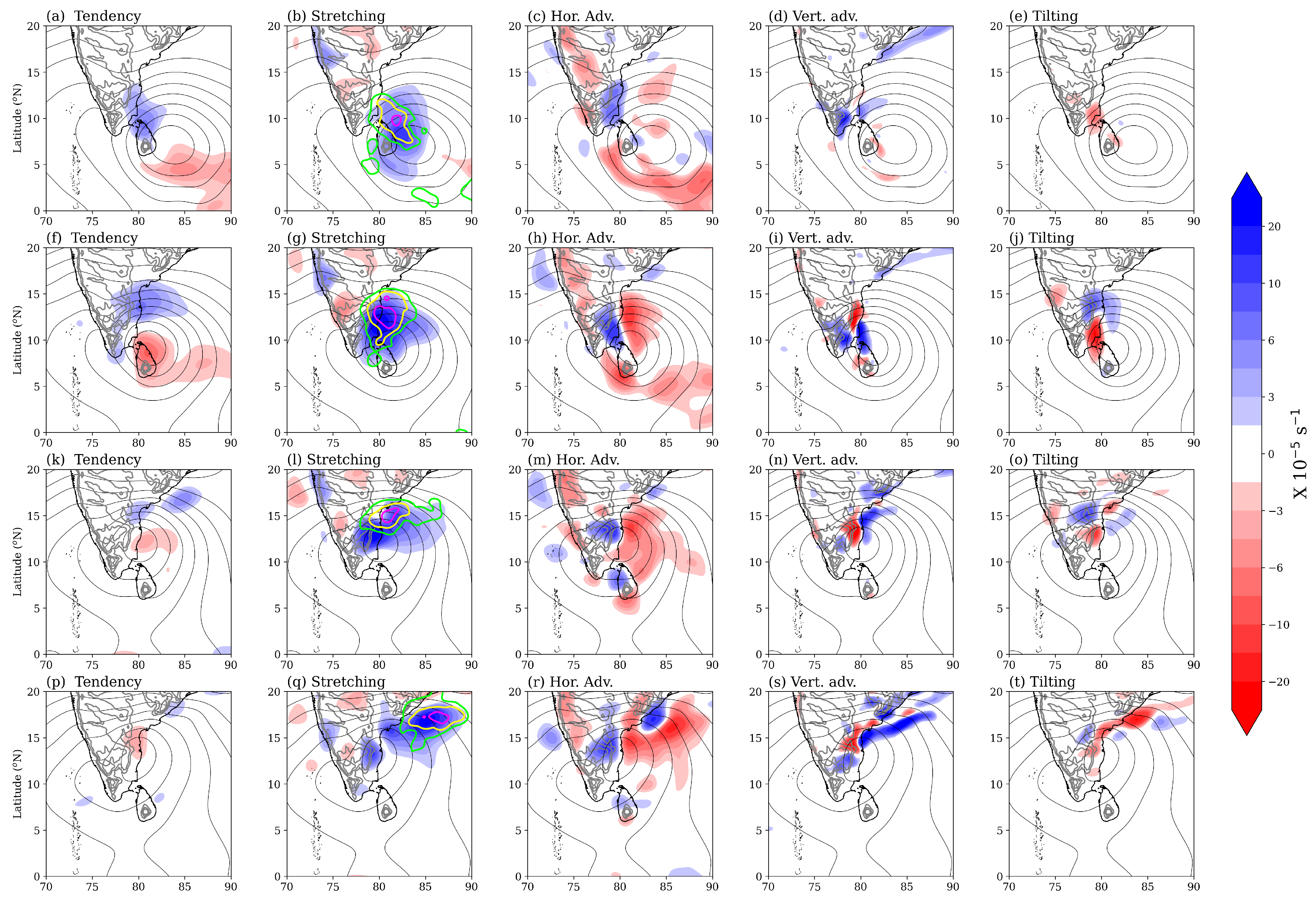
• Vortex stretching and horizontal advection were the dominant terms in the vorticity budgets of these vortices. The horizontal vorticity advection was positive on the western side and negative on the eastern side of the vortices. This dipole favored the westward progression of the vortices.
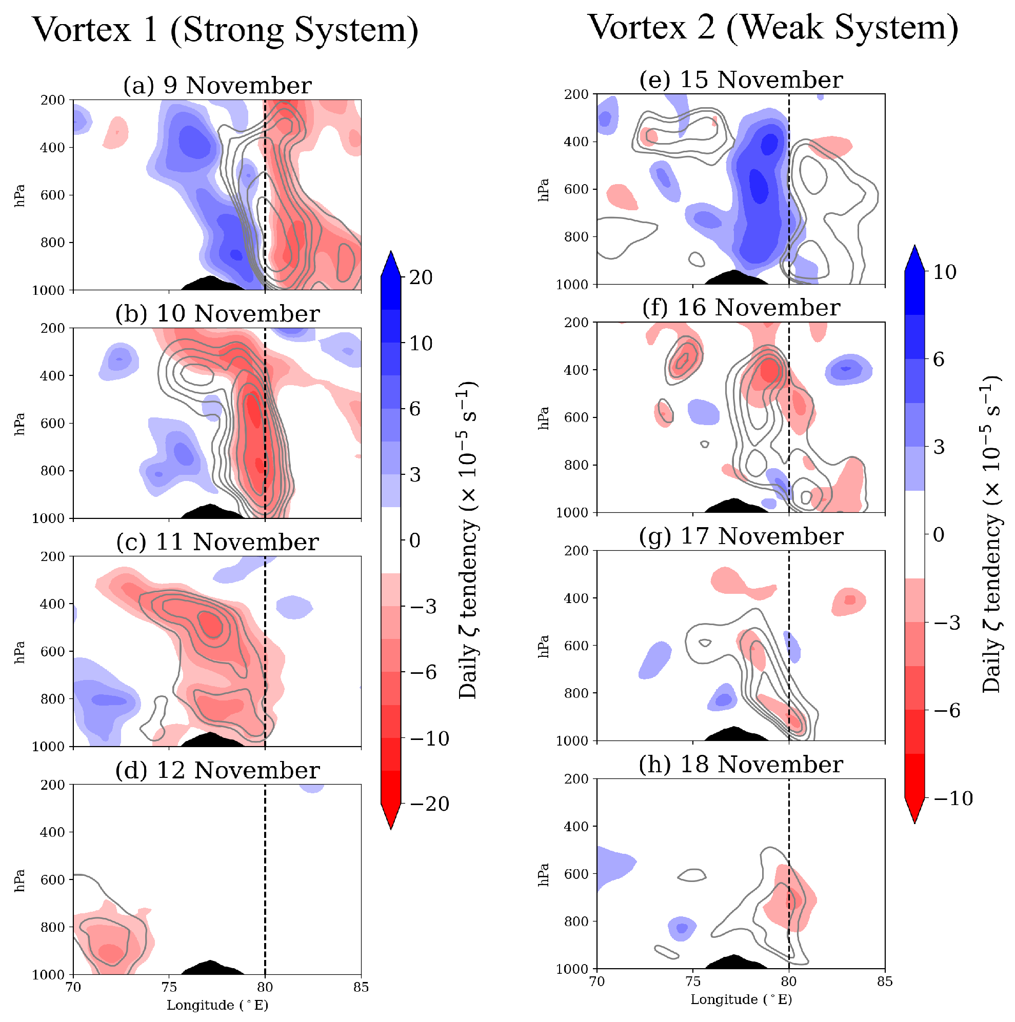
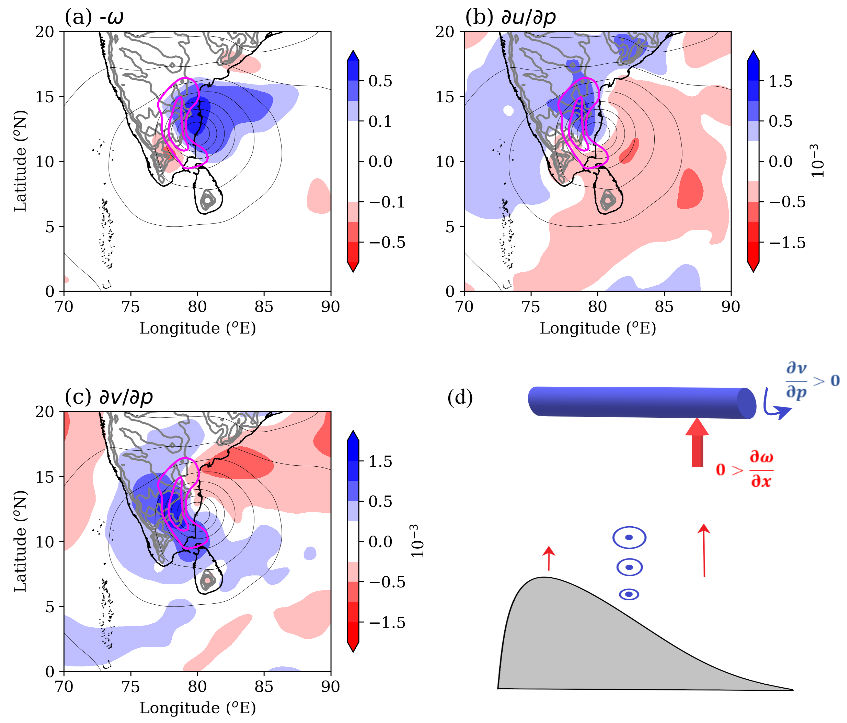
• The vertical advection of vorticity was significant only over the orographic slope. This quantity was negative in the ascending zone and positive in the descending zone due to the westward tilt of the vortex near the orography.
• The tilting of the vorticity filaments was stronger in Vortex-1 due to the stronger ascent over the coast. This resulted in a cyclonic vorticity tendency due to tilting over the orographic slopes in Vortex-1. In the case of (the weaker) Vortex-2, the vorticity filaments were tilted due to the barrier jet in a manner so that an anticyclonic vorticity tendency appeared over the orographic slope on the western side of the vortex.
• The vortex stretching always occurred upstream of the orography in Vortex-2 due to the convergence caused by upstream orographic blocking. Hence, Vortex-2 remained upstream of the orography. The stronger winds in Vortex-1 resulted in convergence and vortex stretching over the orography, notwithstanding its barrier effect. Therefore, Vortex-1 moved over the orography swiftly.

The weaker system stalled along the east coast, causing widespread intense rainfall and severe flooding. Weaker systems have weaker winds, which may initially appear innocuous on weather maps. Nevertheless, they are generally slow-moving as their vortex drift speeds ($v_d$∝${\mathbf{u}}_{\mathbf{h}}·\nabla \eta$) are small [3]. These slow-moving vortices can dump heavy rainfall for a long duration over an area. The topographic barrier cannot only obstruct their westward propagation but also better organize convection in these systems by providing a mechanical uplift to the air parcels with high conditional instability [10]. Although this study presents only two cases, it provides a motivation for studying the climatological pattern of vortex stalling along the Coromandel Coast. The stationary cyclonic vortex during the 1–4 December 2015 flooding event also showed a vorticity budget similar to Vortex-2 (not included here). The typical life cycle of stalled systems should be studied so that their forecasting is improved. The following hypothesis can be made, considering the findings of this study: a non-dimensional vortex Froude number $F_v$, where U in Equation (3) is replaced by the maximum radial wind speed of the cyclonic system, can be used to predict the stalling of a vortex along the coast. The climatological study will also be helpful in testing this hypothesis. This requires an automated tracking of cyclonic systems [45,46,47,48] and, hence, a separate research article for the climatological study is justified.

Another limitation of this analysis is the exclusion of convective organization and its effect on the overall dynamics of the vortex. How convection organizes within these systems and how it affects the overall vorticity budget needs to be addressed. Vertical coupling in these vortices seems to be achieved via convection as the vorticity budget is affected by vertical advection. Thus, the orographic influence can be relayed to the upper levels by convection. This aspect was not looked into and can be studied in the future, perhaps with numerical models.

As far as the general circulation models (GCMs) are concerned, how well the operational GCMs capture the stalling of a vortex should be investigated. This can be a challenging task for GCMs as the stalling may depend on the details of topography–convection interaction and GCMs in which convection and boundary layer processes are parameterized may miss these details. Therefore, forecasting the stalling of cyclonic systems may also require human judgment and the climatological study will be helpful in this aspect as well.

References

1. Charney, J.G.; Eliassen, A. On the growth of the hurricane depression. J. Atmos. Sci. 1964, 21, 68–75. [Google Scholar] [CrossRef]
2. Chan, J.C.; Williams, R. Analytical and numerical studies of the beta-effect in tropical cyclone motion. Part I: Zero mean flow. J. Atmos. Sci. 1987, 44, 1257–1265. [Google Scholar] [CrossRef]
3. Fiorino, M.; Elsberry, R.L. Some aspects of vortex structure related to tropical cyclone motion. J. Atmos. Sci. 1989, 46, 975–990. [Google Scholar] [CrossRef]
4. Wang, Y.; Wu, C.C. Current understanding of tropical cyclone structure and intensity changes—A review. Meteorl. Atmos. Phys. 2004, 87, 257–278. [Google Scholar] [CrossRef]
5. Chan, J.C. The physics of tropical cyclone motion. Annu. Rev. Fluid Mech. 2005, 37, 99–128. [Google Scholar] [CrossRef]
6. Tamarin, T.; Kaspi, Y. The poleward motion of extratropical cyclones from a potential vorticity tendency analysis. J. Atmos. Sci. 2016, 73, 1687–1707. [Google Scholar] [CrossRef]
7. Sengupta, D.; Goddalehundi, B.R.; Anitha, D. Cyclone-induced mixing does not cool SST in the post-monsoon North Bay of Bengal. Atmos. Sci. Lett. 2008, 9, 1–6. [Google Scholar] [CrossRef]
8. Van Oldenborgh, G.J.; Van Der Wiel, K.; Sebastian, A.; Singh, R.; Arrighi, J.; Otto, F.; Haustein, K.; Li, S.; Vecchi, G.; Cullen, H. Attribution of extreme rainfall from Hurricane Harvey, August 2017. Environ. Res. Lett. 2017, 12, 124009. [Google Scholar] [CrossRef]
9. Chakraborty, A. A synoptic-scale perspective of heavy rainfall over Chennai in November 2015. Curr. Sci. 2016, 111, 201–207. [Google Scholar] [CrossRef]
10. Phadtare, J. Role of Eastern Ghats Orography and Cold Pool in an Extreme Rainfall Event over Chennai on 1 December 2015. Mon. Weather Rev. 2018, 146, 943–965. [Google Scholar] [CrossRef]
11. Stevens, J.; Carlowicz, M. Historic Rainfall Floods Southeast India. 2015. Available online: https://earthobservatory.nasa.gov/images/87131/historic-rainfall-floods-southeast-india (accessed on 12 March 2023).
12. Boyaj, A.; Ashok, K.; Ghosh, S.; Devanand, A.; Dandu, G. The Chennai extreme rainfall event in 2015: The Bay of Bengal connection. Clim. Dyn. 2018, 50, 2867–2879. [Google Scholar] [CrossRef]
13. Zubair, L.; Ropelewski, C.F. The strengthening relationship between ENSO and northeast monsoon rainfall over Sri Lanka and southern India. J. Clim. 2006, 19, 1567–1575. [Google Scholar] [CrossRef] [Green Version]
14. Kumar, P.; Kumar, K.R.; Rajeevan, M.; Sahai, A. On the recent strengthening of the relationship between ENSO and northeast monsoon rainfall over South Asia. Clim. Dyn. 2007, 28, 649–660. [Google Scholar] [CrossRef]
15. Geethalakshmi, V.; Yatagai, A.; Palanisamy, K.; Umetsu, C. Impact of ENSO and the Indian Ocean Dipole on the north-east monsoon rainfall of Tamil Nadu State in India. Hydrol. Process. Int. J. 2009, 23, 633–647. [Google Scholar] [CrossRef]
16. Yadav, R. Why is ENSO influencing Indian northeast monsoon in the recent decades? Int. J. Climatol. 2012, 32, 2163–2180. [Google Scholar] [CrossRef]
17. Rajeevan, M.; Unnikrishnan, C.; Bhate, J.; Niranjan Kumar, K.; Sreekala, P. Northeast monsoon over India: Variability and prediction. Meteorol. Appl. 2012, 19, 226–236. [Google Scholar] [CrossRef]
18. Sreekala, P.; Rao, S.V.B.; Rajeevan, M. Northeast monsoon rainfall variability over south peninsular India and its teleconnections. Theor. Appl. Climatol. 2012, 108, 73–83. [Google Scholar] [CrossRef]
19. Krishnamurthy, L.; Vecchi, G.A.; Yang, X.; van der Wiel, K.; Balaji, V.; Kapnick, S.B.; Jia, L.; Zeng, F.; Paffendorf, K.; Underwood, S. Causes and probability of occurrence of extreme precipitation events like Chennai 2015. J. Clim. 2018, 31, 3831–3848. [Google Scholar] [CrossRef]
20. van Oldenborgh, G.; Otto, F.; Haustein, K.; Achuta Rao, K. The heavy precipitation event of December 2015 in Chennai, India. B Am. Meteorol. Soc. 2016, 97, S87–S91. [Google Scholar] [CrossRef] [Green Version]
21. Leroux, M.D.; Wood, K.; Elsberry, R.; Cayanan, E.; Hendricks, E.; Kucas, M.; Otto, P.; Rogers, R.; Sampson, B.; Yu, Z. Recent Advances in Research and Forecasting of Tropical Cyclone Track, Intensity, and Structure at Landfall. Trop. Cyclone Res. Rev. 2018, 7, 85–105. [Google Scholar] [CrossRef]
22. Vaidya, S.; Mukhopadhyay, P.; Trivedi, D.; Sanjay, J.; Singh, S. Prediction of tropical systems over Indian region using mesoscale model. Meteorl. Atmos. Phys. 2004, 86, 63–72. [Google Scholar] [CrossRef]
23. Mohapatra, M.; Nayak, D.; Sharma, R.; Bandyopadhyay, B. Evaluation of official tropical cyclone track forecast over north Indian Ocean issued by India Meteorological Department. J. Earth Syst. Sci. 2013, 122, 589–601. [Google Scholar] [CrossRef] [Green Version]
24. Osuri, K.K.; Mohanty, U.; Routray, A.; Niyogi, D. Improved prediction of Bay of Bengal tropical cyclones through assimilation of Doppler weather radar observations. Mon. Weather Rev. 2015, 143, 4533–4560. [Google Scholar] [CrossRef]
25. Mohanty, U.; Osuri, K.K.; Pattanayak, S. Tropical Cyclone Research over the North Indian Ocean: Impact of Data and Vortex Initialization in High Resolution Mesoscale Models. In Advanced Numerical Modeling and Data Assimilation Techniques for Tropical Cyclone Prediction; Springer Dordrecht: Berlin/Heidelberg, Germany, 2016; pp. 465–495. [Google Scholar] [CrossRef]
26. Kumkar, Y.V.; Sen, P.; Chaudhari, H.S.; Oh, J.H. Tropical cyclones over the North Indian Ocean: Experiments with the high-resolution global icosahedral grid point model GME. Meteorl. Atmos. Phys. 2018, 130, 23–37. [Google Scholar] [CrossRef]
27. Routray, A.; Dutta, D.; George, J.P. Evaluation of Track and Intensity Prediction of Tropical Cyclones Over North Indian Ocean Using NCUM Global Model. Pure Appl. Geophys. 2018, 176, 421–440. [Google Scholar] [CrossRef]
28. Daggupaty, S.M.; Sikka, D.R. On the vorticity budget and vertical velocity distribution associated with the life cycle of a monsoon depression. J. Atmos. Sci. 1977, 34, 773–792. [Google Scholar] [CrossRef]
29. Sanders, F. Quasi-geostrophic diagnosis of the monsoon depression of 5–8 July 1979. J. Atmos. Sci. 1984, 41, 538–552. [Google Scholar] [CrossRef]
30. Douglas, M.W. Structure and dynamics of two monsoon depressions. Part I: Observed structure. Mon. Weather Rev. 1992, 120, 1524–1547. [Google Scholar] [CrossRef]
31. Chen, T.C.; Yoon, J.H.; Wang, S.Y. Westward propagation of the Indian monsoon depression. Tellus A Dyn. Meteorol. Oceanogr. 2005, 57, 758–769. [Google Scholar] [CrossRef]
32. Boos, W.; Hurley, J.; Murthy, V. Adiabatic westward drift of Indian monsoon depressions. Q. J. R. Meteorol. Soc. 2015, 141, 1035–1048. [Google Scholar] [CrossRef] [Green Version]
33. Raymond, D.; Jiang, H. A theory for long-lived mesoscale convective systems. J. Atmos. Sci. 1990, 47, 3067–3077. [Google Scholar] [CrossRef]
34. Stoelinga, M.T. A potential vorticity-based study of the role of diabatic heating and friction in a numerically simulated baroclinic cyclone. Mon. Weather Rev. 1996, 124, 849–874. [Google Scholar] [CrossRef]
35. Zehnder, J.A. The influence of large-scale topography on barotropic vortex motion. J. Atmos. Sci. 1993, 50, 2519–2532. [Google Scholar] [CrossRef]
36. Harold, F.P.; Gutro, R. NASA Measures India’s Deadly Flooding Rains. 2015. Available online: https://www.nasa.gov/feature/goddard/97b-north-indian-ocean (accessed on 12 March 2023).
37. Hersbach, H.; Bell, B.; Berrisford, P.; Biavati, G.; Horányi, A.; Muñoz Sabater, J.; Nicolas, J.; Peubey, C.; Radu, R.; Rozum, I.; et al. ERA5 Hourly Data on Pressure Levels from 1979 to Present. Copernicus Climate Change Service (C3S) Climate Data Store (CDS). 2018. Available online: https://cds.climate.copernicus.eu/ (accessed on 12 November 2022).
38. Pierrehumbert, R.; Wyman, B. Upstream effects of mesoscale mountains. J. Atmos. Sci. 1985, 42, 977–1003. [Google Scholar] [CrossRef]
39. Phadtare, J.A.; Fletcher, J.K.; Ross, A.N.; Turner, A.G.; Schiemann, R.K. Froude-number-based rainfall regimes over the Western Ghats mountains of India. Q. J. R. Meteorol. Soc. 2022, 148, 3388–3405. [Google Scholar] [CrossRef]
40. Huffman, G.J.; Bolvin, D.T.; Nelkin, E.J.; Tan, J. Integrated Multi-satellitE Retrievals for GPM (IMERG) technical documentation. NASA/GSFC Code 2015, 612, 2019. [Google Scholar]
41. Adames, Á.F.; Ming, Y. Interactions between water vapor and potential vorticity in synoptic-scale monsoonal disturbances: Moisture vortex instability. J. Atmos. Sci. 2018, 75, 2083–2106. [Google Scholar] [CrossRef]
42. Phadtare, J.; Bhat, G. Characteristics of deep cloud systems under weak and strong synoptic forcing during the Indian summer monsoon season. Mon. Weather Rev. 2019, 147, 3741–3758. [Google Scholar] [CrossRef]
43. Holton, J.R.; Hakim, G.J. Circulation, Vorticity, and Potential Vorticity. In An Introduction to Dynamic Meteorology, 5th ed.; Academic Press: Cambridge, MA, USA, 2013; pp. 95–125. [Google Scholar]
44. Lin, Y.L.; Wang, T.A. Flow regimes and transient dynamics of two-dimensional stratified flow over an isolated mountain ridge. J. Atmos. Sci. 1996, 53, 139–158. [Google Scholar] [CrossRef]
45. Hurley, J.V.; Boos, W.R. A global climatology of monsoon low-pressure systems. Q. J. R. Meteorol. Soc. 2015, 141, 1049–1064. [Google Scholar] [CrossRef] [Green Version]
46. Hunt, K.M.; Turner, A.G.; Inness, P.M.; Parker, D.E.; Levine, R.C. On the structure and dynamics of Indian monsoon depressions. Mon. Weather Rev. 2016, 144, 3391–3416. [Google Scholar] [CrossRef] [Green Version]
47. Kushwaha, P.; Sukhatme, J.; Nanjundiah, R. A Global Tropical Survey of Midtropospheric Cyclones. Mon. Weather Rev. 2021, 149, 2737–2753. [Google Scholar] [CrossRef]
48. Thomas, T.M.; Bala, G.; Srinivas, V.V. Characteristics of the monsoon low pressure systems in the Indian subcontinent and the associated extreme precipitation events. Clim. Dyn. 2021, 56, 1859–1878. [Google Scholar] [CrossRef]
Figure 1. Topography of part of South Asia. A hypothetical cyclonic storm is sketched in black concentric circles and its northwestward β -drift is shown by a dashed line.
Meteorology 02 00020 g001
Figure 2. The 900 hPa wind speed (shading) and geopotential height contours (maximum = 1000 m, decreasing by 5 m intervals) from ERA5 at 0000 UTC (a) 8 November, (b) 9 November, (c) 10 November, (d) 11 November, (e) 14 November, (f) 15 November, (g) 16 and (h) 17 November 2015.
Meteorology 02 00020 g002
Figure 3. Daily mean relative vorticity ( ζ ) contours (2, 3, 5, 8, and 10 × 10 5 s 1 ) and ζ -tendency (shading) averaged over the 8–15 N zonal band. (ad) Vortex-1: 9–12 November, and (eh) Vortex-2: 15–18 November 2015. The vertical dashed line shows the mean location of the Coromandel Coast.
Meteorology 02 00020 g003
Figure 4. IR brightness temperature from the INSAT-3D satellite. Vortex-1: (a) 0000 UTC 9 November, (b) 0000 UTC 10 November, and Vortex-2: (c) 0000 UTC 15 November, and (d) 0000 UTC 16 November 2015.
Meteorology 02 00020 g004
Figure 5. Three-Day rainfall accumulation from IMERG product. (a) Vortex-1: 0000 UTC 8 November–0000 UTC 11 November, and (b) Vortex-2: 0000 UTC 14 November–0000 UTC 17 November 2015. The light gray contours show 300, 500, 750, 1000, 1500, and 2000 m elevation.
Meteorology 02 00020 g005
Figure 6. Daily means of the terms in the vorticity budget, given by Equation (1), calculated from the ERA5 data (shading) at 900 hPa. Geopotential height contours (5 m intervals) at the same level are overlaid. (a) Time tendency, (b) stretching, (c) horizontal advection, (d) vertical advection, and (e) tilting of relative vorticity ( ζ ) on 7 November 2015. (ft) The same as (ae) but on 8, 9, and 10 November 2015, respectively. The green, yellow, and magenta contours on the stretching term show daily rainfall, with values of 50, 100, and 200 mm, respectively, from IMERG.
Meteorology 02 00020 g006
Figure 7. Mean (a) - ω , (b) u / p , and (c) v / p at 900 hPa on 10 November 2015 from ERA5. The magenta contours in (ac) show vortex tilting with 5 and 20 × 10 5 s 1 values. (d) A schematic for the orography-induced vortex tilting (Equation (1)) in the longitude-pressure plane ( v p ω x term). The blue cylinder shows the rotation of vorticity filaments and the thick red arrow shows its tilting due to ω / x .
Meteorology 02 00020 g007
Figure 8. The same as Figure 6 but for (ae) 14 November, (fj) 15 November, (ko) 16 November, and (pt) 17 November 2015.
Meteorology 02 00020 g008
Figure 9. Mean (a) - ω , (b) u / p , and (c) v / p at 900 hPa on 15 November 2015 from ERA5. The magenta contours show vortex tilting with 5 × 10 5 s 1 value.
Meteorology 02 00020 g009
Figure 10. (a) Mean relative vorticity ( ζ ) contours (2, 3, 5, 8, and 10 × 10 5 s 1 ) and vortex stretching term (shading) averaged over 8–15 N zonal band, and (b) same as (a) but for the horizontal vorticity advection term on 9 November; (ch) are the same as (a,b) but for 10, 11, and 12 November, respectively. The vertical dashed line shows the mean location of the Coromandel Coast.
Meteorology 02 00020 g010
Figure 11. The same as Figure 9 but for (a,b) 15, (c,d) 16, (e,f) 17, and (g,h) 18 November.
Meteorology 02 00020 g011
Figure 12. (a) Wind speed and (b) wind direction from the radiosondes over Chennai on 9 November and 15 November 2015. The horizontal dashed line shows the mean elevation of the Eastern Ghats (750 m).
Meteorology 02 00020 g012
Disclaimer/Publisher’s Note: The statements, opinions and data contained in all publications are solely those of the individual author(s) and contributor(s) and not of MDPI and/or the editor(s). MDPI and/or the editor(s) disclaim responsibility for any injury to people or property resulting from any ideas, methods, instructions or products referred to in the content.