
The Impact of Ice Formation on Vertical Axis Wind Turbine Performance and Aerodynamics


School of Engineering, Robert Gordon University, Aberdeen AB10 7GJ, UK
*
Author to whom correspondence should be addressed.
Wind 2023, 3(1), 16-34; https://doi.org/10.3390/wind3010003
Submission received: 7 December 2022
/
Revised: 8 January 2023
/
Accepted: 17 January 2023
/
Published: 27 January 2023
(This article belongs to the Special Issue Challenges and Perspectives of Wind Energy Technology)
Abstract
:This study investigated the impact of ice formation on the performance and aerodynamics of a vertical axis wind turbine (VAWT). This is an area that is becoming more prevalent as VAWTs are installed alongside horizontal axis wind turbines (HAWTs) in high altitude areas with cold and wet climates where ice is likely to form. Computational fluid dynamics (CFD) simulations were performed on a VAWT without icing in Ansys to understand its performance before introducing ice shapes obtained through the LewInt ice accretion software and repeating simulations in Ansys. These simulations were verified by performing a wind tunnel experiment on a scale VAWT model with and without 3D printed ice shapes attached to the blades. The clean blade simulations found that wind speed had little impact on the performance, while reducing the blade scale severely reduced performance. The ice formation simulations found that increasing the icing time or liquid water content (LWC) led to increased ice thickness. Additionally, glaze ice and rime ice conditions were investigated, and it was found that rime ice conditions that occur in lower temperatures caused more ice to form. The simulations with the attached ice shapes found a maximum reduction in performance of 40%, and the experiments found that the ice shapes made the VAWT unable to produce power.
1. Introduction
Renewable energy is becoming an ever more essential energy source as the world transitions away from fossil fuels and towards a carbon-free future. One such renewable energy source that has seen a large amount of implementation and success is wind energy, with onshore and offshore wind producing 23.2 TWh of energy in Scotland from 2000–2020 [1]. The current production of wind energy comes from wind farms containing horizontal axis wind turbines (HAWTs), as they have had much more research done on their ability to harvest energy, along with more success in the research; thus, they have dominated the market for wind energy. However, HAWTs require tall structures that leave wind energy closer to the ground unharvested. One method to prevent this is installing vertical axis wind turbines (VAWTs) alongside HAWTs, as VAWTs can harvest energy low to the ground, leading to mixed windfarms using HAWTs and VAWTs.
For these mixed wind farms to be successfully implemented, VAWTs will have to be able to withstand and operate efficiently in similar conditions to HAWTs. This includes cold and wet climates, especially those at high altitudes such as the Swiss Alps and many areas in China and North America, which often have high wind speeds and therefore have a lot of wind energy available to harvest. However, these climates also lead to the formation of ice on exposed surfaces such as wind turbine blades. This formation of ice can lead to the efficiency of the turbines dropping, leaving more energy unharvested and increasing the cost of operation associated with the turbines.
A lot of research has been done into the impact of icing on the performance and aerodynamics of HAWTs; however, the same cannot be said about VAWTs where there is a lack of research into this area. The lack of research for VAWTs is the reason for this, which will investigate the impact of ice formation on the performance and aerodynamics of a VAWT through computational fluid dynamics (CFD) and experiments. This report will use simulations and experiments to investigate performance and aerodynamics of the VAWT while it is rotating as opposed to a static turbine as is often investigated. Rotating VAWTs have been investigated; however, there was little to no research found that is combined with ice formation on the VAWT.
This report will begin with an overview of relevant literature in Section 2. Section 3 will cover the methodology for both the numerical and experimental work that was performed. Section 4 discusses the results from the clean blade simulations, and Section 5 discusses the results from the icing simulations. Lastly, Section 6 discusses the results from both the clean blade and icing experiments, followed by a summary of the conclusions and recommendations in Section 7.
2. Background
2.1. VAWTs
VAWTs are turbines that consist of blades that rotate around a vertical axis. This allows VAWTs to be designed to operate close to the ground, as blade clearance is not required, allowing them to be used in urban areas without causing as much disruption as a HAWT would.
The performance of a VAWT is determined by comparing the power it can produce to the power available from the wind in the turbine area, as can be seen in Equation (1).
The power available in the wind can be obtained using Equation (2) and is a function of the air density, area, and the wind velocity. The power generated by the VAWT can be obtained using Equation (3) and is a function of the moment acting on the blades and the rotational speed of the turbine.
However, the moment is rarely used and is often replaced with a non-dimensional moment coefficient, Equation (4). This is used alongside the tip speed ratio (TSR), Equation (5), which is a key parameter in VAWT design to obtain a coefficient of performance, Equation (6).
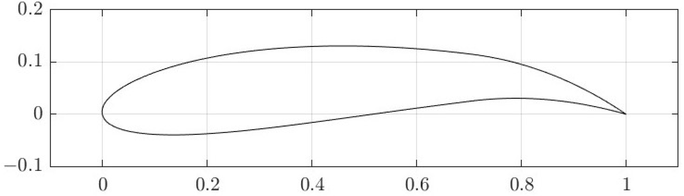
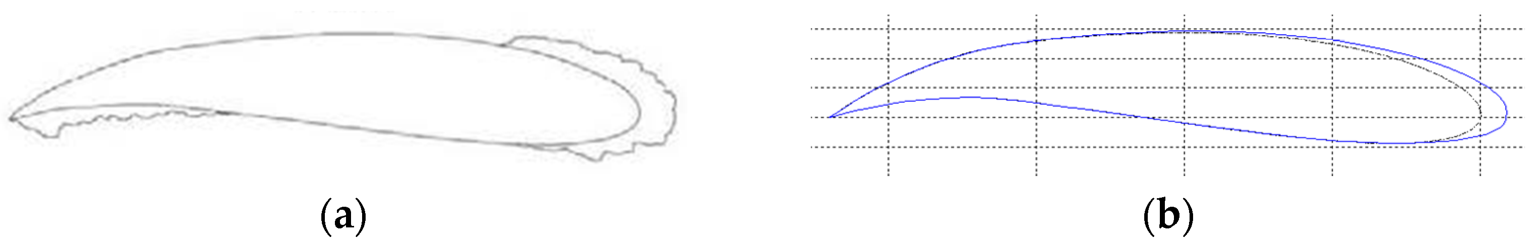
The performance of a VAWT can be optimized by altering design parameters such as the radius of the turbine, the number of blades, the shape of the blades, etc. Codes such as NACA have been created to classify blades based on their shape following the format of NACA MPXX where M is the maximum camber divided by 100, P is the position of maximum camber divided by 10, and XX is the thickness divided by 100 [2]. The aerofoil that will be the subject of this report is the NACA 7715 shown in Figure 1.
Altering the shape of this aerofoil will change how much drag the turbine experiences and how much lift is produced, allowing performance to be improved. Performance improvement has also been achieved by altering the flow of wind using upstream deflectors [3] or planetary turbines [4]. Both studies found about 1% improvement in efficiency over a traditional VAWT.
2.2. Ice Formation
In certain meteorological conditions, when water droplets encounter a surface, the droplets will freeze and form ice. The type of ice that forms depends on these conditions and can be categorized as rime or glaze ice. Rime ice forms as a rough, opaque shape, making it easy to identify, and occurs when droplets freeze rapidly upon impacting a surface. Glaze ice, also referred to as clear ice, forms when only part of a droplet freezes when impacting a surface, causing the remaining water to spread over the surface. This causes the ice to be clear, making it hard to spot. Glaze ice primarily forms in temperatures between 0 °C and −10 °C [5]. A mix of rime and glaze ice can also occur.
The severity of Ice formations depends on three main variables: the liquid water content (LWC), the temperature, and the droplet size. LWC is a measure of how much water there is in a given volume of air, describing how wet the conditions are. LWC in air has been classified into three intensities by EUMeTrain [5], with light being 0.11–0.6 g/m3, moderate being 0.61–1.2 g/m3, and severe being greater than 1.2 g/m3. The higher the LWC intensity, the more severe the ice formation will be. The droplet size is the average diameter of the droplets. For supercooled large droplets (SLDs), the droplets most likely to cause icing, the diameter ranges from 40–200 μm for freezing drizzle to greater than 200 μm for freezing rain. Larger droplet diameters are more likely to cause glaze ice, as they have a larger volume to spread before freezing after impact.
2.2.1. Experimental Ice Formation on VAWTs
Other literature has researched how ice forms on a VAWT while stationary and rotating through experimental methods. This usually employs the use of a wind tunnel modified to simulate icing conditions [6,7,8,9]. This can be done by intaking cold air from outside to achieve icing temperatures and adding a water sprayer to produce the droplets to freeze.
Experiments performed on static aerofoil blades [8,9] found that ice primarily forms on the leading edge of the aerofoil, with some formation on the trailing edge for asymmetrical aerofoils. Tests performed on a static NACA 7715 aerofoil by Li et al. [9] found that the ice thickness depends on the icing time, wherein longer times produce thicker ice. Experiments performed on rotating blades [6,7] instead found that, at low speeds, the entire surface would be covered in ice, whereas at speeds above a TSR of 2.5, less ice would form on the blade, leaving some areas uncovered.
The experiment performed by Guo et al. [6] investigated icing by varying the TSR and the icing time. They found that increasing the time increased the ice thickness and that varying the TSR changed how much of the blade ice formed on. Li et al. [7] similarly investigated the impact of TSR on icing and found a significant difference in ice coverage at different TSRs. Li et al. [8] performed tests on a static aerofoil where angle of attack and wind speed varied; however, there was a lack of information on the exposure time for ice formation. Li et al. [9] investigated icing on two different aerofoils, NACA 0018 and NACA 7715, where ice formation over the duration of the test was compared, and they found that the icing area linearly increased with time.
2.2.2. Numerical Ice Formation on VAWTs
Ice shapes can also be generated through numerical methods, with most sources using LEWICE [10,11,12,13] or FENSAP-ICE [10,14,15] as the ice accretion software. LEWICE is software developed by NASA, while FENSAP-ICE is software within Ansys. Martini et al. [16] did a comparative study of these two software programs for use in predicting ice formation on a wind turbine. The main difference between them is how they model the droplet trajectory. LEWICE uses a Lagrangian approach to track individual trajectories of droplets as they cross the mesh, making the accuracy dependent on the number of trajectories modelled. Martini et al. [16] determined that this was not an issue as long as there was no significant change in geometry between the trajectories. FENSAP-ICE uses a Eulerian approach to model the droplets as a continuous phase that is assigned a droplet volume fraction. This relies on mass balance and energy conservation equations to predict the ice accretion, meaning that a solution for the velocity field is required, making accuracy dependent on the mesh quality. A test performed by Villalpando et al. [12] simulated the predicted droplet flow around an experimentally obtained ice shape using each approach. It was found that the Lagrangian approach could not simulate droplets trapped in a recirculation zone or impacting the trailing edge. Shin et al. [13] performed an extensive review on the ice shapes obtained by LEWICE and compared them to experimentally obtained shapes. This comparison found that LEWICE generated satisfactory ice shapes when compared to experimental shapes.
Hann et al. [10] used LEWICE to obtain ice shapes for varying Reynolds numbers and found that the ice geometry became rougher as it increased. Yan et al. [11] used LEWICE to obtain ice shapes for varying wind speed, angle of attack, and water flow flux on a symmetrical NACA 0015 aerofoil. The resulting ice formations, however, were not symmetrical [11]. Manatbayev et al. [14] used FENSAP-ICE to investigate ice accretion on a static aerofoil while varying the angle of attack and found that the whole leading edge of the blade got covered in ice. Baizhuma, Kim, and Son [15] used a mix of multiple reference frames and sliding mesh techniques to obtain ice shapes in FENSAP-ICE and validated the shapes against experimental data.
2.2.3. Impact of Ice Formation on Performance
Previous studies done on ice formation on wind turbines also investigated the effects on the aerodynamics and performance of the turbine. It was found that ice formation caused the coefficient of lift to decrease and the coefficient of drag to increase [10,13,14,15,17], with these changes leading to a drop in performance of the turbine. An extreme glaze ice case studied by Manatbayev et al. [14] found that the coefficient of moment and therefore the performance coefficient was negative for most of the turbine’s rotation, meaning the turbine could not generate power.
Hann et al. [10] compared lift and drag values found from simulations with ice formation and experiments with 3D printed ice shapes and found that the results of the simulation gave a reasonable estimation. Baizhuma, Kim, and Son [15] found as much as an 80% reduction in performance with icing. Shin et al. [13] investigated a wide array of ice shapes and found a drag increase with all of them. Ibrahim, Pope, and Muzychka [17] investigated ice at a cross section of a HAWT blade and found a reduction of lift varying from 10–65%.
2.2.4. Methods to Prevent or Reduce the Impact of Ice Formation
To prevent this loss in efficiency, methods have been researched to remove the ice from an aerofoil (de-icing) and to prevent the formation of ice on the aerofoil (anti-icing). Wei et al. [18] investigated a variety of de-icing and anti-icing methods and found the best results by combining ultrasonic waves that could remove ice in 3–6 min and a hydrophobic coating that would prevent water from freezing when sliding across the surface. Preventing ice formation can also improve the safety of the VAWT and prevent inaccurate readings from sensors. Drapalik [19] performed a study on ice being thrown off a turbine during operation and found that ice throws of 200 g or larger had the potential to be deadly.
2.3. CFD Modelling
An alternative to experimental testing of VAWTs is modelling using computational fluid dynamics (CFD) software. CFD software can be used to model the flow around the VAWT and provide information about the turbine, such as the lift, the moment, and the drag. This allows performance to be analysed without the need to create a scale model. The most used CFD software in the literature reviewed was Ansys Fluent [3,4,12,14,15,16,20,21,22,23,24].
Simulations performed using CFD software can be split into two categories: steady-state simulations [3,14,15,20,22,23,24] and transient simulations [4,21]. Steady-state simulations consider a flow that does not vary with time and provides results when a convergence has been reached. Transient simulations consider a flow that varies with time, allowing flow to change throughout the simulation, making it possible to simulate a rotating VAWT accurately. The output of these simulations also varies with time, and a time is usually specified when conducting the simulation, over which the results are taken and averaged.
When simulating flow around an aerofoil, turbulence is likely to occur. Therefore, a variety of turbulence models have been created that use time-averaged equations to predict turbulent flow. Martini et al. [16] investigated the use of three turbulence models for icing and ice simulations: Spallart–Allmaras, k-ε, and k-ω SST (shear stress transport). Spallart–Allmaras is a one-equation model, making it fast at obtaining results [16], whereas k-ε and k-ω SST are two-equation models, making them more accurate at the cost of simulation time. Martini et al. [16] found that k-ε is adequate for icing and that k-ω SST found the best results from the investigated models.
The results obtained from CFD modelling can come in the form of values, graphs, and contour plots. These can be used to analyse the behaviour of the VAWT, with outputs such as the moment coefficient graphs being used to estimate performance during a turbine’s rotation, and contour plots being used to visualize flow during VAWT operation.
3. Methodology
3.1. Model Creation
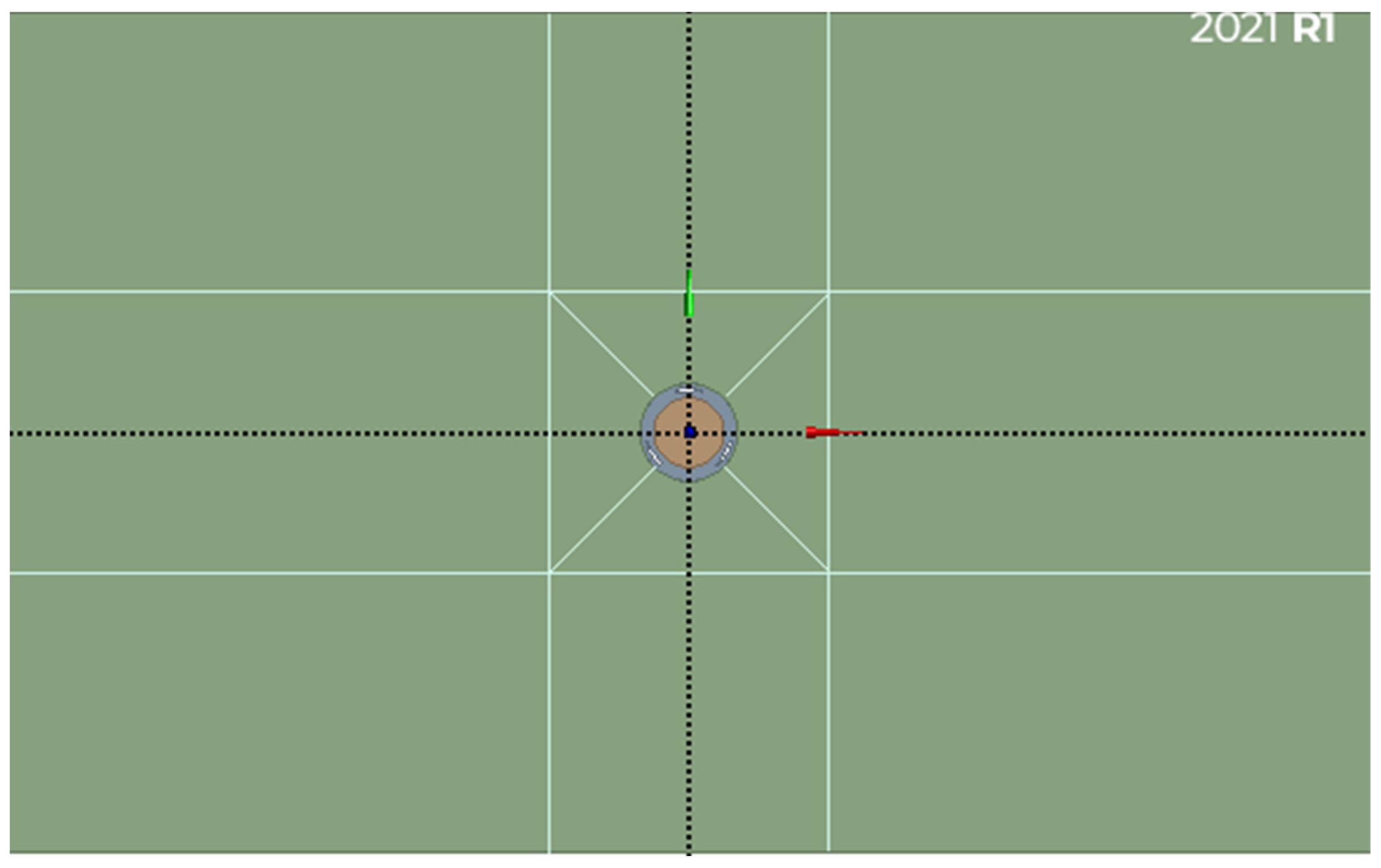
The first step in preparing the simulations was to create the geometry of the model. This was done using DesignModeler in Ansys Workbench. A .dat file of the aerofoil coordinates was obtained from Airfoil Tools [2]; the coordinates were imported as a line, and a pattern was used to create the three blades of the VAWT. Three surfaces were created to contain the flow and aid in meshing: one for the domain containing the blades, one for the domain inside the turbine, and one for the domain surrounding the VAWT. This can be seen in Figure 2. The VAWT uses a chord length of 1 m, a diameter of 3 m, an aerofoil shape of NACA 7715, and 3 blades. The size of the outer surface was chosen so that the total height of the domain (30 m) was 10 times the diameter of the turbine and the total width (60 m) was 20 times the diameter. This is so that there is enough room for the flow to develop without being affected by walls and is the same total domain size as that used by Durkacz et al. [24] with a centred VAWT as opposed to one offset closer to the inlet. The surface containing the blades was made slightly larger than the blades to comfortably accommodate them, and the inner surface filled in the rest.
3.2. Meshing
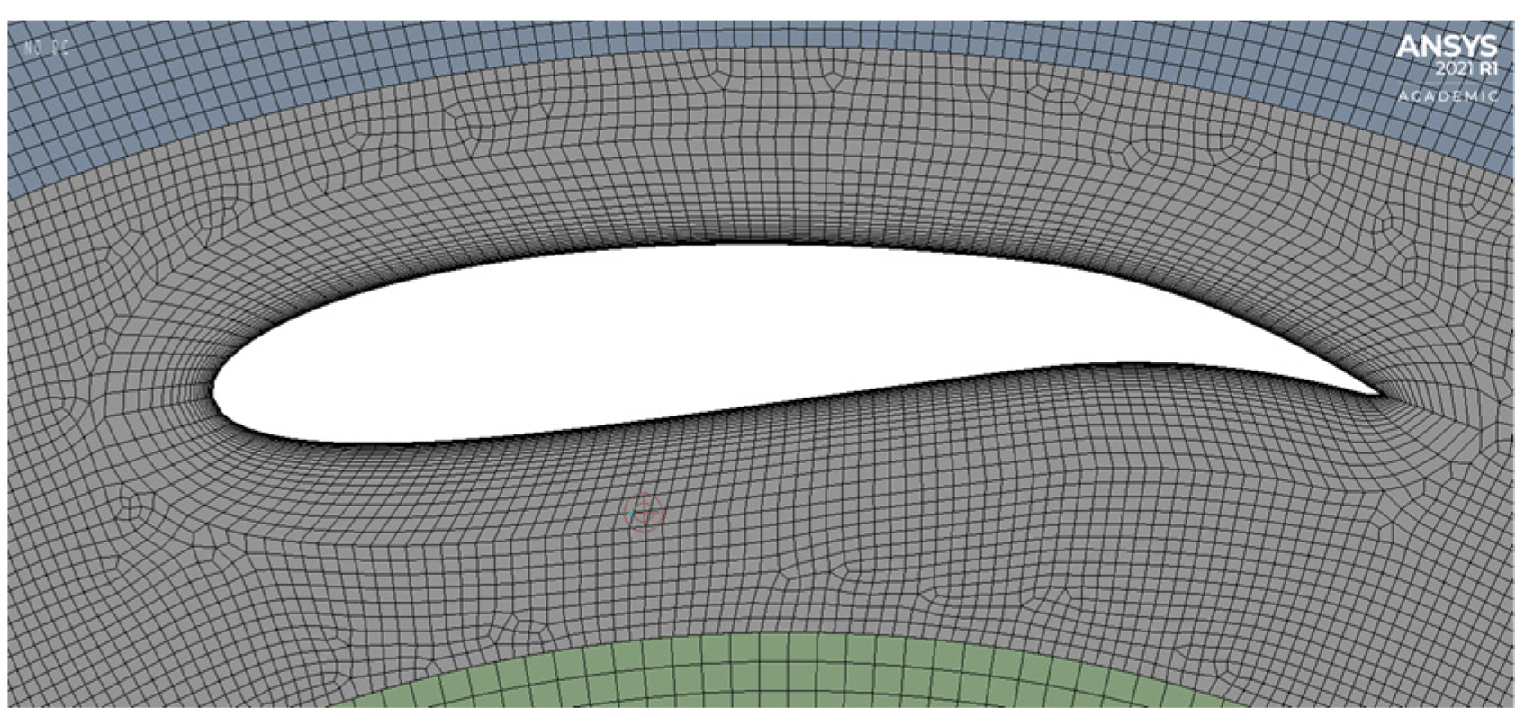
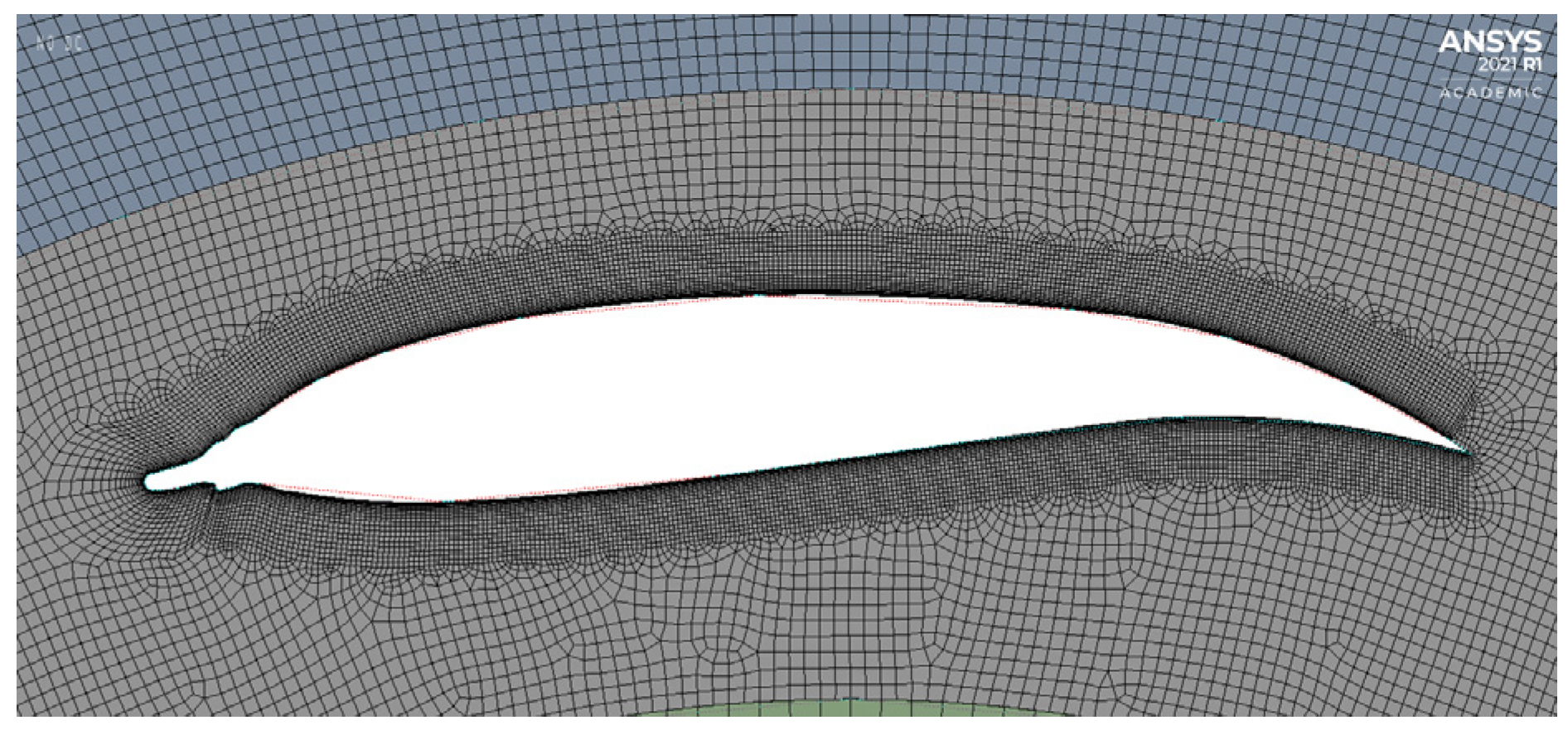
The geometry was imported into the meshing software within Ansys to create the mesh. This was done by applying a face sizing to each section and using sizing to create a denser mesh as it got close to the VAWT, with the densest section being the area containing the blades. This is because this area is expected to have the most variance in flow and is the main area of interest. An automatic method to create a quadrilateral dominant mesh was used on every surface, and inflation was also used around the blades to aid in capturing their complex shape. The mesh around the blade can be seen in Figure 3.
3.3. CFD Setup
The mesh was imported into Fluent to prepare for simulations. The settings used can be seen in Table 1. The SST k-ω viscous model was chosen based on the papers reviewed in Section 2.3. The turbulent intensity, turbulent length scale, and turbulent viscosity ratio were chosen based on values used by Lanzafame et al. [24] and Stout et al. [3]. Other values were tested, but the results did not differ enough to warrant changing them.
The solution was set up to output the moment coefficient as a file and a plot, so that the coefficient of performance can be calculated using the method shown in Section 2.1. Contours were also created to view the pressure and velocity around the VAWT, with animations being used to view contours at different points in the rotation. The simulations were set up to cover four full rotations of the VAWT in roughly 1200 time steps.
3.4. Clean Blade Simulations
To gain a better understanding of the VAWT being investigated, simulations were performed while changing the wind speed and chord length according to the values in Table 2. Simulations were also done to verify the mesh by varying the number of mesh elements and comparing that to the simulation time. Different simulation lengths and number of rotations were also investigated. Lastly, simulations were performed using the experimental dimensions for verification.
3.5. Obtaining Ice Shapes
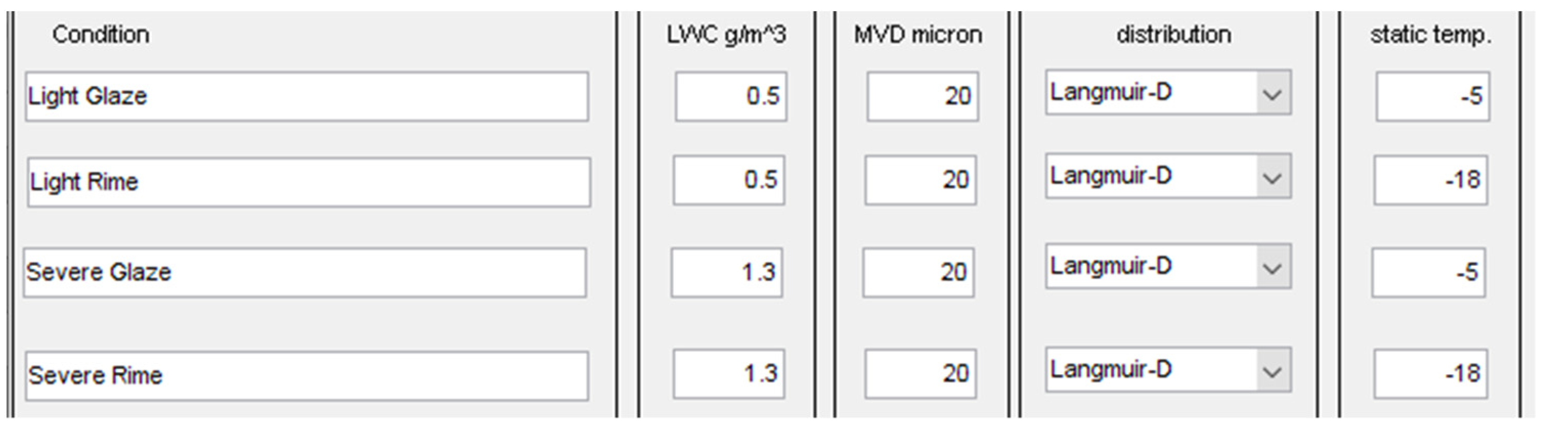
The ice shapes were obtained using LewInt, a free icing software that uses the LEWICE 3.2.2 ice accretion software code. To use the aerofoil shape as the geometry, the DAT file was converted into an XYD file. The chord length was set to the same as the simulations, and only the geometry of a single blade was used, as it was not possible to simulate rotation in the software. No thermal de-icer was applied, and the surface temperature of the blade was set to 273 K. The flight configuration and atmospheric configuration settings can be seen in Figure 4 and Figure 5, respectively. The velocity units are m/s, the altitude is in metres, and the temperature is in °C. The temperatures, LWCs, and median volume diameter (MVD) used were from categorisations made by EUMeTrain [5]. The velocity is the same as used in simulations, and the height is the average height above sea level of the UK. The altitude was varied, but very little change was observed. The times were determined based on observations made of the ice formations and any significant changes to the shapes. Verification was also performed using values used by Li [9] in icing wind tunnel experiments.
3.6. Ice Shape Simulations
The ice shapes were imported onto the geometry used in Section 3.4, with an additional edge sizing added around the blades to capture the ice shapes; see Figure 6. This was repeated for all eight ice shapes, and the results were compared to the clean blade results. The inflation had to be replaced with refinement for the mesh of the 3-h light glaze ice. Clean blade simulations were repeated with the adjusted mesh to verify it. The 5-h severe rime and glaze ice simulations were repeated at experimental scale.
3.7. Experiments
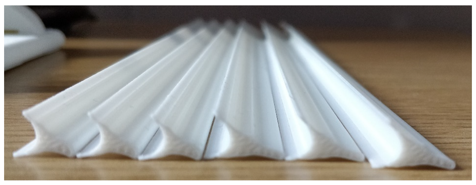
Two of the ice shapes were chosen and had their ice sections 3D printed. This was done by creating models in SolidWorks, exporting them as .stl files, then importing them into IdeaMaker to prepare for printing. The models were printed using PLA on a Raise 3D Pro 2 Plus 3D printer ( 3DGBIRE LTD, UK) and can be seen in Figure 7. Some of the shapes had errors at one of the ends, causing them to become rougher and contain small gaps. However, this was deemed to not be an issue, as the ice shapes were slightly longer than the blades they will be attached to.
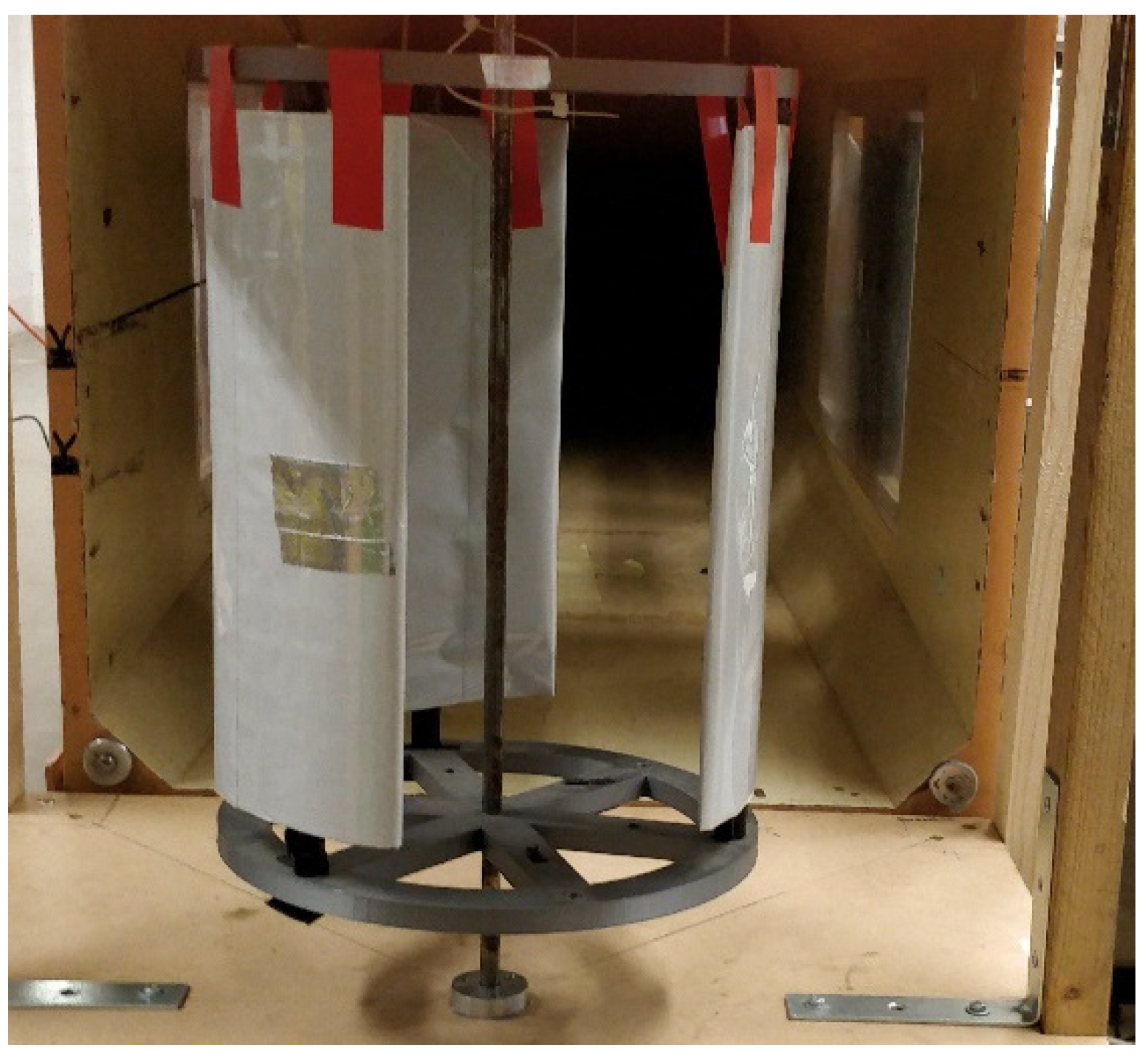
A wind tunnel was used to perform the experiments along with a scale VAWT model created by a previous student. The VAWT had a torque sensor build into it to measure the rpm, torque, and power generated. The torque sensor used was a Datum Electronics M425 Rotary Torque Sensor (Datum Electronics Ltd., East Cowes, UK), which connected to the computer through a PCB, where software was used to read the output. An anemometer was used to measure the wind speed of the tunnel, with speed being measured at the centre of the inlet and each corner before being averaged. The scale VAWT in front of the wind tunnel can be seen in Figure 8.
The experiments were repeated for two wind speeds and three different brake amounts. The brake amount refers to how tight the brakes on the top of the central axis of the VAWT were applied to create different TSRs. The same experiments were repeated with the ice shapes attached to the blades using tape.
4. Results: Clean Blade CFD
4.1. Mesh Analysis
The mesh analysis used five different mesh sizes for a four-rotation simulation. The time required to complete the simulation for each mesh can be seen in Table 3, with times for personal desktop and virtual desktop being recorded where possible. The coefficient of performance for each mesh was also calculated at five different TSRs. The percentage deviation from the previous mesh can be seen in Table 4.
From Table 4, it can be seen that the performance of the VAWT at the centre of the TSR range deviated by less than 5% between the last two meshes. There was more deviation at the outside of the TSR range, but the maximum performance occurs in the centre range, so it was deemed to be more important. Therefore, with the use of Table 3 and Table 4, it was determined that the 456k element mesh was sufficient to achieve accurate results in a reasonable time.
4.2. Simulation Time Analysis
A similar method to the mesh analysis was employed to determine the ideal simulation time. For this, the time step was kept constant, and the number of time steps was increased, making the VAWT complete more rotations. This was done for a range of 1–5 rotations, and it was found that the performance decreased as the number of rotations increased. A deviation of less than 5% was found between 4 rotations and 5 rotations, so 4 rotations were deemed to be suitably accurate. The time to complete the simulations scaled linearly with the number of rotations, so it was considered of less importance than the performance deviation.
4.3. Wind Speed Analysis
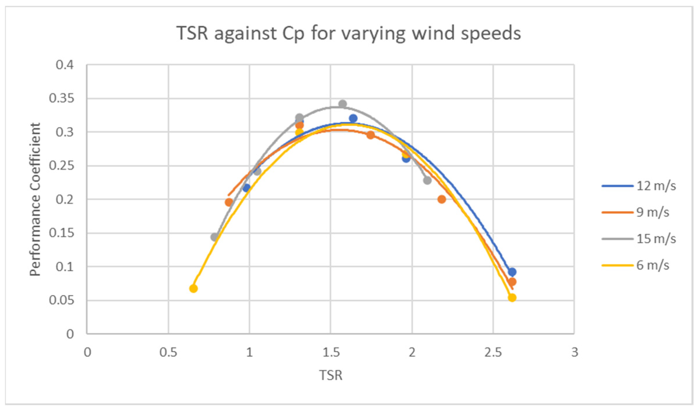
Simulations were performed at varying wind speeds to identify any changes in performance. The performance curves obtained can be seen in Figure 9.
The curves show that the performance does not vary much with wind speed, with the maximum performance occurring at around 1.5 TSR for each speed. The 15 m/s wind speed did show a slightly higher performance; however, a narrower range of TSRs was tested. Based on these data, it was decided that 12 m/s would be used for further simulations. The curves obtained were also found to agree with curves obtained by Durkacz et al. [4] and Li et al. [21].
4.4. Blade Scale Analysis
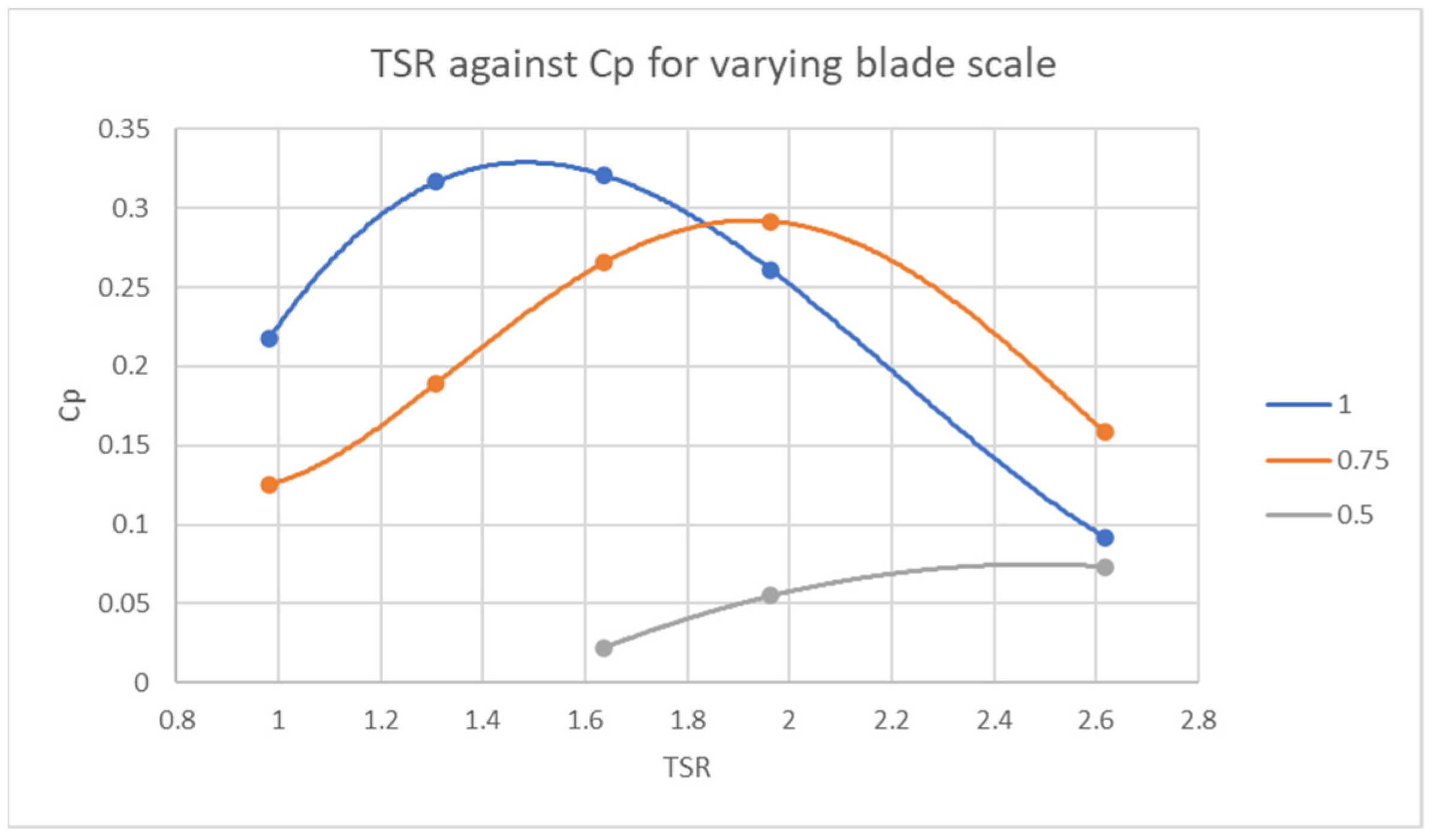
Simulations were also performed for different chord lengths by changing the scale of the blades. Scales of 1 and below were investigated to avoid getting too close to a cylinder. The performance curves can be seen in Figure 10. From the scales tested, the original scale showed the highest performance, with the 0.75 scale being close, but with the curve shifted to the right. Scales of 0.5 and 0.25 were also tested, but for the TSRs investigated, the performances found were mostly or all negative. Suggesting a scale of 0.5 or lower is not practical.
4.5. Velocity Contours
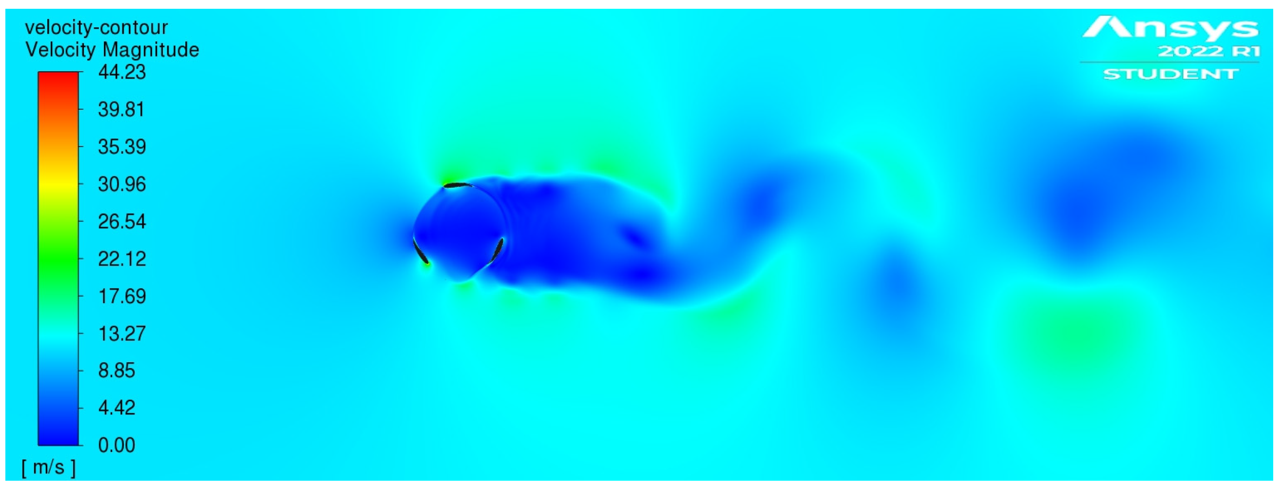
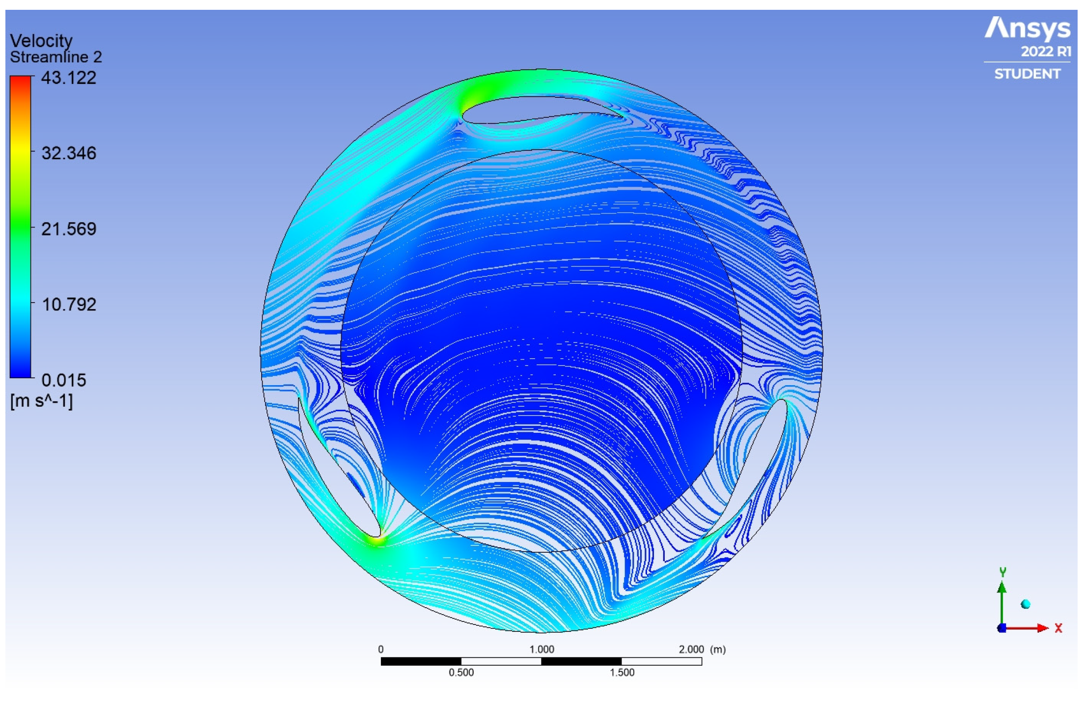
The velocity contour for one of the clean blade simulations can be seen in Figure 11. It shows that the wind loses almost all of its velocity when passing through the VAWT and for a distance after before it climbs back to the free stream velocity. The areas of higher velocity occurred at the surfaces of the blades. The streamlines inside the VAWT can be seen in Figure 12, and they show a recirculation of wind behind the bottom left blade and behind the trailing edge of the bottom right blade.
5. Results: Icing CFD
5.1. Ice Shapes
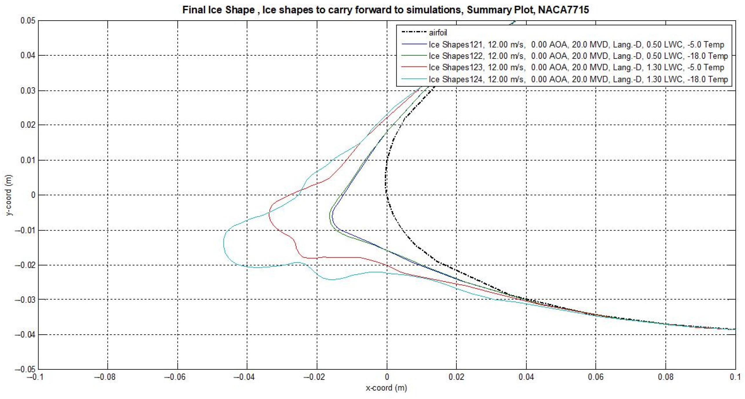
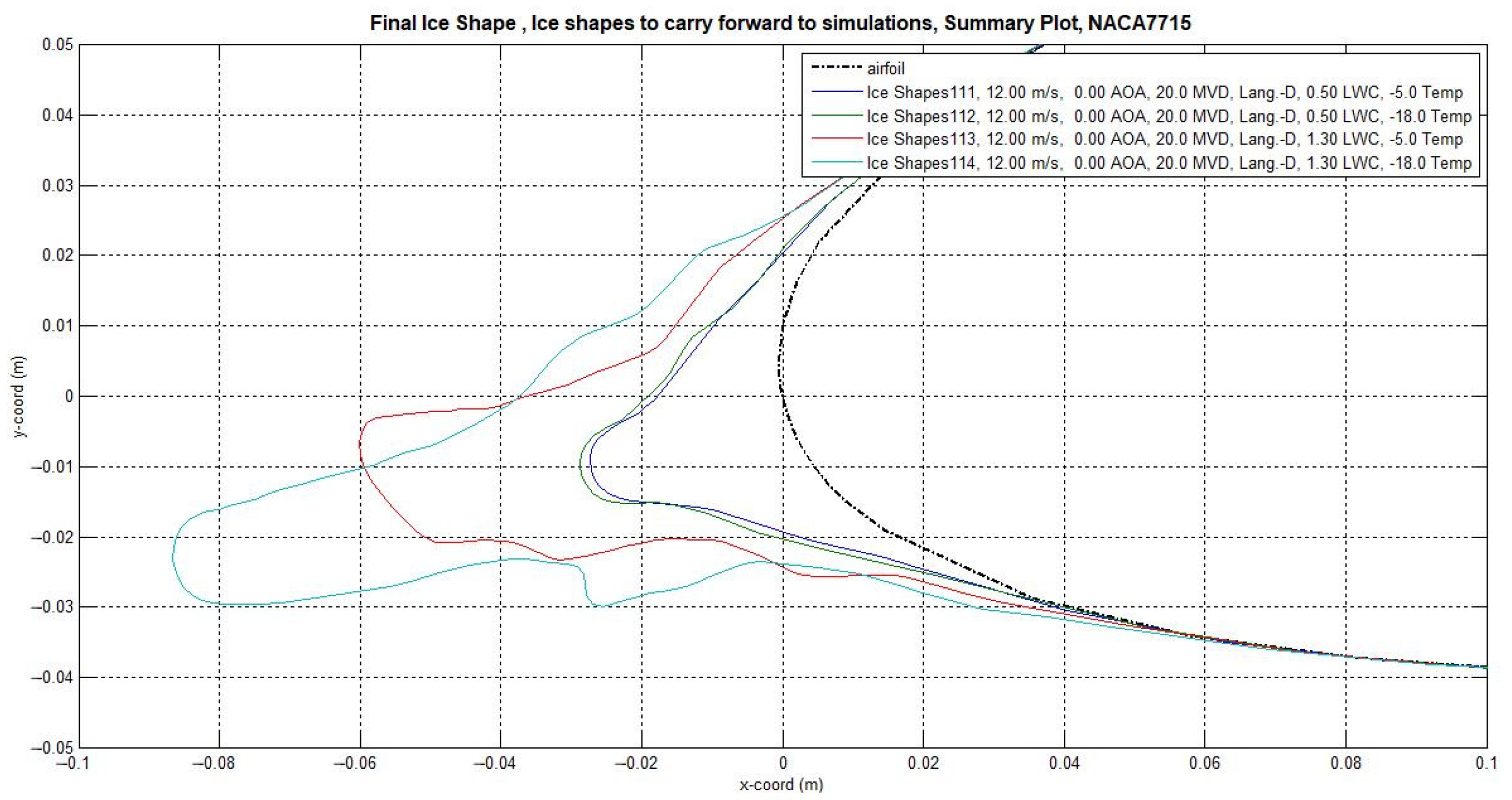
The ice shapes obtained from LewInt can be separated into 3-h and 5-h ice shapes. For each time, icing conditions that represented light and severe versions of rime and glaze ice were used. The obtained ice shapes can be seen in Figure 13 and Figure 14. The dashed line represents the clean blade; dark blue is light rime; green is light glaze; red is severe rime; and cyan is severe glaze. Only the leading edge is shown, as ice did not form anywhere else.
The light rime and light glaze ice shapes formed a rounded point at the leading edge, with a slight protrusion appearing in the 5-h shapes. Rime and glaze ice showed little difference in light conditions. The severe conditions showed much larger ice shapes, with glaze ice creating a larger horn at the leading edge than the rime ice. There was also a noticeable size difference between the 3-h and 5-h ice shapes, suggesting that time makes a larger difference in severe conditions than in light conditions.
Verification was performed by obtaining ice shapes using the same conditions as Li et al. [9] in their icing experiment. A comparison of two of the shapes can be seen in Figure 15. The shapes agreed on the general shape of ice formation at the leading edge, with the simulation being smoother. However, the simulation was unable to capture the ice formation on the trailing edge that was found in the experiments. Verification of ice shapes performed at different times agreed with the increase of ice thickness with time.
5.2. Performance Simulations
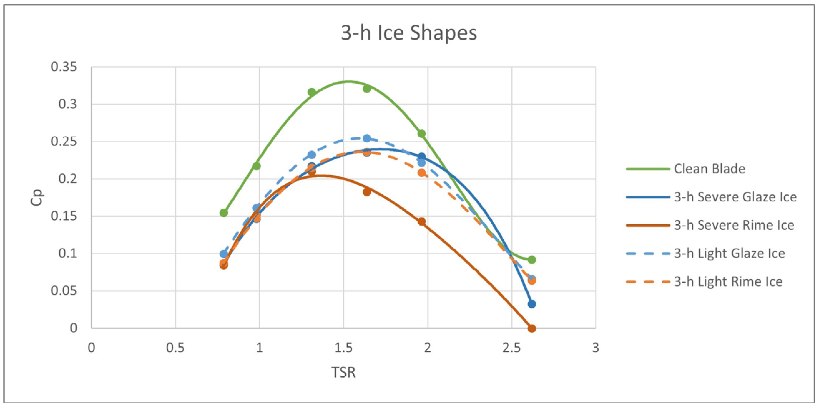
The performance curves obtained for the 3-h ice shapes and the 5-h ice shapes can be seen in Figure 16 and Figure 17, respectively. Both graphs contain the clean blade performance curve for the same wind speed as a comparison. It can be seen from the figures that all of the ice shapes had a significant effect on the performance of the VAWT, with a minimum peak power reduction of 20% occurring with the 3-h light glaze ice. The largest decrease in power was found in the 5-h severe rime ice conditions, with a decrease of 40%. Increasing from 3 h of icing time to 5 h caused a decrease in performance at every TSR for most shapes tested.
The 3-h light glaze ice used an unstructured mesh when all of the others used a structured mesh. The unstructured mesh was used to avoid errors where the moment coefficient would spike to unrealistic values when performing simulations with the structured mesh. Simulations performed using this mesh on the clean blade showed that the unstructured mesh overpredicts the performance of the VAWT. Therefore, the 3-h light glaze ice curve in Figure 16 is likely an overprediction. However, comparing the 3-h and 5-h performance curves suggests that the light glaze ice and light rime ice curves should be similar.
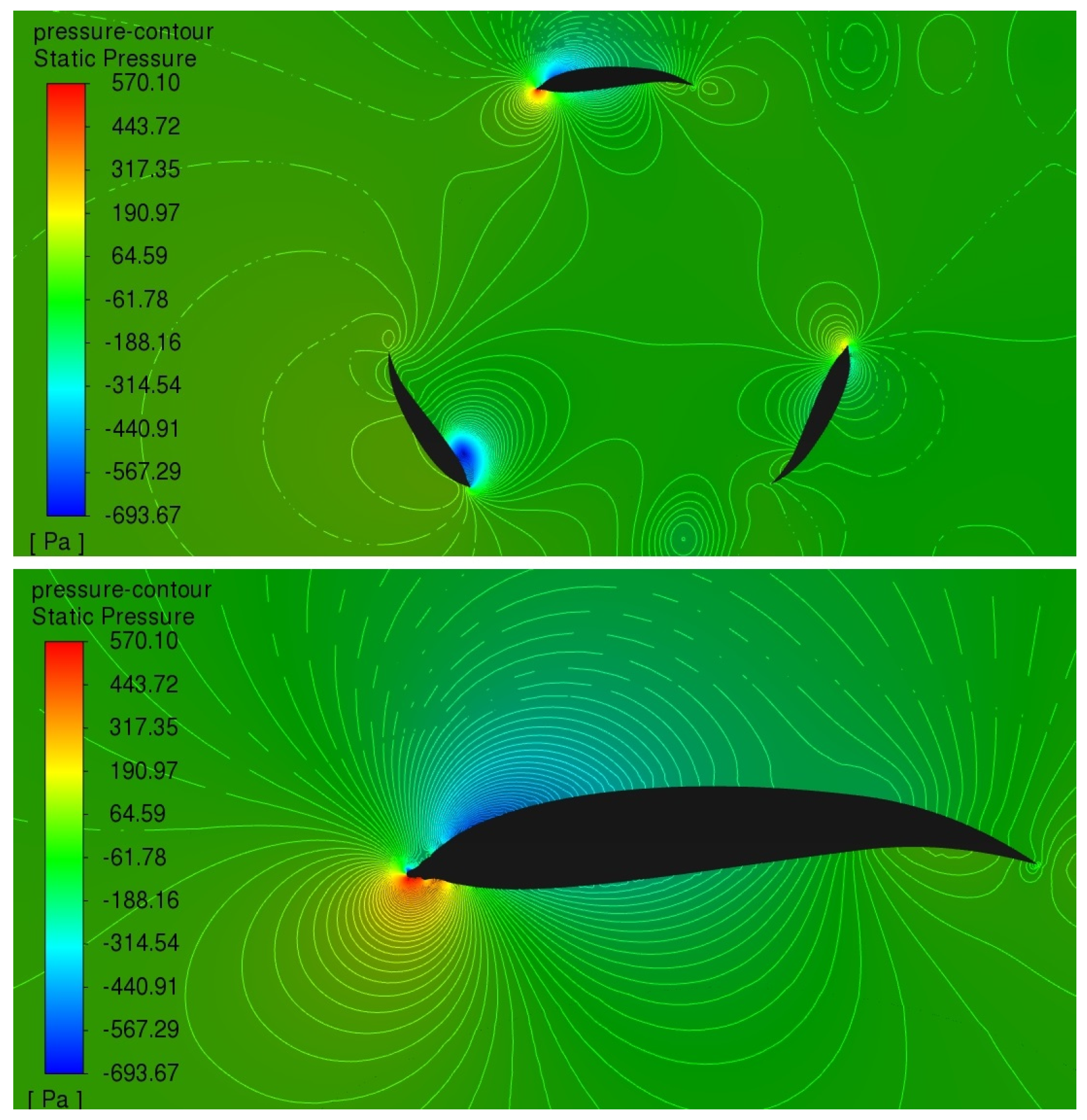
5.3. Pressure Contours
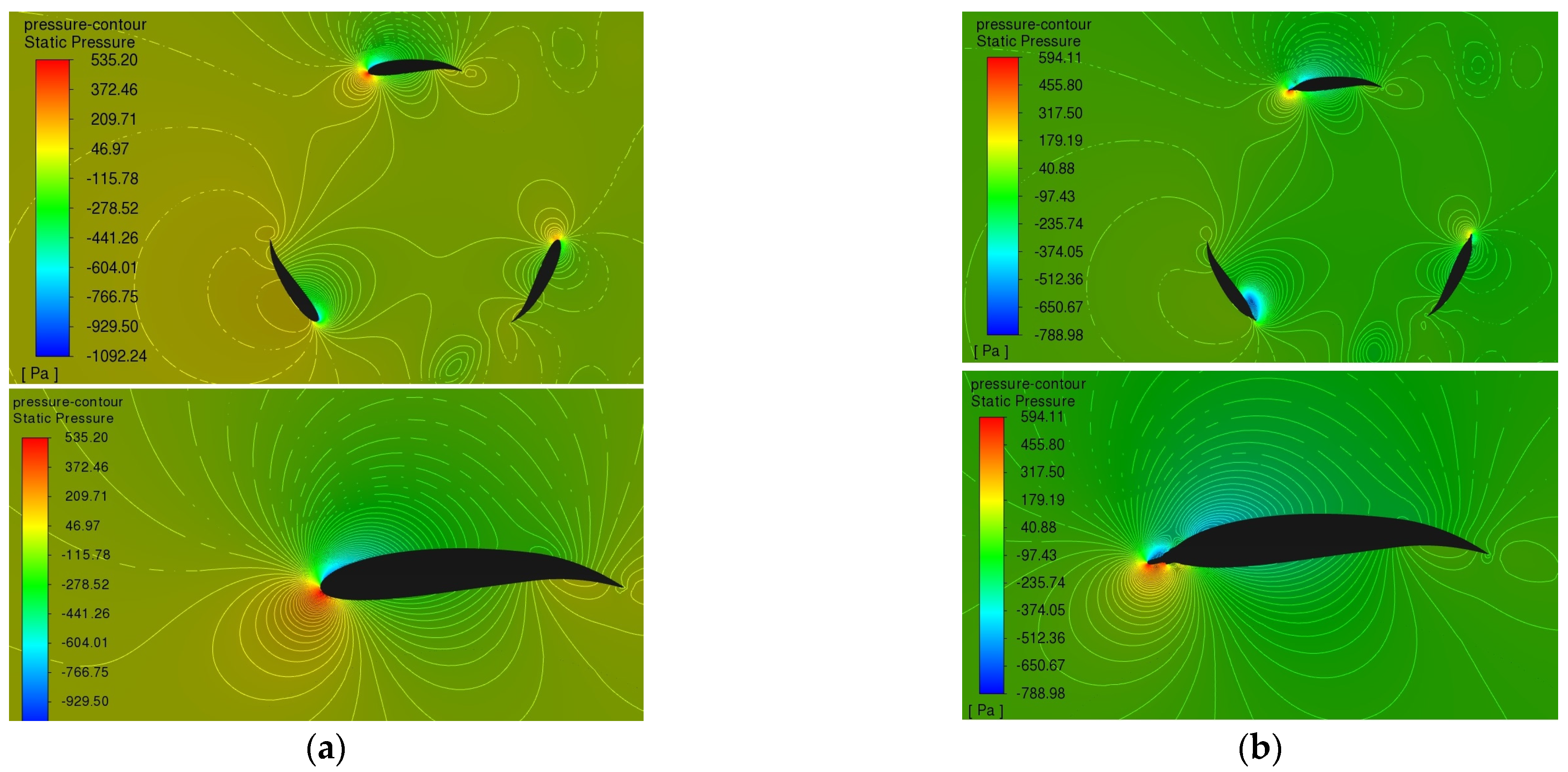
To help explain the decrease in performance, pressure contours for the clean blade VAWT and the most severe ice shape, the 5-h severe rime ice, were created. These can be seen in Figure 18. The contours show that the maximum pressure was greater in the icing example, with a maximum of 594 Pa compared to the 535 Pa maximum in the clean blade. However, the clean blade produced a larger negative pressure of −1009 Pa compared to the −789 Pa of the icing example. The largest positive and negative values of pressure occurred at the leading edges of the blades, as can be seen in the close-ups. These close-ups also show that the icing moves the area of high positive pressure away from the original aerofoil shape and to the tip of the lower edge of the ice formation. The same can be seen for the area of high negative pressure on the top of the ice shape. The ice shape also causes a second area of high negative pressure to form along the top of the aerofoil just behind the tip.
The pressure contours for the 3-h severe rime ice were also investigated and can be seen in Figure 19. This shows that the areas of high and low pressure remain in a similar position between icing conditions, with the 3-h severe rime ice not having a pronounced secondary area of high negative pressure. The 3-h severe rime ice also caused a smaller maximum and minimum pressure than the 5-h, with a maximum of 570 Pa and a minimum of −694 Pa.
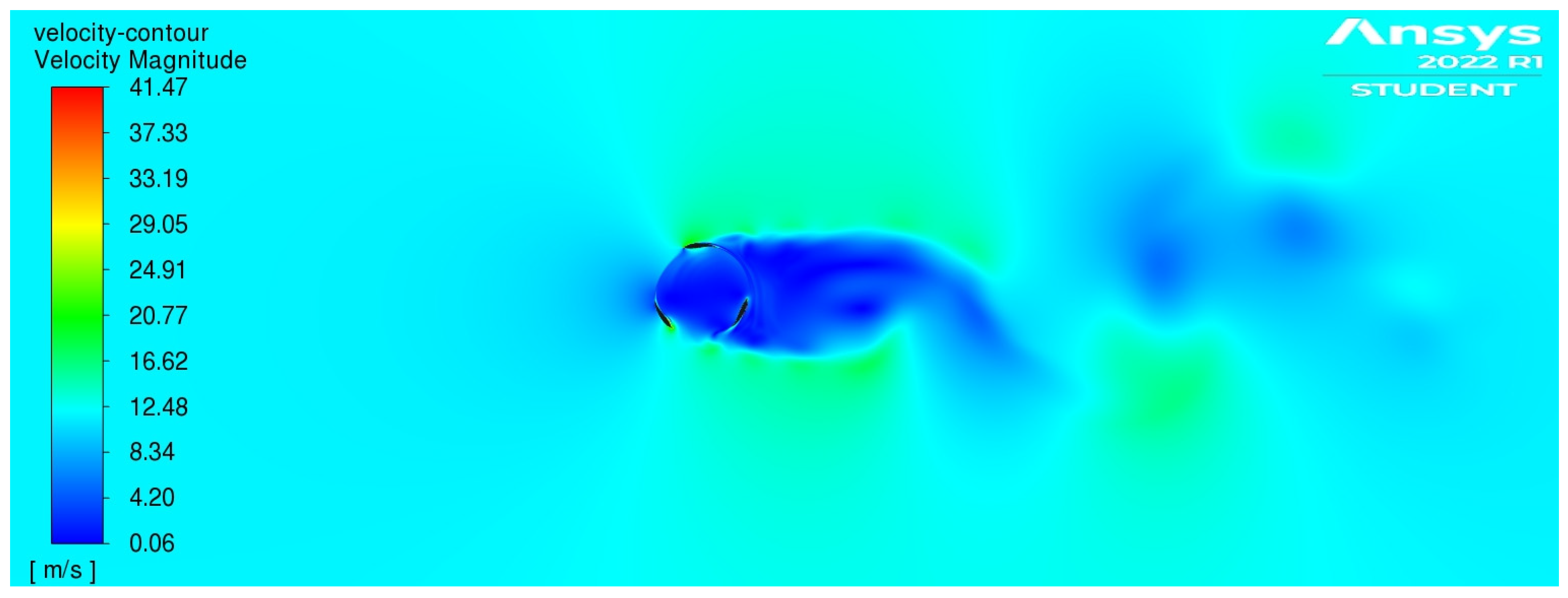
5.4. Velocity Contour
The velocity contour for the 5-h severe rime ice, see Figure 20, was investigated to see if there were any notable changes from the contour for the clean blade VAWT in Figure 11. It showed a similar velocity to the clean blade, with the notable differences being larger areas of high velocity around the blades and the velocity after leaving the turbine regenerating in a different manner. The maximum velocity was found to have decreased from the 44.2 m/s of the clean blade to 41.5 m/s.
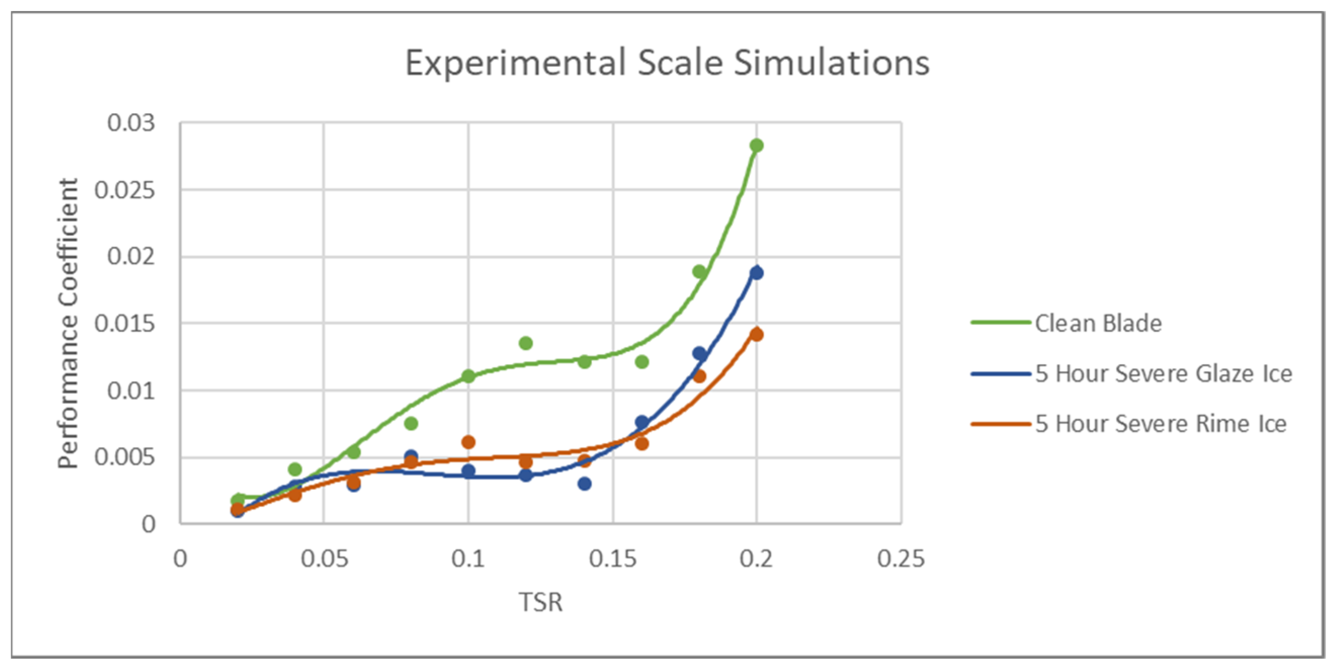
5.5. Scale Simulations
Scale simulations were performed to compare with experimental results for the 5-h severe rime and glaze ice. The performance curves can be seen in Figure 21. The simulations focused on low TSRs, as the TSRs used in the experiment are expected to be low due to a smaller radius and assuming a reasonable rotational speed. These curves showed a similar decrease in performance to that found in the full TSR range.
6. Results: Experiments
6.1. Clean Blade Experiment
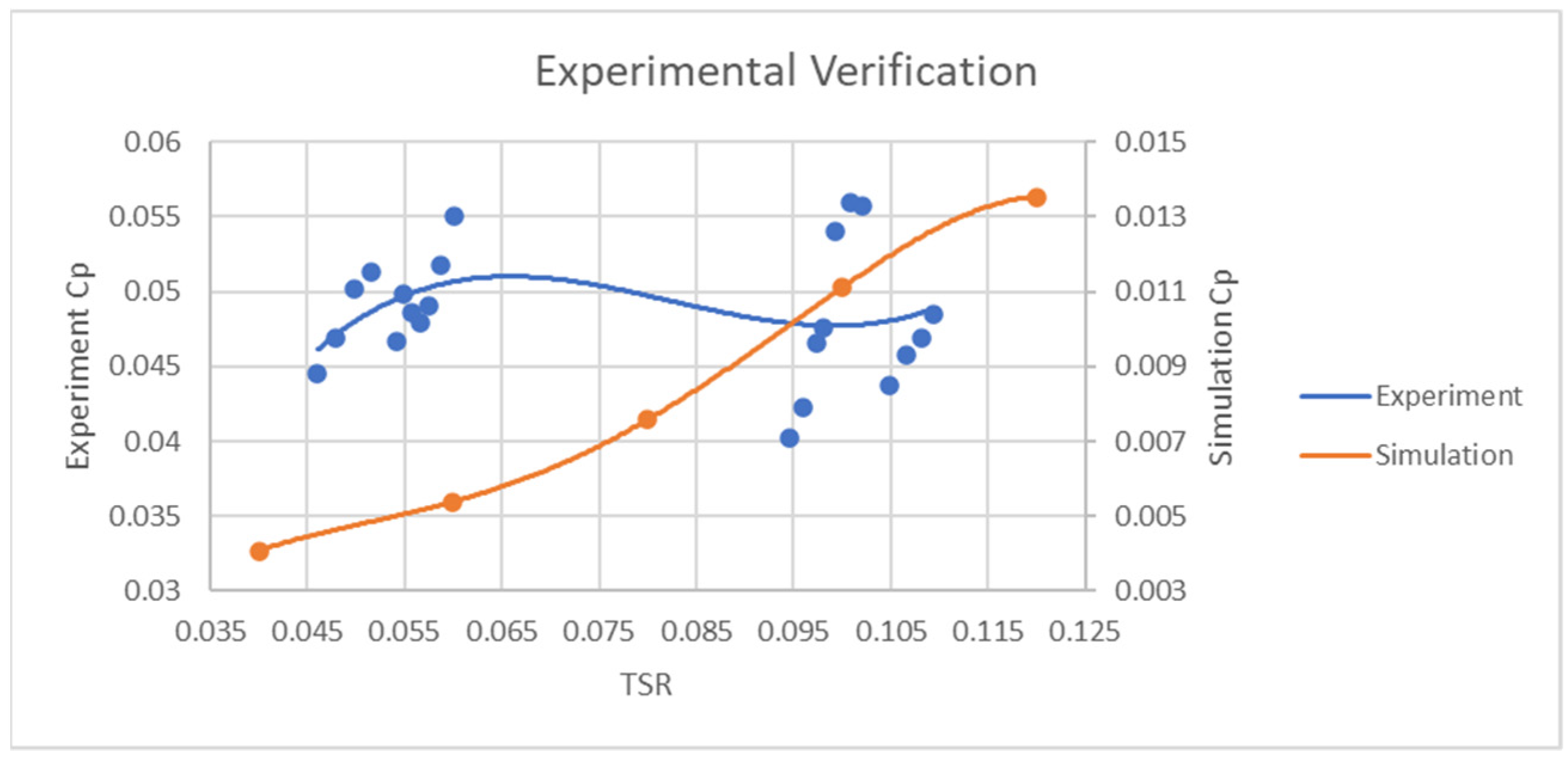
The performance curve obtained from the experiment can be seen in Figure 22 alongside the curve from the scale simulation. The results obtained from the experiment were separated into similar TSRs and averaged to reduce the spread of the results. The spread of the data caused a mostly flat trend line to occur, suggesting that the performance of the VAWT did not change much in the TSR range, whereas the simulation predicted a gradual increase in performance. This is likely caused by an assumption in the simulation but could also be caused the spread of experimental results, with more results at different TSRs changing the curve. The performance from the experiment was also much greater than the simulations, at around 4–10 times the performance at different TSRs. Additional verification using this experimental model was performed by Durkacz et al. [4], where the performance at a 12 m/s wind speed was compared for experimental and two differing simulation methods. Durkacz et al. [4] found a linear increase in performance with TSR for each method over the TSR range of 0.03–0.07, suggesting that with more data, a similar trend would be seen in the current experimental work. Durkacz et al. [4] also found that the experimental values for performance were much greater than those found in the simulations.
6.2. Icing Experiments
The same experiments were repeated using the 5-h severe rime and glaze ice shapes attached to the VAWT. When performing the experiments, a sustained rotation of the model was not able to be obtained for any amount of braking or wind speed possible with the wind tunnel, so no numerical results were able to be obtained. However, this suggests that these ice shapes cause a severe reduction in performance on a small scale, preventing the VAWT from generating any power. This agrees with the power reduction found in the simulations and suggests that the simulations may not be able to convey the impact of the ice on the ability of the VAWT to sustain rotation.
7. Conclusions & Recommendations
7.1. Conclusions
Work was performed to gain a better insight into how the formation of ice affects the aerodynamics and performance of a VAWT, along with an understanding of the current performance of the VAWT. From this work, the following conclusions were drawn:
- Altering the wind speed only caused minor changes to the performance of the clean blade VAWT, with the performance increasing slightly with higher wind speeds.
- Reducing the scale of the blade significantly decreased the performance of the clean blade VAWT, with a scale of 1 providing the best performance.
- Increasing the icing time led to the ice thickness increasing, with a horn shape forming in severe cases that protruded further with time.
- The LWC and MVD severely affected the formation of ice. Lighter conditions caused thinner ice shapes with no notable protrusions, whereas severe conditions caused thicker ice shapes with notable protrusions.
- Rime icing conditions led to the formation of larger ice shapes compared to glaze ice.
- All the icing conditions caused a significant decrease in performance, with a maximum of 40% in the 5-h severe rime ice case.
- The ice shapes moved the areas of high and low pressure off the aerofoil and onto the tip of the ice shape, with a secondary area of low pressure found in one case.
- Experimental tests showed an even more severe reduction in performance with icing, as the scale models could not sustain rotation with the ice shapes attached.
7.2. Recommendations
It is recommended that for VAWTs being installed in climates likely to cause icing, action be taken to prevent significant losses. This could be done by installing anti-icing or de-icing features such as those investigated by Wei et al. [19]. For further work on investigating the impact of ice formation on the performance of a VAWT or to continue this work, the following steps are recommended:
- Perform experiments using a VAWT closer to the scale of the actual VAWT to get a better understanding of how a full-size VAWT would perform and to identify and reduce any inaccuracies caused by scaling.
- To avoid a similar situation where numerical results could not be obtained from the experimental tests using the ice shapes, it is recommended that the following be considered: use a wind tunnel with a higher maximum speed, use smaller ice shapes to reduce their impact on performance, or use an alternative method to create and attach the ice shapes.
- Perform 3D simulations to get a more accurate representation of the impact for an actual VAWT by considering how ice would form at the ends of the blades and how this would impact performance along with other factors such as proximity of the VAWT to the ground.
- Investigate the formation of ice on the trailing edge of the blade and its effect on the performance when combined with the formation on the leading edge. This could potentially be done by using a Eulerian approach as opposed to a Lagrangian approach when simulating the ice formation.
- Investigate the use of anti-icing and de-icing techniques and how much performance can be recovered using these techniques.
Author Contributions
Conceptualization, S.G., S.Z.I. and T.A.; methodology, S.G.; software, S.G.; validation, S.G.; formal analysis, S.G.; investigation, S.G., C.G. and S.Z.I.; resources, S.G.; data curation, S.G.; writing—original draft preparation, S.G.; writing—review and editing, S.G, S.Z.I. and G.D.; visualization, S.G.; supervision, S.Z.I.; project administration, S.G and S.Z.I. All authors have read and agreed to the published version of the manuscript.
Funding
This research received no external funding.
Institutional Review Board Statement
Not applicable.
Informed Consent Statement
Not applicable.
Data Availability Statement
The data that support the findings of this study are available from the corresponding author at [email protected] upon reasonable request.
Acknowledgments
The authors are grateful to the School of Engineering, Robert Gordon University, United Kingdom, for supporting this research. The technical staff at RGU for their assistance with 3D printing and the wind tunnel experiments.
Conflicts of Interest
The authors declare no conflict of interest.
References
- Available online: https://www.gov.scot/binaries/content/documents/govscot/publications/statistics/2018/10/quarterly-energy-statistics-bulletins/documents/energy-statistics-summary---march-2021/energy-statistics-summary---march-2021/govscot:document/Scotland+Energy+Statistics+Q4+2020.pdf (accessed on 18 February 2022).
- NACA 4 Digit Airfoil Generator. Available online: http://airfoiltools.com/airfoil/naca4digit (accessed on 5 March 2022).
- Stout, C.; Islam, S.; White, A.; Arnott, S.; Kollovozi, E.; Shaw, M.; Droubi, G.; Sinha, Y.; Bird, B. Efficiency Improvement of Vertical Axis Wind Turbines with an Upstream Deflector. Energy Procedia 2017, 118, 141–148. [Google Scholar] [CrossRef]
- Durkacz, J.; Islam, S.; Chan, R.; Fong, E.; Gillies, H.; Karnik, A.; Mullan, T. CFD modelling and prototype testing of a Vertical Axis Wind Turbines in planetary cluster formation. Energy Rep. 2021, 7, 119–126. [Google Scholar] [CrossRef]
- Icing. Available online: http://www.eumetrain.org/data/2/253/print_2.htm (accessed on 25 February 2022).
- Guo, W.; Shen, H.; Li, Y.; Feng, F.; Tagawa, K. Wind tunnel tests of the rime icing characteristics of a straight-bladed vertical axis wind turbine. Renew. Energy 2021, 179, 116–132. [Google Scholar] [CrossRef]
- Li, Y.; Wang, S.; Liu, Q.; Feng, F.; Tagawa, K. Characteristics of ice accretions on blade of the straight-bladed vertical axis wind turbine rotating at low tip speed ratio. Cold Reg. Sci. Technol. 2018, 145, 1–13. [Google Scholar] [CrossRef]
- Li, Y.; Tagawa, K.; Feng, F.; Li, Q.; He, Q. A wind tunnel experimental study of icing on wind turbine blade airfoil. Energy Convers. Manag. 2014, 85, 591–595. [Google Scholar] [CrossRef]
- Li, Y.; Tang, J.; Liu, Q.D.; Wang, S.L.; Feng, F. A visualization experimental study of icing on blade for VAWT by wind tunnel test. In Advances in Engineering Research, Proceedings of the 2015 International Conference on Power Electronics and Energy Engineering; Atlantis Press: Amsterdam, The Netherlands, 2015; p. 147. [Google Scholar]
- Hann, R.; Hearst, R.J.; Sætran, L.R.; Bracchi, T. Experimental and Numerical Icing Penalties of an S826 Airfoil at Low Reynolds Numbers. Aerospace 2020, 7, 46. [Google Scholar] [CrossRef] [Green Version]
- Yan, L.; Yuan, C.; Yongjun, H.; Shengmao, L.; Kotaro, T. Numerical simulation of icing effects on static flow field around blade airfoil for vertical axis wind turbine. Int. J. Agric. Biol. Eng. 2011, 4, 41–47. [Google Scholar]
- Villalpando, F.; Reggio, M.; Ilinca, A. Prediction of ice accretion and anti-icing heating power on wind turbine blades using standard commercial software. Energy 2016, 114, 1041–1052. [Google Scholar] [CrossRef]
- Shin, J.; Berkowitz, B.; Chen, H.H.; Cebeci, T. Prediction of ice shapes and their effect on airfoil drag. J. Aircr. 1994, 31, 263–270. [Google Scholar] [CrossRef]
- Manatbayev, R.; Baizhuma, Z.; Bolegenova, S.; Georgiev, A. Numerical simulations on static Vertical Axis Wind Turbine blade icing. Renew. Energy 2021, 170, 997–1007. [Google Scholar] [CrossRef]
- Baizhuma, Z.; Kim, T.; Son, C. Numerical method to predict ice accretion shapes and performance penalties for rotating vertical axis wind turbines under icing conditions. J. Wind Eng. Ind. Aerodyn. 2021, 216, 104708. [Google Scholar] [CrossRef]
- Martini, F.; Contreras Montoya, L.T.; Ilinca, A. Review of Wind Turbine Icing Modelling Approaches. Energies 2021, 14, 5207. [Google Scholar] [CrossRef]
- Ibrahim, G.M.; Pope, K.; Muzychka, Y.S. Effects of blade design on ice accretion for horizontal axis wind turbines. J. Wind Eng. Ind. Aerodyn. 2018, 173, 39–52. [Google Scholar] [CrossRef]
- Wei, K.; Yang, Y.; Zuo, H.; Zhong, D. A review on ice detection technology and ice elimination technology for wind turbine. Wind Energy 2020, 23, 433–457. [Google Scholar] [CrossRef]
- Drapalik, M.; Zajicek, L.; Purker, S. Ice aggregation and ice throw from small wind turbines. Cold Reg. Sci. Technol. 2021, 192, 103399. [Google Scholar] [CrossRef]
- Barber, S.; Wang, Y.; Jafari, S.; Chokani, N.; Abhari, R.S. The impact of ice formation on wind turbine performance and aerodynamics. Sol. Energy Eng. 2011, 133, 011007. [Google Scholar] [CrossRef]
- Li, Q.; Maeda, T.; Kamada, Y.; Murata, J.; Kawabata, T.; Shimizu, K.; Ogasawara, T.; Nakai, A.; Kasuya, T. Wind tunnel and numerical study of a straight-bladed Vertical Axis Wind Turbine in three-dimensional analysis (Part II: For predicting flow field and performance). Energy 2016, 104, 295–307. [Google Scholar] [CrossRef]
- Fu, P.; Farzaneh, M. A CFD approach for modeling the rime-ice accretion process on a horizontal-axis wind turbine. J. Wind Eng. Ind. Aerodyn. 2010, 98, 181–188. [Google Scholar] [CrossRef]
- Hu, L.; Zhu, X.; Chen, J.; Shen, X.; Du, Z. Numerical simulation of rime ice on NREL Phase VI blade. J. Wind. Eng. Ind. Aerodyn. 2018, 178, 57–68. [Google Scholar] [CrossRef]
- Lanzafame, R.; Mauro, S.; Messina, M. 2D CFD Modeling of H-Darrieus Wind Turbines Using a Transition Turbulence Model. Energy Procedia 2014, 45, 131–140. [Google Scholar] [CrossRef] [Green Version]
Figure 1.
NACA 7715 aerofoil (1 m chord length) [2].
Figure 1.
NACA 7715 aerofoil (1 m chord length) [2].

Figure 2.
DesignModeler geometry.

Figure 3.
Mesh around a blade.

Figure 4.
LewInt flight configuration.

Figure 5.
LewInt atmospheric configuration.

Figure 6.
Mesh around the 5-h severe rime ice blade.

Figure 7.
3D printed ice shapes.

Figure 8.
Vertical axis wind turbine (VAWT) in front of the wind tunnel.

Figure 9.
Performance curve for varying wind speeds.

Figure 10.
Performance curve for varying blade scales.

Figure 11.
Clean blade velocity contour (12 m/s, 1.6 TSR).

Figure 12.
Velocity streamlines inside the clean blade VAWT (12 m/s, 1.6 TSR).

Figure 13.
3-h ice shapes obtained using LewInt.

Figure 14.
5-h ice shapes obtained using LewInt.

Figure 15.
Comparison of ice shapes obtained after 19 min: (a) Experimental shapes obtained by Li et al. [9]; (b) Shape obtained through LewInt.
Figure 15.
Comparison of ice shapes obtained after 19 min: (a) Experimental shapes obtained by Li et al. [9]; (b) Shape obtained through LewInt.

Figure 16.
3-h ice shape performance curves.

Figure 17.
5-h ice shape performance curves.

Figure 18.
Pressure contours for full VAWT and blade close-up (12 m/s, 1.6 TSR): (a) Clean blade; (b) 5-h severe rime ice.
Figure 18.
Pressure contours for full VAWT and blade close-up (12 m/s, 1.6 TSR): (a) Clean blade; (b) 5-h severe rime ice.

Figure 19.
3-h severe rime ice contour for full VAWT and blade close-up (12 m/s, 1.6 TSR).

Figure 20.
5-h severe rime ice velocity contour (12 m/s, 1.6 TSR).

Figure 21.
Experimental scale performance curves.

Figure 22.
Clean blade experiment performance curve.


Table 1.
Computation fluid dynamics (CFD) setup parameters.
| Time | Transient |
|---|---|
| Viscous Model | SST k-ω |
| Fluid | Air |
| Reference Area [m2] | 3 |
| Reference Depth [m] | 1 |
| Reference Length [m] | 1.5 |
| Reference Velocity [m/s] | Same as inlet velocity |
| Inlet X-Velocity [m/s] | 6, 9, 12, 15 |
| Inlet Turbulent Intensity [%] | 2 |
| Inlet Turbulent Length Scale [m] | 1 |
| Outlet Gauge Pressure [Pa] | 0 |
| Backflow Turbulent Intensity [%] | 2.2 |
| Backflow Turbulent Viscosity Ratio | 0.1 |
Table 2.
Wind speed and chord lengths investigated.
| Simulation Parameter | Values |
|---|---|
| Wind Speed (m/s) | 6, 9, 12, 15 |
| Chord Length (m) | 0.25, 0.5, 0.75, 1 |
Table 3.
Mesh analysis simulation times (personal desktop/virtual desktop).
| Mesh Elements | Time for 4 Rotations (min) |
|---|---|
| 112,752 | 68/103 |
| 234,096 | 113/188 |
| 324,311 | 156/- |
| 456,160 | 212/- |
| 580,706 | -/331 |
Table 4.
Percentage deviation from the previous mesh of coefficient of performance.
| TSR | 112,757 | 234,096 | 324,311 | 465,160 | 580,706 |
|---|---|---|---|---|---|
| 0.982 | 0% | 44.3% | 15.0% | 6.6% | 5.1% |
| 1.309 | 0% | 54.4% | 17.8% | 7.3% | 3.5% |
| 1.636 | 0% | 52.7% | 11.1% | 4.3% | 0.2% |
| 1.963 | 0% | 164.6% | 13.0% | 5.2% | −1.4% |
| 2.618 | 0% | 0% | 49.1% | 5.7% | −15.5% |
Disclaimer/Publisher’s Note: The statements, opinions and data contained in all publications are solely those of the individual author(s) and contributor(s) and not of MDPI and/or the editor(s). MDPI and/or the editor(s) disclaim responsibility for any injury to people or property resulting from any ideas, methods, instructions or products referred to in the content. |
© 2023 by the authors. Licensee MDPI, Basel, Switzerland. This article is an open access article distributed under the terms and conditions of the Creative Commons Attribution (CC BY) license (https://creativecommons.org/licenses/by/4.0/).
Share and Cite
MDPI and ACS Style
Gerrie, S.; Islam, S.Z.; Gerrie, C.; Droubi, G.; Asim, T. The Impact of Ice Formation on Vertical Axis Wind Turbine Performance and Aerodynamics. Wind 2023, 3, 16-34. https://doi.org/10.3390/wind3010003
AMA Style
Gerrie S, Islam SZ, Gerrie C, Droubi G, Asim T. The Impact of Ice Formation on Vertical Axis Wind Turbine Performance and Aerodynamics. Wind. 2023; 3(1):16-34. https://doi.org/10.3390/wind3010003
Chicago/Turabian StyleGerrie, Sean, Sheikh Zahidul Islam, Cameron Gerrie, Ghazi Droubi, and Taimoor Asim. 2023. "The Impact of Ice Formation on Vertical Axis Wind Turbine Performance and Aerodynamics" Wind 3, no. 1: 16-34. https://doi.org/10.3390/wind3010003