
Cascaded H-Bridge Multilevel Converter Applied to a Wind Energy Conversion System with Open-End Winding
 , , and
Abstract
:1. Introduction
2. System Description
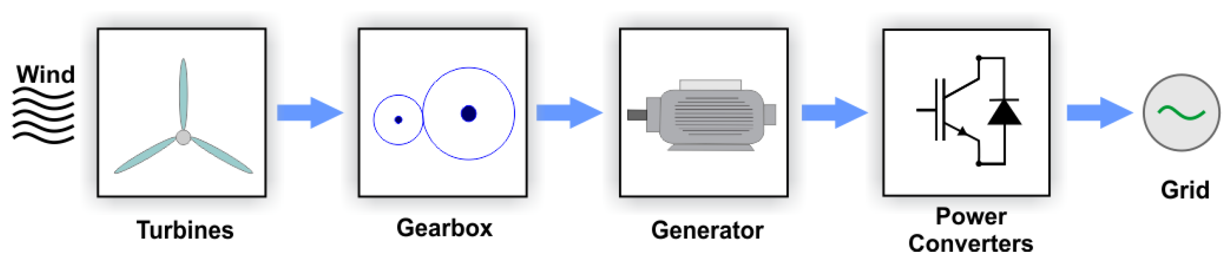
2.1. Wind Energy Conversion System
2.2. Generator
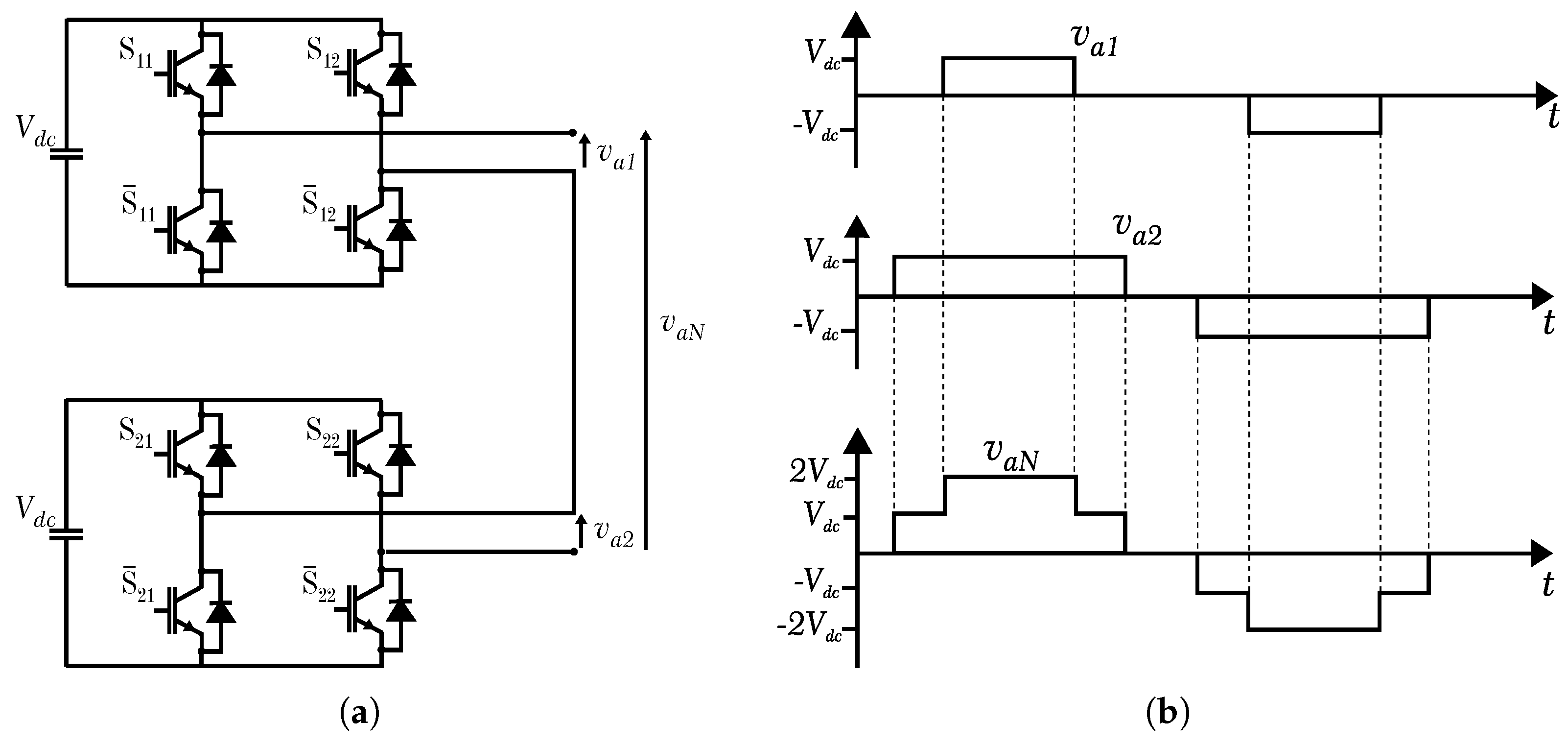
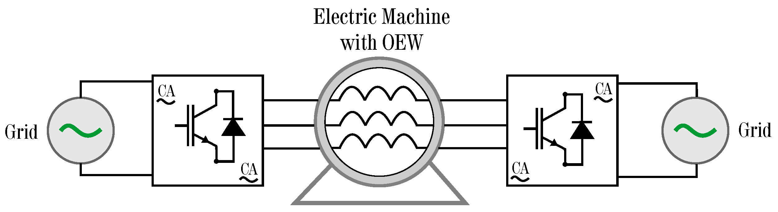
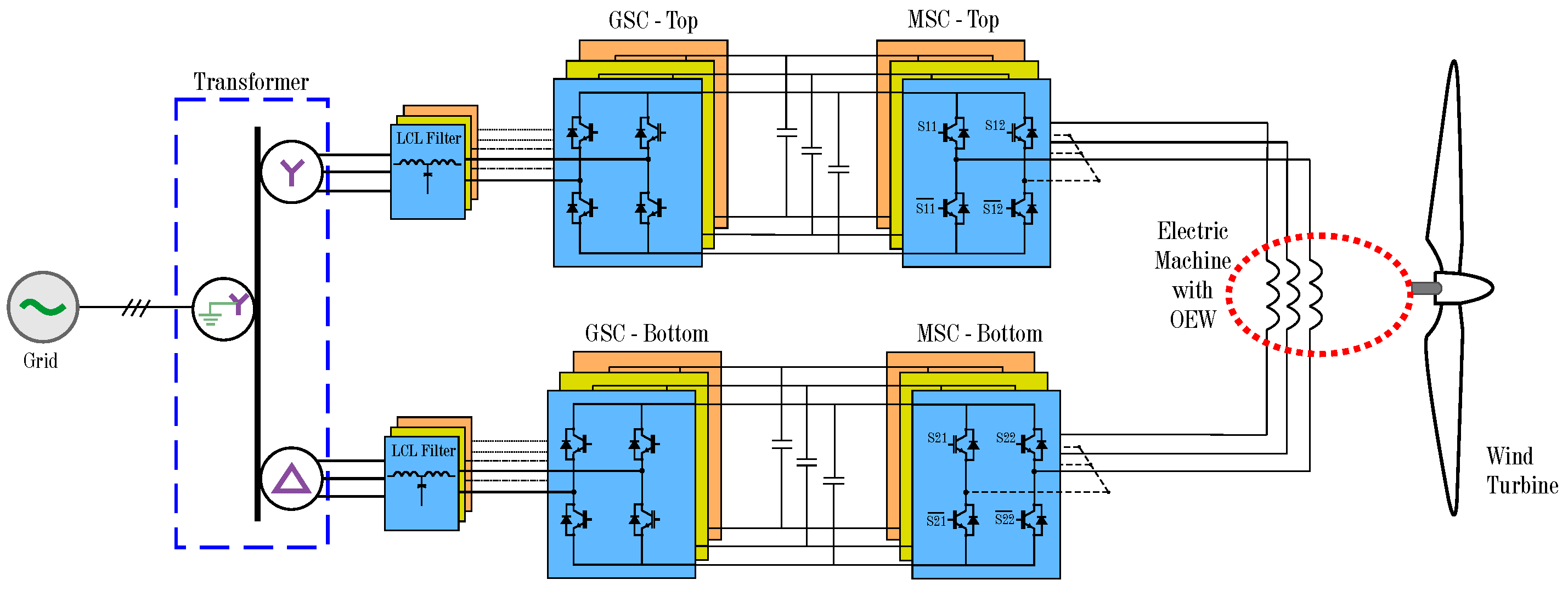
2.3. Multilevel Converter and Electric Machines with Open-End Windings
3. Proposed System
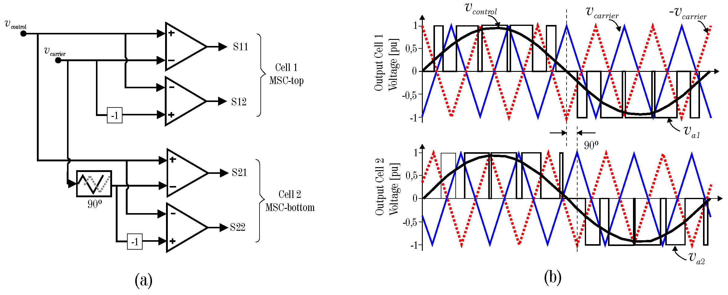
3.1. Modulation Strategy
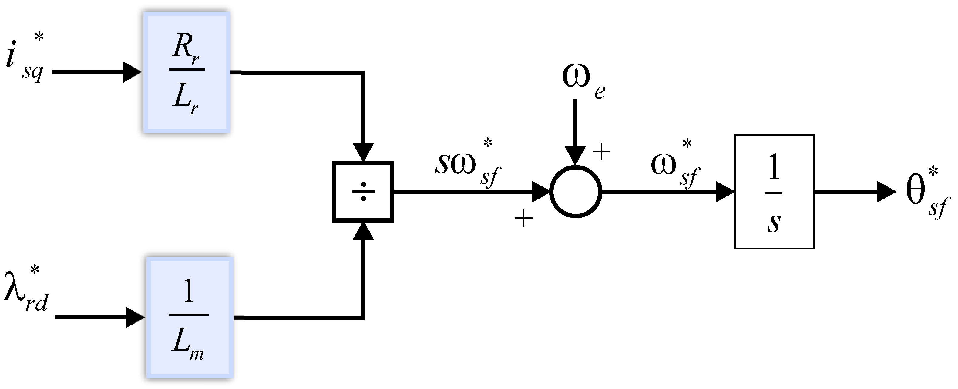
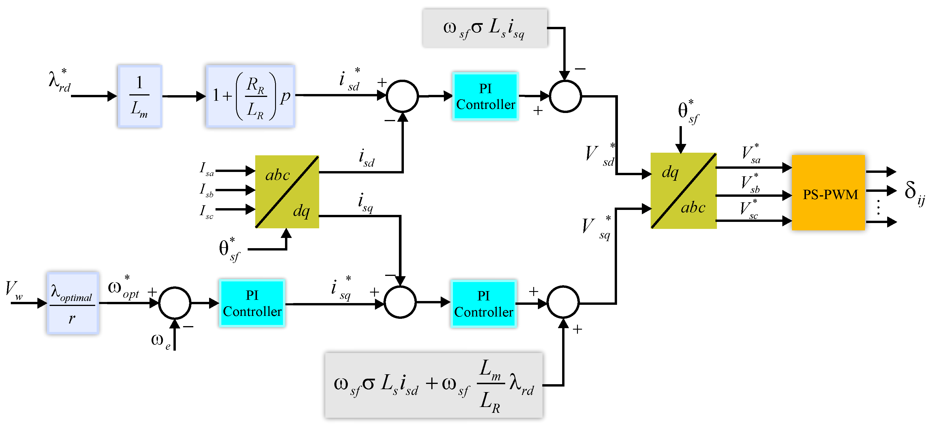
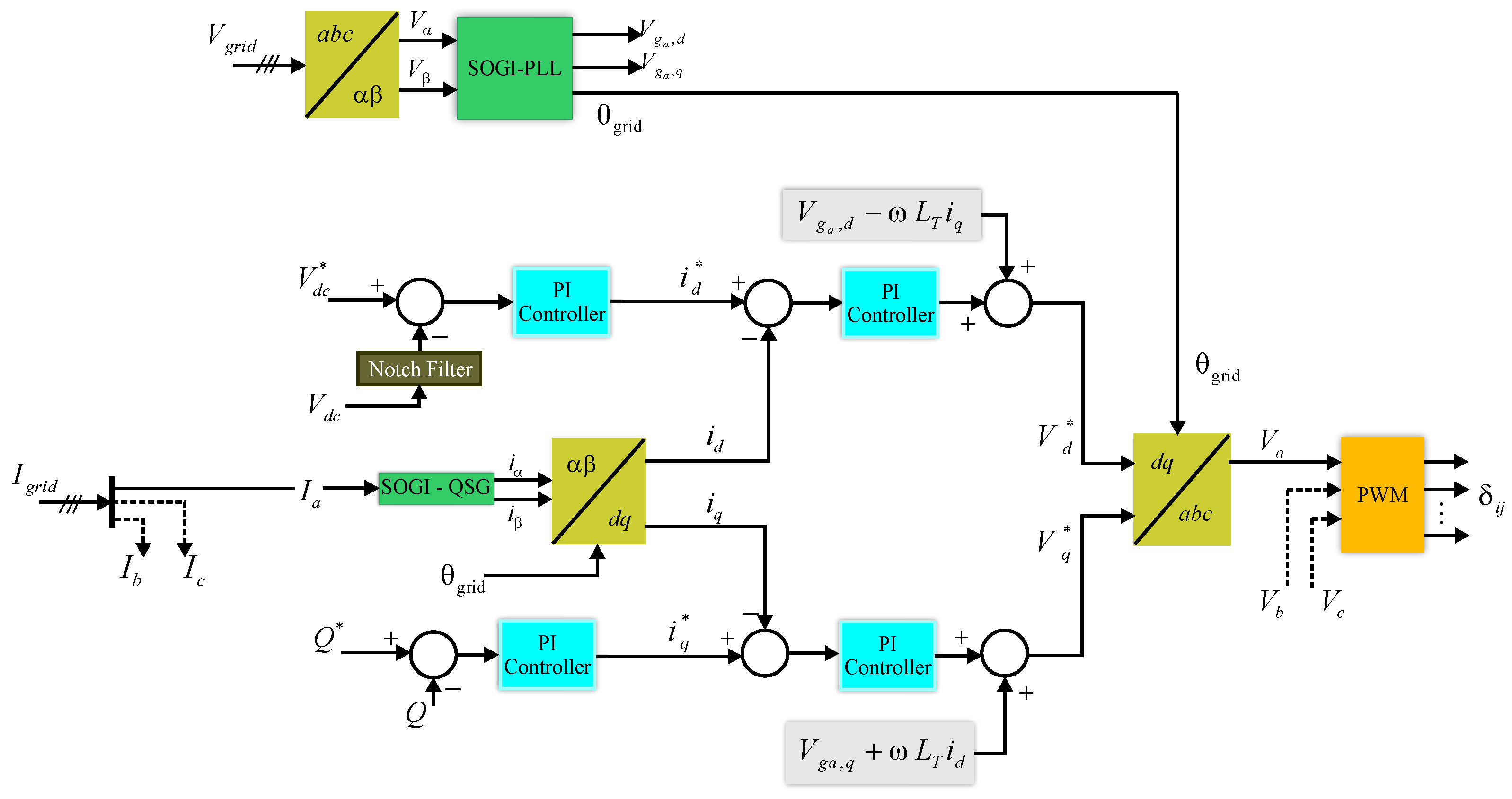
3.2. Control Strategies
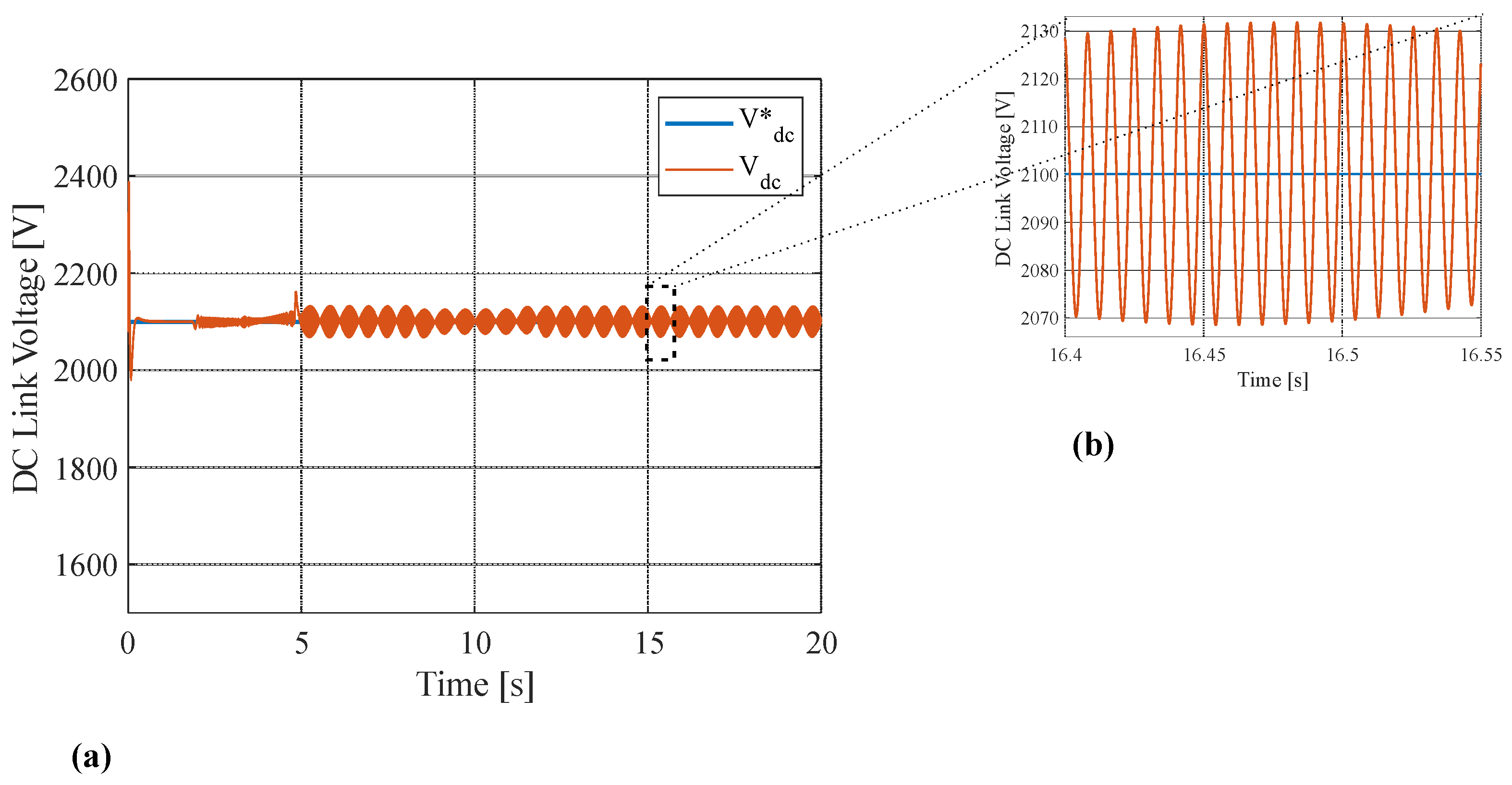
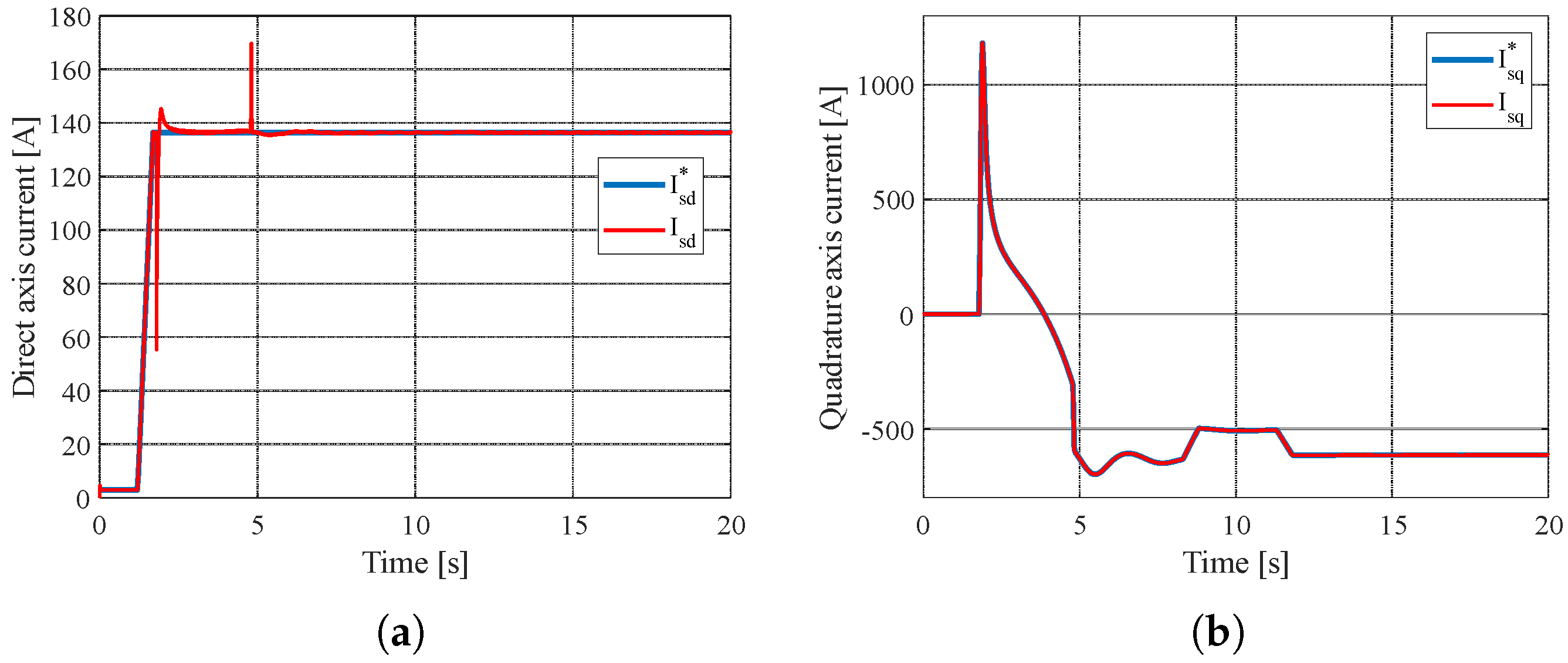
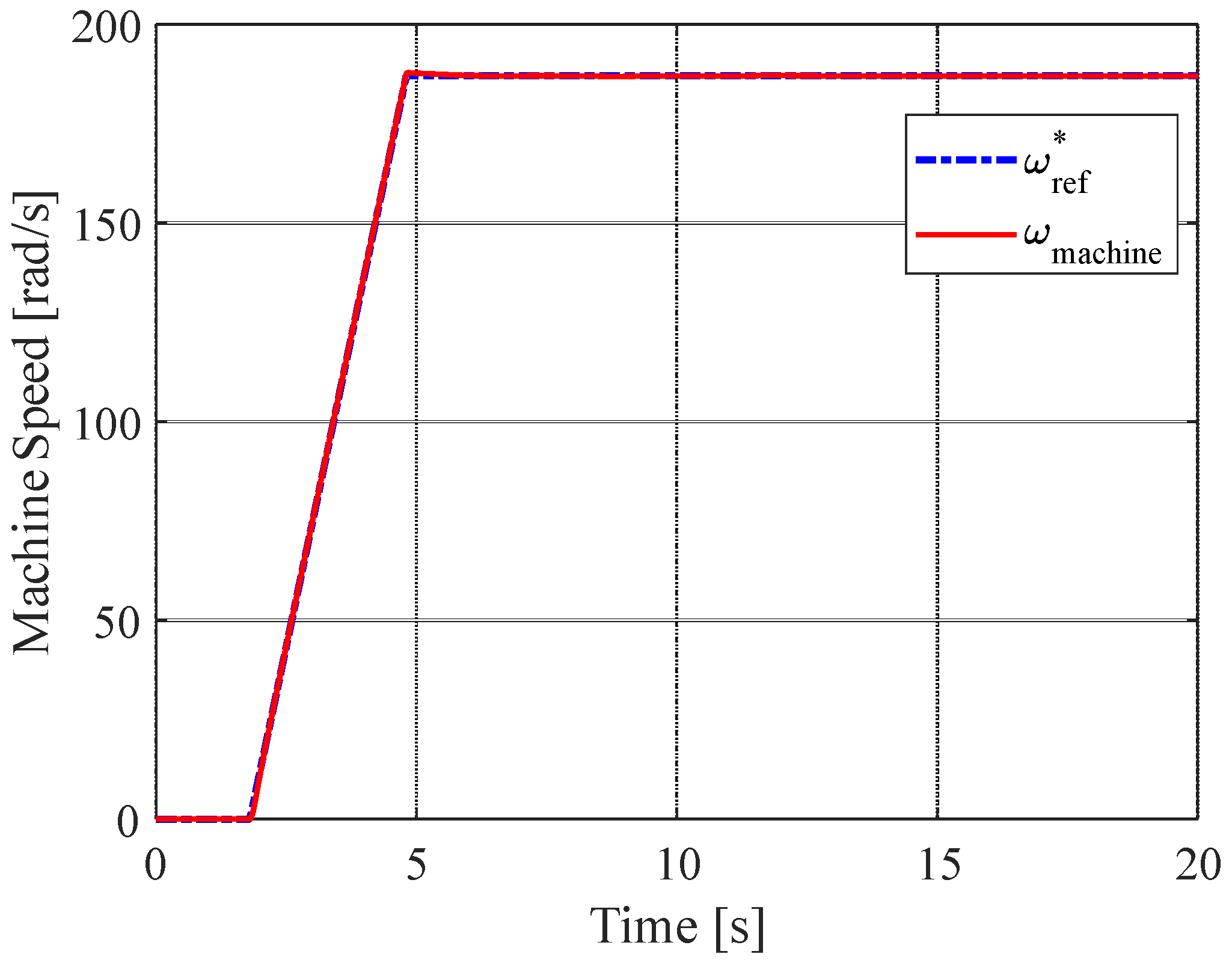
4. Results and Discussion
5. Conclusions
Author Contributions
Funding
Institutional Review Board Statement
Informed Consent Statement
Data Availability Statement
Conflicts of Interest
Abbreviations
| CHB | Cascaded H-Bridge |
| FC | Flying Capacitor |
| GSC | Grid-side Converter |
| MSC | Machine-side Converter |
| NPC | Neutral Point Clamped |
| OEW | Open-end Winding |
| SCIM | Squirrel-Cage Induction Machine |
| WECS | Wind Energy Conversion System |
References
- GWEC. Global Wind Report 2022. Available online: https://gwec.net/wp-content/uploads/2022/03/GWEC-GLOBAL-WIND-REPORT-2022.pdf (accessed on 16 January 2023).
- REN21. Renewables 2022 Global Status Report. Available online: https://www.ren21.net/wp-content/uploads/2019/05/GSR2022_Full_Report.pdf (accessed on 16 January 2023).
- Franquelo, L.G.; Rodriguez, J.; Leon, J.I.; Kouro, S.; Portillo, R.; Prats, M.A. The age of multilevel converters arrives. IEEE Ind. Electron. Mag. 2008, 2, 28–39. [Google Scholar] [CrossRef]
- Kouro, S.; Malinowski, M.; Gopakumar, K.; Pou, J.; Franquelo, L.G.; Wu, B.; Rodriguez, J.; Pérez, M.A.; Leon, J.I. Recent advances and industrial applications of multilevel converters. IEEE Trans. Ind. Electron. 2010, 57, 2553–2580. [Google Scholar] [CrossRef]
- Ma, K.; Blaabjerg, F. Multilevel converters for 10 MW wind turbines. In Proceedings of the 2011-14th European Conference on Power Electronics and Applications (EPE 2011), Birmingham, UK, 30 August–1 September 2011; pp. 1–10. [Google Scholar]
- Rodriguez, J.; Franquelo, L.G.; Kouro, S.; Leon, J.I.; Portillo, R.C.; Prats, M.A.M.; Perez, M.A. Multilevel converters: An enabling technology for high-power applications. Proc. IEEE 2009, 97, 1786–1817. [Google Scholar] [CrossRef]
- Nabae, A.; Takahashi, I.; Akagi, H. A New Neutral-Point-Clamped PWM Inverter. IEEE Trans. Ind. Appl. 1981, IA-17, 518–523. [Google Scholar] [CrossRef]
- Meynard, T.A.; Foch, H. Multi-Level Choppers for High Voltage Applications. Epe J. 1992, 2, 45–50. [Google Scholar] [CrossRef]
- Kedika, N.R.; Pradabane, S. Fault-tolerant multi-level inverter topologies for open-end winding induction motor drive. Int. Trans. Electr. Energy Syst. 2021, 31, 12718. [Google Scholar] [CrossRef]
- Marchesoni, M.; Mazzucchelli, M.; Tenconi, S. A non conventional power converter for plasma stabilization. In Proceedings of the PESC ’88 Record, 19th Annual IEEE Power Electronics Specialists Conference, Kyoto, Japan, 11–14 April 1988; Volume 1, pp. 122–129. [Google Scholar] [CrossRef]
- Osman, R. A medium-voltage drive utilizing series-cell multilevel topology for outstanding power quality. In Proceedings of the Conference Record of the 1999 IEEE Industry Applications Conference. Thirty-Forth IAS Annual Meeting (Cat. No.99CH36370), Phoenix, AZ, USA, 3–7 October 1999; Volume 4, pp. 2662–2669. [Google Scholar] [CrossRef]
- Blaabjerg, F.; Liserre, M.; Ma, K. Power Electronics Converters for Wind Turbine Systems. IEEE Trans. Ind. Appl. 2012, 48, 708–719. [Google Scholar] [CrossRef]
- Ma, K.; Blaabjerg, F.; Xu, D. Power devices loading in multilevel converters for 10 MW wind turbines. In Proceedings of the 2011 IEEE International Symposium on Industrial Electronics, Gdansk, Poland, 27–30 June 2011; pp. 340–346. [Google Scholar] [CrossRef]
- Pires, V.F.; Foito, D.; Silva, J.F. Fault-Tolerant Multilevel Topology Based on Three-Phase H-Bridge Inverters for Open-End Winding Induction Motor Drives. IEEE Trans. Energy Convers. 2017, 32, 895–902. [Google Scholar] [CrossRef]
- Stemmler, H.; Guggenbach, P. Configurations of high-power voltage source inverter drives. In Proceedings of the Fifth European Conference on Power Electronics and Applications, Brighton, UK, 13–16 September 1993; Volume 5, pp. 7–14. [Google Scholar]
- Hong, J.; Lee, H.; Nam, K. Charging Method for the Secondary Battery in Dual-Inverter Drive Systems for Electric Vehicles. Proc. IEEE Trans. Power Electron. 2015, 30, 909–921. [Google Scholar] [CrossRef]
- Jain, S.; Thopukara, A.K.; Karampuri, R.; Somasekhar, V.T. A Single-Stage Photovoltaic System for a Dual-Inverter-Fed Open-End Winding Induction Motor Drive for Pumping Applications. IEEE Trans. Power Electron. 2015, 30, 4809–4818. [Google Scholar] [CrossRef]
- Rajeevan, P.P.; Sivakumar, K.; Gopakumar, K.; Patel, C.; Abu-Rub, H. A Nine-Level Inverter Topology for Medium-Voltage Induction Motor Drive With Open-End Stator Winding. IEEE Trans. Ind. Electron. 2013, 60, 3627–3636. [Google Scholar] [CrossRef]
- Somasekhar, V.; Baiju, M.; Mohapatra, K.; Gopakumar, K. A multilevel inverter system for an induction motor with open-end windings. In Proceedings of the IEEE 2002 28th Annual Conference of the Industrial Electronics Society. IECON 02, Seville, Spain, 5–8 November 2002; Volume 2, pp. 973–978. [Google Scholar] [CrossRef]
- Matos, F.F.V.; Ramos, H.d.O.; Rocha, D.C.G.; da Silva, R.M.; Mendes, M.A.S.; Mendes, V.F. A multilevel wind power conversion system with an open winding squirrel cage induction generator. In Proceedings of the 2015 IEEE 13th Brazilian Power Electronics Conference and 1st Southern Power Electronics Conference (COBEP/SPEC), Fortaleza, Brazil, 29 November–2 December 2015; pp. 1–6. [Google Scholar] [CrossRef]
- Ricardi, V.; Ferreira Viana Matos, F.; Rodrigues de Jesus, V.M.; de Sousa, C.V.; de Almeida Zica, L.E.L.; Mendes, V.F. Control and operation of open-end winding permanent magnet synchronous wind generator. In Proceedings of the 2017 Brazilian Power Electronics Conference (COBEP), Luiz de Fora, Brazil, 19–22 November 2017; pp. 1–6. [Google Scholar] [CrossRef]
- Vattuone, L.; Kouro, S.; Estay, G.; Wu, B. Open-end-winding PMSG for wind energy conversion system with dual boost NPC converter. In Proceedings of the 2013 IEEE International Conference on Industrial Technology (ICIT), Cape Town, South Africa, 25–28 February 2013; pp. 1763–1768. [Google Scholar] [CrossRef]
- Xing, N.; Hu, S.; Lin, Z.; Tan, Z.; Cao, W.; Gadoue, S. New Adaptive Control Strategies for Open-End Winding Permanent Magnet Synchronous Generator (OEW-PMSG) for Wind Power Generation. In Proceedings of the The 10th International Conference on Power Electronics, Machines and Drives (PEMD 2020), Virtual, 15–17 December 2020; Volume 2020, pp. 838–843. [Google Scholar] [CrossRef]
- Matos, F.F.; Mendes, M.A.; Meynard, T.; Mendes, V.F. A generalized open-end winding conversion system using flying capacitor cells. Electr. Power Syst. Res. 2019, 169, 174–183. [Google Scholar] [CrossRef]
- Rodríguez, J.; Bernet, S.; Wu, B.; Pontt, J.O.; Kouro, S. Multilevel voltage-source-converter topologies for industrial medium-voltage drives. IEEE Trans. Ind. Electron. 2007, 54, 2930–2945. [Google Scholar] [CrossRef]
- Teodorescu, R.; Liserre, M.; Rodríguez, P. Grid Converters for Photovoltaic and Wind Power Systems; Wiley: London, UK, 2011. [Google Scholar]
- Orłowska-Kowalska, T.; Blaabjerg, F.; Rodríguez, J. Advanced and Intelligent Control in Power Electronics and Drives; Springer: Cham, Switzerland, 2014. [Google Scholar]
- Vas, P. Vector Control of AC Machines; Oxford University Press: Cary, NC, USA, 1990. [Google Scholar]
- Jacobina, C.B.; Rocha, N.; Marinus, N.S.M.L. Open-end winding permanent magnet synchronous generator system with reduced controlled switch count. In Proceedings of the 2013 Brazilian Power Electronics Conference, Gramado, Brazil, 27–31 October 2013; pp. 692–698. [Google Scholar] [CrossRef]
- Sivakumar, K.; Das, A.; Ramchand, R.; Patel, C.; Gopakumar, K. A three level voltage space vector generation for open end winding IM using single voltage source driven dual two-level inverter. In Proceedings of the TENCON 2009—2009 IEEE Region 10 Conference, Singapore, 23–26 November 2009; pp. 1–5. [Google Scholar] [CrossRef]
- Darvish Falehi, A. Half-cascaded multilevel inverter coupled to photovoltaic power source for AC-voltage synthesizer of dynamic voltage restorer to enhance voltage quality. Int. Numer. Model. Electron. Networks, Devices Fields 2021, 34, e2883. [Google Scholar] [CrossRef]
- Farakhor, A.; Reza Ahrabi, R.; Ardi, H.; Najafi Ravadanegh, S. Symmetric and asymmetric transformer based cascaded multilevel inverter with minimum number of components. IET Power Electron. 2015, 8, 1052–1060. [Google Scholar] [CrossRef]
- Fazel, S.S.; Bernet, S.; Krug, D.; Jalili, K. Design and comparison of 4-kV neutral-point-clamped, flying-capacitor, and series-connected H-bridge multilevel converters. IEEE Trans. Ind. Appl. 2007, 43, 1032–1040. [Google Scholar] [CrossRef]
- Rabiul Islam, M.; Mahfuz-Ur-Rahman, A.M.; Muttaqi, K.M.; Sutanto, D. State-of-the-Art of the Medium-Voltage Power Converter Technologies for Grid Integration of Solar Photovoltaic Power Plants. IEEE Trans. Energy Convers. 2019, 34, 372–384. [Google Scholar] [CrossRef]
- Blaabjerg, F.; Chen, Z. Power electronics for modern wind turbines. Synth. Lect. Power Electron. 2005, 1, 1–68. [Google Scholar]
- Novotny, D.; Lipo, T. Vector Control and Dynamics of AC Drives. In Monographs in Electrical and Electronic Engineering; Clarendon Press: Oxford, UK, 1996; Volume 41. [Google Scholar]
- Xia, Y.; Ahmed, K.H.; Williams, B.W. Wind Turbine Power Coefficient Analysis of a New Maximum Power Point Tracking Technique. IEEE Trans. Ind. Electron. 2013, 60, 1122–1132. [Google Scholar] [CrossRef]
- Heier, S. Grid Integration of Wind Energy: Onshore and Offshore Conversion Systems; Wiley: Hoboken, NJ, USA, 2014. [Google Scholar]
- Suul, J.A.; Molinas, M.; Norum, L.; Undeland, T. Tuning of control loops for grid connected voltage source converters. In Proceedings of the 2008 IEEE 2nd International Power and Energy Conference, Johor Bahru, Malaysia, 1–3 December 2008; pp. 797–802. [Google Scholar] [CrossRef]
- Mendes, V.F.; de Sousa, C.V.; Silva, S.; Rabelo, B.C.; Hofmann, W. Modeling and Ride-Through Control of Doubly Fed Induction Generators During Symmetrical Voltage Sags. IEEE Trans. Energy Convers. 2011, 26, 1161–1171. [Google Scholar] [CrossRef]
- Rodríguez, P.; Teodorescu, R.; Candela, I.; Timbus, A.V.; Liserre, M.; Blaabjerg, F. New positive-sequence voltage detector for grid synchronization of power converters under faulty grid conditions. In Proceedings of the 2006 37th IEEE Power Electronics Specialists Conference, Jeju, Republic of Korea, 18–22 June 2006; pp. 1–7. [Google Scholar] [CrossRef]
- Peña-Alzola, R.; Liserre, M.; Blaabjerg, F.; Ordonez, M.; Yang, Y. LCL-Filter Design for Robust Active Damping in Grid-Connected Converters. IEEE Trans. Ind. Inform. 2014, 10, 2192–2203. [Google Scholar] [CrossRef]
- Infineon. Datasheet of Module FZ825R33HE4D. Available online: https://www.infineon.com/dgdl/Infineon-FZ825R33HE4D-DataSheet-v01_30-EN.pdf?fileId=5546d46278d64ffd0178f97d4dd50584 (accessed on 15 February 2023).
- Infineon. Datasheet of Module FF450R33T3E3. Available online: https://www.infineon.com/dgdl/Infineon-FF450R33T3E3-DataSheet-v01_20-EN.pdf?fileId=5546d46254bdc4f50154c8080a4e59f5 (accessed on 15 February 2023).
- Paul, C.; Krause, O.W.; Sudhoff, S.D. Analysis of Electric Machinery and Drive Systems; IEEE Press Series on Power Engineering; Wiley: Hoboken, NJ, USA, 2002. [Google Scholar]


| Switching States | Output Voltage (Phase A) | |||
|---|---|---|---|---|
| 1 | 0 | 1 | 0 | |
| 0 | 0 | 1 | 0 | |
| 1 | 0 | 0 | 0 | |
| 1 | 0 | 1 | 1 | |
| 1 | 1 | 1 | 0 | |
| 0 | 0 | 0 | 0 | 0 |
| 0 | 0 | 1 | 1 | |
| 0 | 1 | 1 | 0 | |
| 1 | 0 | 0 | 1 | |
| 1 | 1 | 0 | 0 | |
| 1 | 1 | 1 | 1 | |
| 0 | 0 | 0 | 1 | |
| 0 | 1 | 0 | 0 | |
| 0 | 1 | 1 | 1 | |
| 1 | 1 | 0 | 1 | |
| 0 | 1 | 0 | 1 | |
| Multilevel Converter | Advantages | Disadvantage |
|---|---|---|
| NPC | ||
| FC |
| |
| CHB |
| Parameter | Value |
|---|---|
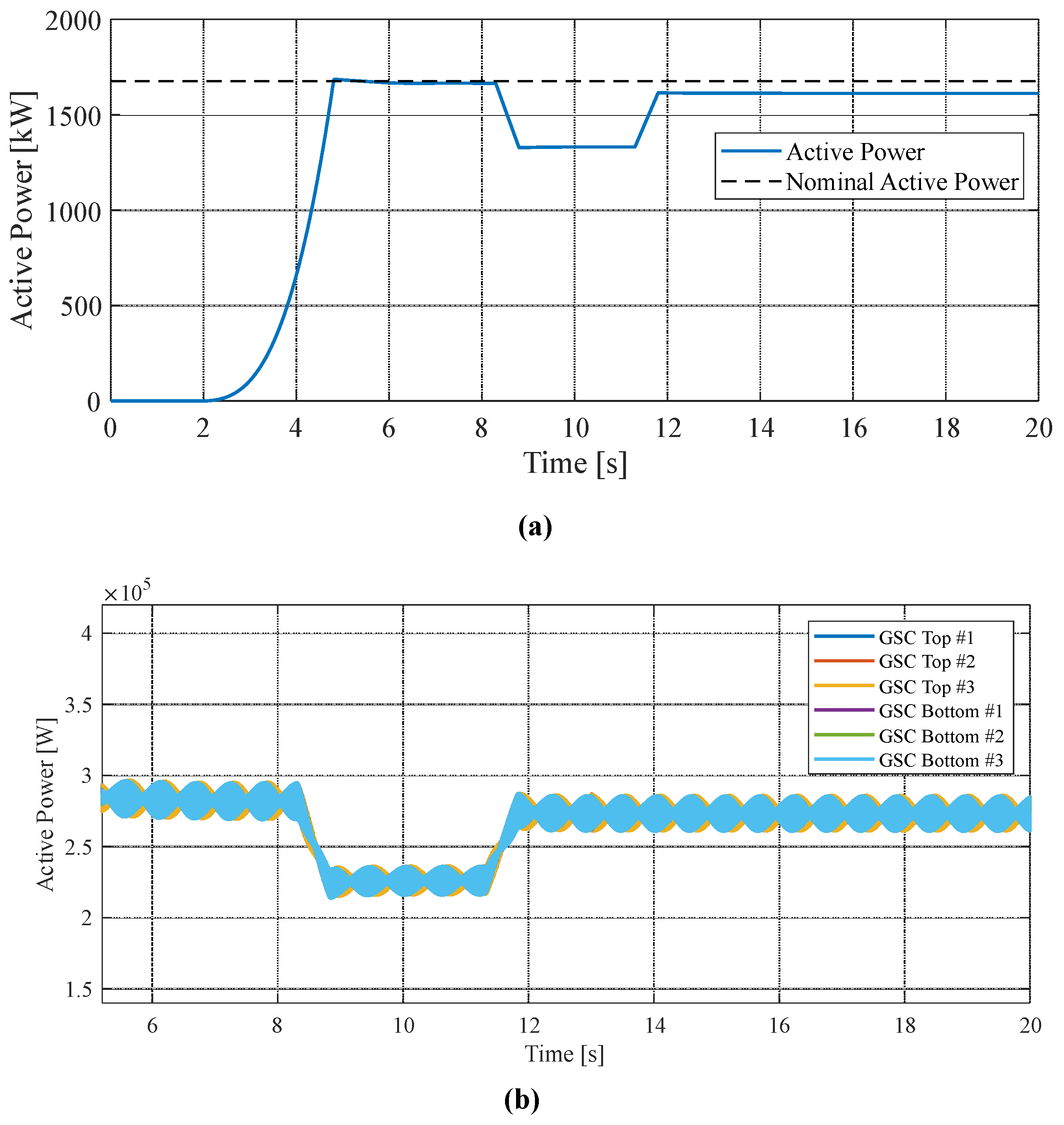
| Rated output power | 1677 kW |
| Nominal line stator voltage | 2300 V(rms) |
| Nominal stator current | 421.2 A(rms) |
| Nominal Frequency | 60 Hz |
| Nominal rotor speed | 1786 rpm |
| Number of poles pairs | 2 |
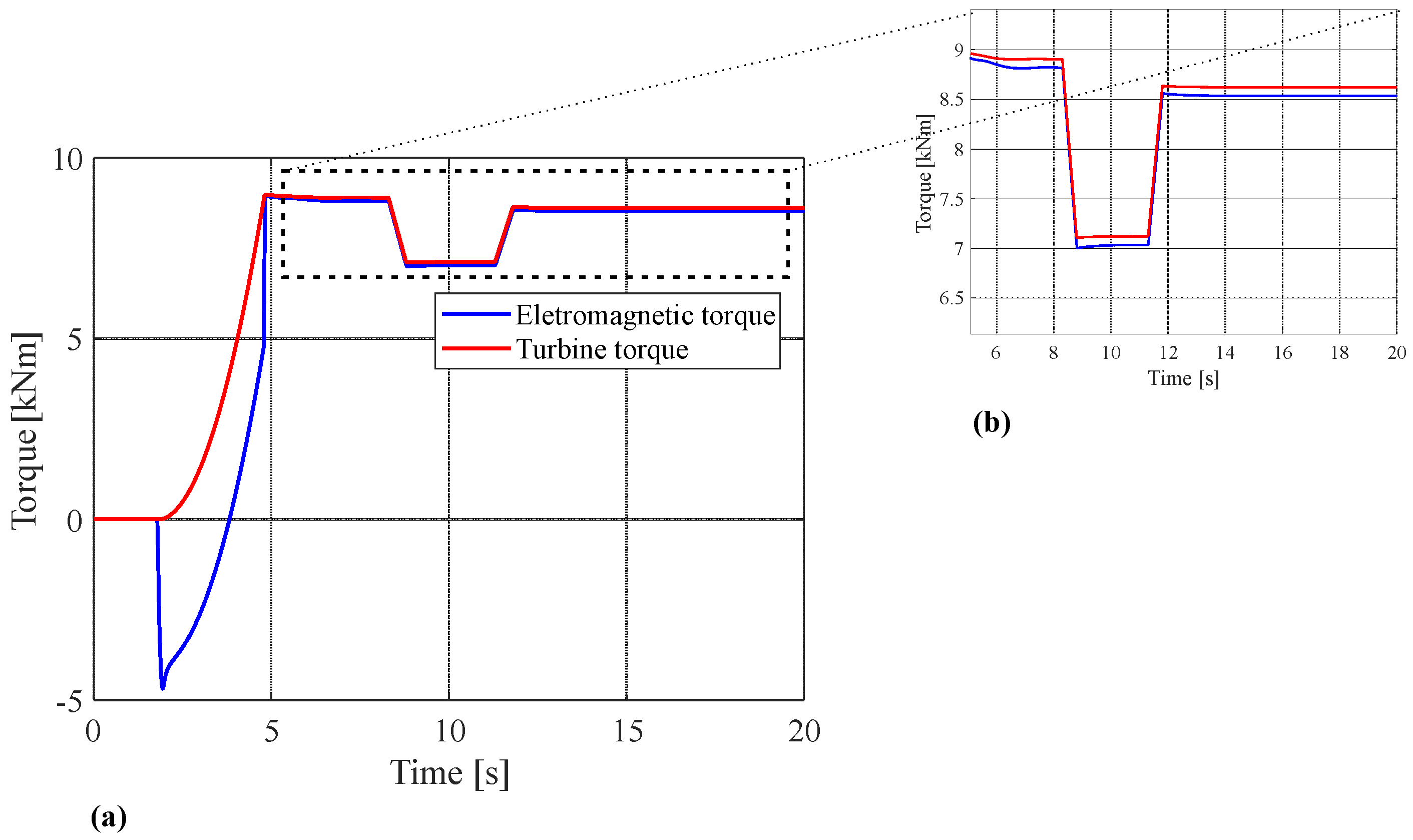
| Rated mechanical torque | 8.9 kNm |
| Stator winding resistance, | 29 m |
| Rotor winding resistance, | 22 m |
| Stator leakage reactance, | 0.226 m |
| Rotor leakage reactance, | 0.226 m |
| Magnetization reactance, | 13.04 m |
| Moment of inertia | 63.87 kgm |
| Nominal line grid voltage | 1150 V(rms) |
| Nominal grid frequency | 60 Hz |
| DC-link Voltage | 2100 V |
| DC-link Capacitance | 12 mF |
| Switching frequency (MSC and GSC) | 5 kHz |
| Converter side inductor, | 6.3 mH |
| Converter side resistor, | 23.8 m |
| Grid side inductor, | 0.63 mH |
| Grid side resistor, | 23.8 m |
| Parallel capacitor, C | 10.03 |
| Damping resistor, | 2.52 m |
| Description | Time |
|---|---|
| Start of simulation | 0.0 s |
| Machine magnetization start at | 1.2 s |
| Machine acceleration starts at | 1.8 s |
| Machine reaches the rated speed at | 5.0 s |
| Reduce equivalent to in machine torque at | 8.3 s |
| Increase of approximately in machine torque at | 11.3 s |
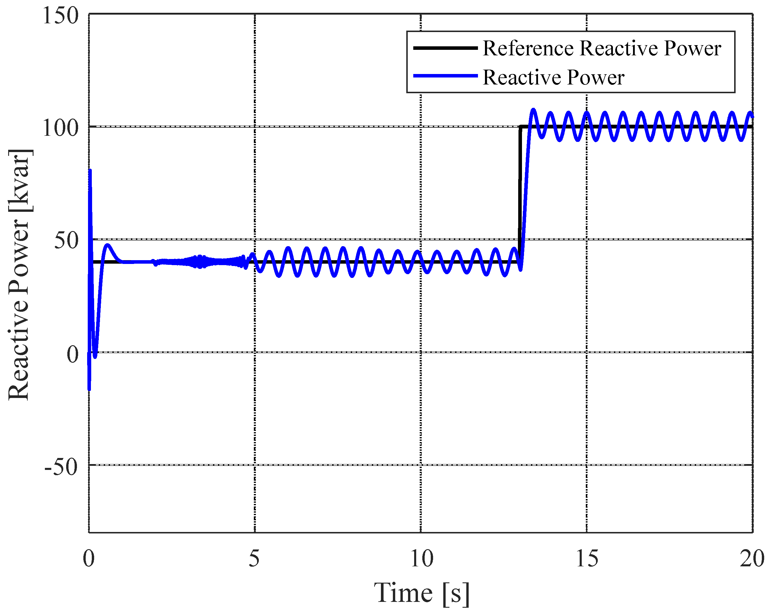
| Reactive power injection at | 13.0 s |
Disclaimer/Publisher’s Note: The statements, opinions and data contained in all publications are solely those of the individual author(s) and contributor(s) and not of MDPI and/or the editor(s). MDPI and/or the editor(s) disclaim responsibility for any injury to people or property resulting from any ideas, methods, instructions or products referred to in the content. |
© 2023 by the authors. Licensee MDPI, Basel, Switzerland. This article is an open access article distributed under the terms and conditions of the Creative Commons Attribution (CC BY) license (https://creativecommons.org/licenses/by/4.0/).
Share and Cite
Bettoni, S.d.S.; Ramos, H.d.O.; Matos, F.F.; Mendes, V.F. Cascaded H-Bridge Multilevel Converter Applied to a Wind Energy Conversion System with Open-End Winding. Wind 2023, 3, 232-252. https://doi.org/10.3390/wind3020014
Bettoni SdS, Ramos HdO, Matos FF, Mendes VF. Cascaded H-Bridge Multilevel Converter Applied to a Wind Energy Conversion System with Open-End Winding. Wind. 2023; 3(2):232-252. https://doi.org/10.3390/wind3020014
Chicago/Turabian StyleBettoni, Samuel dos Santos, Herbert de Oliveira Ramos, Frederico F. Matos, and Victor Flores Mendes. 2023. "Cascaded H-Bridge Multilevel Converter Applied to a Wind Energy Conversion System with Open-End Winding" Wind 3, no. 2: 232-252. https://doi.org/10.3390/wind3020014