Preconditioned Monte Carlo for Gradient-Free Bayesian Inference in the Physical Sciences ^†

Abstract

We present preconditioned Monte Carlo (PMC), a novel Monte Carlo method for Bayesian inference in complex probability distributions. PMC incorporates a normalizing flow (NF) and an adaptive Sequential Monte Carlo (SMC) scheme, along with a novel past resampling scheme to boost the number of propagated particles without extra computational costs. Additionally, we utilize preconditioned Crank–Nicolson updates, enabling PMC to scale to higher dimensions without the gradient of target distribution. The efficacy of PMC in producing samples, estimating model evidence, and executing robust inference is showcased through two challenging case studies, highlighting its superior performance compared to conventional methods.

1. Introduction

Bayesian inference (BI) is a crucial tool in the physical sciences, offering a mathematical framework for quantifying uncertainty [1,2,3,4,5]. BI rests on three core elements: prior and posterior distributions, and the likelihood function. The prior distribution encapsulates our initial understanding of a problem, representing our beliefs before any data are observed. The likelihood function signifies how likely it is our observed data are under varying model parameters. Posterior distributions emerge from Bayes’ theorem, combining the prior and likelihood to update our beliefs after data observation.

However, most BI analyses are analytically intractable, demanding numerical methods such as Markov chain Monte Carlo (MCMC). These techniques approximate the posterior, generating samples from it. State-of-the-art MCMC methods hinge on the knowledge of the gradient of the target probability density, which is often intractable in the physical sciences. Moreover, MCMC faces other challenges: its inherently serial nature makes parallelization difficult, it struggles with multimodal or highly correlated distributions, and it is generally unable to compute the marginal likelihood, a critical component for model comparison. These limitations underscore the need for more flexible and efficient computational tools.

Sequential Monte Carlo (SMC) is a Monte Carlo method designed to address these challenges [6,7,8]. SMC distinguishes itself with straightforward parallelization, an ability to handle multimodal posteriors, and the provision of a marginal likelihood estimate. In SMC, MCMC acts as a tool for moving the particles, typically utilizing gradient-free MCMC variants, such as random-walk metropolis (RWM) [9] and slice sampling (SS) [10]. Despite its advantages, the SMC based on these MCMC methods still struggles to scale to high-dimensional problems and handle highly correlated and multimodal posteriors.

To overcome these challenges, we introduce preconditioned Monte Carlo (PMC), a refined variant of SMC. PMC employs a normalizing flow (NF) [11] to Gaussianize the target distribution, simplifying MCMC sampling [12,13,14]. In contrast to canonical SMC, PMC includes a novel resampling scheme termed past resampling (PR), enhancing the number of propagated particles without incurring additional computational costs. Furthermore, PMC departs from the reliance on RWM or SS for sampling, instead choosing preconditioned Crank–Nicolson (pCN) updates [15,16]. As such, PMC can scale to higher dimensions without requiring the gradient of the target distribution, enhancing the overall sampling performance.

2. Methods

2.1. Sequential Monte Carlo

2.1.1. Background

Sequential Monte Carlo (SMC) propagates a set of particles, drawn from a known distribution $\rho (\theta )$, through multiple intermediary distributions towards a target distribution $p(\theta )$. The transition speed depends on the number of intermediary distributions. Like annealed importance sampling (AIS), SMC uses multiple MCMC steps per iteration to balance particles towards each stage’s equilibrium distribution. SMC differentiates from AIS by employing resampling to avoid weight degeneracy, where a few particles hold high-importance weights. The resampling equalizes the weights to manage their high variance.

2.1.2. Bridging the Prior and Posterior

To develop a series of intermediate distributions that help the transition from a known initial distribution $\rho (\theta )$ to the desired posterior distribution $p(\theta )$, a method of interpolation is typically employed as follows:

$$p_t(\theta )\propto {\rho }^{1-{\beta }_t}(\theta )p^{{\beta }_t}(\theta ),t=1,\dots ,m$$

(1)

where ${\beta }_t$ refers to a sequence of annealing temperatures, arranged such that

$$0={\beta }_1<{\beta }_2<\cdots <{\beta }_m=1$$

(2)

In a Bayesian setting, the prior is naturally chosen as the auxiliary density $\rho (\theta )=p(\theta |\mathcal{M})$, and the posterior as the target density $p(\theta )=p(\theta |d,\mathcal{M})$. In this case, Equation (1) simplifies to:

$$p_t(\theta )\propto p^{{\beta }_t}(d|\theta ,\mathcal{M})p(\theta |\mathcal{M})$$

(3)

2.1.3. Key Steps

The process of transitioning from one distribution to the next, $p_{t-1}(\theta )$ to $p_t(\theta )$, is performed in three primary steps: correction, selection, and mutation. These steps are encapsulated in a single SMC iteration, which is repeated until the target distribution is adequately approximated.

• Correction—The importance weights $w_t^i$ of the particles ${\theta }_{t-1}^i$ are calculated as:

  $$w_t^i=\frac{p_t({\theta }_{t-1}^i)}{p_{t-1}({\theta }_{t-1}^i)}$$

  (4)

  and then they are used to estimate the normalizing constant (i.e., marginal likelihood) of $p_t(\theta )$:

  $${\mathcal{Z}}_t={\mathcal{Z}}_{t-1}\times \frac{1}{N}{\displaystyle \sum _{i=1}^N}{w}_t^i$$

  (5)
  Initially, all weights are equal such that $w_1^i=1/N\forall i\in \{1,2,\dots ,N\}$ with ${\mathcal{Z}}_1=0$.
• Selection—the particles ${\theta }_{t-1}^i$ are resampled according to their importance weights. The goal is to retain those particles that are highly represented in the new distribution $p_t(\theta )$, while eliminating those that are less represented. Particles with high weights are more likely to be selected, thus forming the resampled set ${\theta }_t^i$.
• Mutation—The resampled particles ${\theta }_t^i$ are perturbed to generate diversity and explore more of the parameter space. This step uses a transition kernel $K_t({\theta }_t^i,{\theta }^{\prime })$. In practice, $K_t$ takes the form of an MCMC kernel (e.g., several steps of an Metropolis–Hastings (MH) transition). The careful design of the transition kernel is required to ensure that the SMC sampler maintains good mixing properties and computational efficiency.

2.1.4. Adaptive Temperature Schedule

The effective sample size (ESS) measures the number of statistically independent samples in the weighted ensemble. It provides an estimate of the “quality” of the samples and is given by:

$$ESS=\frac{1}{{\sum }_{i=1}^N{(w_t^i)}^2},$$

(6)

where the weights $w_t^i$ are normalized to sum to one. In practice, a constant ESS is maintained throughout the run by determining each ${\beta }_t$ adaptively by setting the next temperature level as:

$${\beta }_{t+1}=arg\underset{\beta }{min}\left\{\beta :ES{S}_{\beta }\ge ES{S}_{target}\right\},$$

(7)

where $ES{S}_{\beta }$ represents the effective sample size at a temperature of $\beta$, N is the total number of samples, and $ES{S}_{target}$ is the target ESS. The algorithm proceeds with the new temperature until the final target distribution (i.e., the posterior) is achieved. This adaptive temperature selection scheme, guided by ESS, is a common feature of SMC. This enables the efficient bridging of the gap between the prior and posterior while ensuring a diverse set of samples.

2.2. Past Resampling

In the canonical formulation of SMC, the new particles are resampled from the previous generation of particles with probabilities proportional to their importance weights given by Equation (4). However, this scheme exhibits several limitations. First, the number of particles, N, of a generation needs to be large enough to effectively capture the characteristics of the tempered distribution of the Equation (1). This effect is further exaggerated in higher dimensions. Secondly, the ESS${}_{target}$ needs to amount to a significant fraction of N (i.e., 80–99%) to suppress the high variance of the importance weights. Third, even when the N and ESS${}_{target}$ are large, the resampled particles will include many copies of the same particles. This requires running MCMC longer during the mutation stage to diversify these particles.

To address these challenges without increasing the computational cost of the method, we propose to resample particles from all past generations, instead of just the last one. We refer to this modification of SMC as past resampling (PR). As the number of resampled particles is substantially lower than that of the particles of past generations, $N^{\prime }$, the former are effectively independent and do not include copies of the same particle. This addresses the third challenges of the canonical approach. Furthermore, the target ESS, which determines the convergence rate of the algorithm, can be significantly higher than in the canonical formulation, addressing the first and second issues.

PR requires the computation of importance weights for the particles of all (or a subset of) past iterations. In the $t_{th}$ iteration, the weights of the particles of the $t_{th}^{\prime }$ iteration can be written as:

$$w_{t{t}^{\prime }}^i={\Lambda }_{t{t}^{\prime }}{\tilde{W}}_{t{t}^{\prime }}^i,$$

(8)

where ${\tilde{W}}_{t{t}^{\prime }}^i$ are the normalized importance weights:

$${\tilde{W}}_{t{t}^{\prime }}^i=\frac{{\tilde{w}}_{t{t}^{\prime }}^i}{{\sum }_{i=1}^N{\tilde{w}}_{t{t}^{\prime }}^i},$$

(9)

where:

$${\tilde{w}}_{t{t}^{\prime }}^i=\frac{p_t({\theta }_{t^{\prime }})}{p_{t^{\prime }}({\theta }_{t^{\prime }})}.$$

(10)

The coefficients ${\Lambda }_{t{t}^{\prime }}$ determine the influence of past iterations on the current one. Generally, the further in the past $t^{\prime }$ is, the less significant its influence. The estimation of ${\Lambda }_{t{t}^{\prime }}$ can be formulated as the variational calculus problem of maximizing the total ESS. The solution of this problem leads to:

$${\Lambda }_{t{t}^{\prime }}=\frac{{\lambda }_{t{t}^{\prime }}}{{\sum }_{t^{\prime }=1}^t{\lambda }_{t{t}^{\prime }}},$$

(11)

where:

$${\lambda }_{t{t}^{\prime }}=\frac{1}{{\sum }_{i=1}^N{\left({\tilde{W}}_{t{t}^{\prime }}^i\right)}^2}.$$

(12)

In other words, the importance weights of the particles of the $t_{th}^{\prime }$ iteration with respect to the current $t_{th}$ iteration are adjusted by the normalized ESS given by Equation (11). Equations (8)–(12) are related to the recycling scheme proposed by [17,18] and applied at the end of the run. The main difference is that PR is applied to every iteration of SMC, instead of just the last one. In practice, only the iterations with ${\lambda }_{t{t}^{\prime }}>10$ are used to avoid noisy contributions.

The weights of Equation (8) can be employed to design a lower-variance estimate of the normalizing constant of $p_t(\theta )$, which generalizes Equation (5):

$${\mathcal{Z}}_t={\displaystyle \sum _{t^{\prime }=1}^{t-1}}\left({\Lambda }_{t{t}^{\prime }}{\mathcal{Z}}_{t^{\prime }}\frac{1}{N}{\displaystyle \sum _{i=1}^N}{\tilde{w}}_{t{t}^{\prime }}^i\right)$$

(13)

2.3. Preconditioning

2.3.1. Background

The mutation step of SMC typically involves the use of the MH algorithm. MH comprises a general class of MCMC methods that generate samples, in the form of a Markov chain, from the target distribution $p_{\theta }(\theta )$ by iterating a proposal and acceptance step. In the proposal step, a new state ${\theta }^{\prime }$ is sampled from the proposal distribution $q_{\theta }({\theta }^{\prime }|\theta )$, that is, conditioned on the current state $\theta$ in the Markov chain. In the acceptance step, the new state is added to the Markov chain with a probability given by:

$$\alpha =min\left\{1,\frac{p_{\theta }({\theta }^{\prime })q_{\theta }(\theta |{\theta }^{\prime })}{p_{\theta }(\theta )q_{\theta }({\theta }^{\prime }|\theta )}\right\}$$

(14)

If the new state is rejected, then the current state $\theta$ is added to the Markov chain instead and the process is repeated until a sufficient number of samples have been collected. The form of the acceptance probability of Equation (14) is designed to ensure detailed balance, a sufficient condition for the Markov chain to have $p_{\theta }(\theta )$ as its invariant distribution. In the case of SMC, the MH algorithm is employed during the mutation step targeting the current tempered distribution $p_t$.

The choice of a proposal distribution $q_{\theta }({\theta }^{\prime }|\theta )$ is crucial as it determines the overall sampling efficiency of the method. Generally, a good proposal distribution needs to balance exploration and exploitation, by generating states that are sufficiently different from the current one while maintaining a high acceptance rate. A common choice for $q_{\theta }({\theta }^{\prime }|\theta )$ is the normal distribution $N({\theta }^{\prime }|\theta ,C)$ leading to the RWM algorithm. The efficiency of RWM can be substantially improved by setting $C=2.{38}^2/D\times \Sigma$, where D is the number of dimensions and $\Sigma$ is the covariance matrix describing the target distribution $p_{\theta }(\theta )$.

However, if the target distribution $p_{\theta }(\theta )$ is significantly non-Gaussian, then the simple choice of $q_{\theta }({\theta }^{\prime }|\theta )=N({\theta }^{\prime }|\theta ,C)$ is insufficient and a more sophisticated proposal distribution is required. Designing advanced proposal distributions is an active field of research within the statistics community. The problem is further exaggerated in higher dimensions where the $2.{38}^2/D$ factor leads to vanishingly small steps in parameter space. We argue that the method of preconditioning coupled with the appropriate proposal distribution has the potential to address both of these issues.

The basic idea behind preconditioning is to transform the target distribution $p_{\theta }(\theta )$ into the simpler distribution $p_z(z)$ using a bijective transformation $z=f(\theta )$. The two probability densities are linked through the following transformation:

$$p_z(z)=p_{\theta }(\theta )\left|det\frac{\partial f^{-1}(z)}{\partial z}\right|$$

(15)

Sampling from $p_z(z)$ is generally easier than $p_{\theta }(\theta )$ due to its higher symmetry and simpler geometry. For instance, one may choose $z=f(\theta )$ such that $p_z(z)$ is approximately a standard normal distribution $\mathcal{N}(z|0,1)$. The MH algorithm is trivially generalized to the latent space of the preconditioning transformation with a proposal distribution $q_z(z^{\prime }|z)$ and an acceptance probability of:

$$\alpha =min\left\{1,\frac{p_z(z^{\prime })q_z(z|z^{\prime })}{p_z(z)q_z(z^{\prime }|z)}\right\}$$

(16)

2.3.2. Normalizing Flows

Normalizing flows (NFs) are a natural choice for the preconditioning transformation $z=f(\theta )$. NFs are bijective transformations typically parameterized using a neural network (NN) architecture. Generally, the forms of NN and NF have to be chosen carefully to maintain the reversibility of the transformation and the tractability of the Jacobian determinant in Equation (15). Recent developments have led to flexible NFs that are easily trained using samples from $p_{\theta }(\theta )$. Although not limited to this, NFs typically aim to map $p_{\theta }(\theta )$ to a standard normal distribution $\mathcal{N}(\theta |0,{\mathbb{1}}_D)$. The NF can be trained to approximate a certain probability density by minimizing the forward Kullback–Leibler (KL) divergence as the loss function:

$$L=-\frac{1}{N}\sum w_{i}logp({\theta }_i)$$

(17)

2.3.3. Preconditioned Crank–Nicolson

In principle, any MH method can be applied in the latent space of z targeting $p_z(z)$. Refs. [12,13,14] utilized RWM, whereas [19] employed the No U-Turn Sampler (NUTS). Despite their performance, those methods do not take full advantage of the symmetries of $p_z(z)$.

Preconditioned Crank–Nicolson (pCN) provides a more suitable alternative [15,16]. Assuming that the target density can be decomposed as:

$$p(\theta )\propto \mathcal{L}(\theta )\mathcal{N}(\theta |0,\Sigma )$$

(18)

where $\mathcal{L}(\theta )$ is the likelihood function and $\mathcal{N}(\theta |0,\Sigma )$ is the normal prior density, a new state is proposed as follows:

$${\theta }^{\prime }=\sqrt{1-{ϵ}^2}\theta +ϵv$$

(19)

where $v\sim \mathcal{N}(\theta |0,\Sigma )$ and $0<ϵ<1$. In the limit that $ϵ\to 1$, ${\theta }^{\prime }$ is a sample from the prior, whereas when $ϵ\to 0$, ${\theta }^{\prime }=\theta$. For values between 0 and 1, the proposed states shift towards zero. For a weak likelihood function, ${\theta }^{\prime }$ is shifted along the direction of the gradient, leading to higher acceptance rates. The acceptance criterion takes the form:

$$\alpha =min\left\{1,\frac{\mathcal{L}({\theta }^{\prime })}{\mathcal{L}(\theta )}\right\},$$

(20)

where the term corresponding to the prior density is missing, as the latter is already included in the proposal.

The main limitations of pCN are the assumptions of a normal prior and of a weak likelihood function. For pCN to be efficient, the prior density needs to dominate any contributions from the likelihood, thus maintaining the symmetry of the normal distribution. Preconditioned pCN (p${}^2$CN) allows us to bypass these difficulties. Given the approximately standard normal target density $p_z(z)$, the p${}^2$CN proposal is:

$$z^{\prime }=\sqrt{1-{ϵ}^2}z+ϵv,$$

(21)

where $v\sim \mathcal{N}(v|0,1)$. The acceptance probability of the new state is:

$$\alpha =min\left\{1,\frac{\tilde{\mathcal{L}}(z^{\prime })}{\tilde{\mathcal{L}}(z)}\right\},$$

(22)

where $\tilde{\mathcal{L}}(z)=p_z(z)/\mathcal{N}(z|0,1)$ is the pseudo-likelihood function, which reduces to the proper target density $p_z(z)$ in latent space when multiplied with the pseudo-prior $\mathcal{N}(v|0,1)$.

Unlike RWM, p${}^2$CN can scale to high dimensions. In fact, for a sufficiently preconditioned target distribution, p${}^2$CN exhibits a non-zero acceptance rate for $ϵ>0$, even in a very high D. The efficiency of the method solely relies on the capacity of the preconditioning transformation to map the target distribution to a standard normal density and the value of $ϵ$.

2.4. Preconditioned Monte Carlo

PMC seamlessly integrates the SMC framework, PR, and p${}^2$CN into a comprehensive algorithm, as illustrated in Algorithm 1. A noteworthy feature is the use of an NF as a preconditioner. PMC is primarily characterized by three key hyperparameters. The first is the ESS, which regulates the algorithm’s convergence rate, and is implicitly tied to the number of beta levels. The second is the number of resampled particles, a value that should ideally be lower than the ESS. The algorithm’s performance shows a relatively low sensitivity to variations in this parameter, provided that the number of resampled particles remains below half the ESS value. Lastly, the number of p${}^2$CN steps per iteration is set to:

$$M=\frac{D}{2}\times min{\left(1,\frac{2.38/\sqrt{D}}{ϵ}\right)}^{3/2}$$

(23)

where $ϵ$ was adjusted at the beginning of each iteration to yield an acceptance rate of $40\%$.

Algorithm 1 Preconditioned Monte Carlo

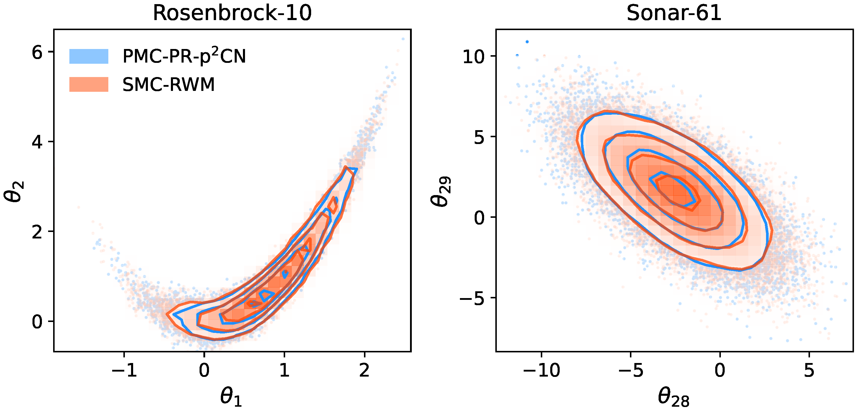
1: input Number of particles N and desired ESS 2: $t\leftarrow 1$, ${\beta }_1\leftarrow 0$, ${\mathcal{Z}}_1\leftarrow 1$, ${\{{\theta }_1^k\}}_{k=1}^N\sim \pi (\theta )$ 3: while   ${\beta }_t\ne 1$ do 4:    $t\leftarrow t+1$ 5:    ${\beta }_t\leftarrow$ solution to Equation (7) 6:    compute weights ${\{{\{w_{t{t}^{\prime }}^i\}}_{t^{\prime }=1}^t\}}_{i=1}^N$ using Equation (8) 7:    compute evidence ${\mathcal{Z}}_t$ using Equation (13) 8:    train $\theta =f(u)$ on ${\left\{{\{{\theta }_{t^{\prime }}^i,w_{t{t}^{\prime }}^i\}}_{t^{\prime }=1}^t\right\}}_{i=1}^N$ using Equation (17) 9:    ${\{{\tilde{\theta }}^i\}}_{i=1}^N\leftarrow$ resample N particles from ${\left\{{\{{\theta }_{t^{\prime }}^i,w_{t{t}^{\prime }}^i\}}_{t^{\prime }=1}^t\right\}}_{i=1}^N$ 10:    ${\{{\theta }_t^k\}}_{k=1}^N\leftarrow$ propagate ${\{{\tilde{\theta }}^i\}}_{i=1}^N$ according to ${\mathcal{K}}_t({\{{\theta }_t^i\}}_{i=1}^N\leftarrow {\{{\tilde{\theta }}_{t-1}^i\}}_{i=1}^N;f)$ 11: end while 12: return weighted samples ${\left\{{\{{\theta }_{t^{\prime }}^i,w_{t{t}^{\prime }}^i\}}_{t^{\prime }=1}^t\right\}}_{i=1}^N$ and estimate of the marginal likelihood ${\mathcal{Z}}_t$

3. Results

To verify the sampling performance of our approach, we perform an ablation study comparing PMC with PR and p${}^2$CN (PMC-PR-p${}^2$CN) to the following SMC variants: SMC with PR and RWM updates (SMC-PR-RWM), SMC with no PR and RWM updates (SMC-RWM), PMC with PR and RWM (PMC-PR-RWM), PMC with no PR and RWM (PMC-RWM), and PMC with no PR and p${}^2$CN (PMC-p${}^2$CN). The combinations of SMC with pCN were not included due to the low performance of pCN in the non-preconditioned setting. The total cost of each method in terms of likelihood evaluations along with the estimate of the logarithm of the marginal likelihood, $log\mathcal{Z}$, subtracted from the exact value, are shown in

Table 1. Computational cost in terms of the number of likelihood evaluations and marginal likelihood estimates.

Algorithm	Rosenbrock-10	Sonar-61	Rosenbrock-10	Sonar-61
	(Calls $\times {\mathbf{10}}^{\mathbf{6}}$)	(Calls $\times {\mathbf{10}}^{\mathbf{6}}$)	($\Delta \mathbf{log}\mathcal{Z}$)	($\Delta \mathbf{log}\mathcal{Z}$)
PMC-PR-p${}^2$CN	$\mathbf{0.11}$	$\mathbf{0.32}$	$\mathbf{0.09}\pm \mathbf{0.21}$	$-\mathbf{0.08}\pm \mathbf{0.12}$
PMC-PR-RWM	$0.23$	$2.31$	$0.18\pm 0.27$	$0.36\pm 0.69$
PMC-p${}^2$CN	0.21	$1.21$	$-0.33\pm 0.66$	$0.27\pm 0.38$
PMC-RWM	0.48	$6.41$	$-0.39\pm 0.72$	$0.30\pm 0.58$
SMC-PR-RWM	0.62	$4.20$	$0.15\pm 0.33$	$-0.18\pm 0.63$
SMC-RWM	1.12	$9.81$	$-0.28\pm 0.41$	$-0.32\pm 0.93$

. In all cases, the variance of $log\mathcal{Z}$ was computed based on 20 independent runs. The number of MCMC steps per iteration was determined using Equation (23) for p${}^2$CN. In RWM, the proposal covariance ${\lambda }^2\Sigma$ was tuned to yield an acceptance rate of $23.4\%$ and the number of MCMC steps was set to $D/2\times {[(2.38/\sqrt{D})/\lambda ]}^2$.

For methods employing PR, we set the ESS target to 1500 and the number of resampled particles to 500. When PR was not employed, the total number of particles was 2000 and the ESS was 1500. A masked autoregressive flow (MAF) with six blocks of transformations featuring $3\times 128$ hidden units was employed as the NF preconditioner [20]. The flow was trained using the Adam optimizer with a learning rate of ${10}^{-3}$, until no further improvement was observed in the validation loss function for at least 50 training iterations [21]. The training batch size was 1000 and the validation fraction was $30\%$. The same NF was trained in all iterations without resetting its weights.

3.1. Rosenbrock Distribution in 10-D

To evaluate the performance of PMC in sampling strongly correlated target distributions, we utilized the Rosenbrock distribution in 10-D, with a log-likelihood function given by:

$$log\mathcal{L}(\theta )=-{\displaystyle \sum _{i=1}^{D/2}}\left[10{({\theta }_{2i-1}^2-{\theta }_{2i})}^2+{({\theta }_{2i-1}^2-1)}^2\right],$$

(24)

where $D=10$, and a $\mathcal{N}(\theta |0,3^2\times {\mathbb{1}}_D)$ is the prior density. The value of the marginal likelihood for this example is $log\mathcal{Z}=-21.39$, as computed using an extensive run and verified using all methods. Figure 1 depicts the 2D marginal posterior sampled using PMC-PR-p${}^2$CN and SMC-RWM. Although the other methods produced an indistinguishable contour, they are not shown for the sake of clarity. As shown in Table 1, PMC-PR-p${}^2$CN is the least computationally expensive algorithm, requiring an order of magnitude with fewer likelihood calls compared to the other SMC/PMC variants. The values for the number of likelihood calls per method shown in Table 1 demonstrate that both PR and p${}^2$CN substantially improve the sampling efficiency. In terms of the estimate of the marginal likelihood, PMC-PR-p${}^2$CN exhibits the highest accuracy and precision. Although less significant than in the case of computational cost evaluation, both PR and p${}^2$CN aid in reducing the uncertainty of the marginal likelihood estimate.

3.2. The 61-D Logistic Regression with Sonar Data

To demonstrate the favorable scaling of PMC with the number of dimensions, as opposed to SMC/PMC variants employing RWM proposals, we used the 61-D problem of logistic regression with sonar data [22,23,24]. In this case, the likelihood function is:

$$\mathcal{L}(\theta )={\displaystyle \prod _{i=1}^N}\sigma \left[y_i\left({\theta }_1+x_i^T{\theta }_{2:D}\right)\right],$$

(25)

where $\sigma (t)={(1+e^{-t})}^{-1}$ is the sigmoid function, N is the number of datapoints, $x_i$ are the predictor variables, and $y_i\in [-1,+1]$ are the labels. Following standard practice, each predictor is re-scaled to have a mean of zero and a standard deviation of 0.5. The prior distribution is $\pi ({\theta }_1)=\mathcal{N}({\theta }_1|0,{20}^2)$ for the intercept and $\pi ({\theta }_{2:D})=\mathcal{N}({\theta }_{2:D}|0,$$5^2\times {\mathbb{1}}_{D-1})$ for all other parameters. The value of the marginal likelihood for this example is $log\mathcal{Z}=-125.46$. Figure 1 depicts the 2D marginal posterior sampled using PMC-PR-p${}^2$CN and SMC-RWM. Table 1 highlights that PMC-PR-p${}^2$CN is the most efficient algorithm from a computational perspective, requiring significantly fewer likelihood calls than its SMC/PMC counterparts. Table 1 also underscores the key role of both PR and p${}^2$CN in enhancing the sampling efficacy, as evidenced by the number of likelihood calls per method. Furthermore, when evaluating the marginal likelihood, PMC-PR-p${}^2$CN displays the highest accuracy and precision. Similarly to the Rosenbrock example, PR and p${}^2$CN contribute to reducing the estimate’s uncertainty of the marginal likelihood.

4. Discussion

In this study, we developed and thoroughly tested PMC, a novel variant of SMC. Our key innovation is the incorporation of a PR scheme and p${}^2$CN updates in the PMC methodology. The resulting method displayed remarkable efficiency, outperforming other variants of PMC and conventional SMC in terms of total computational cost, measured by the total number of likelihood evaluations. The use of p${}^2$CN enabled superior scaling with the number of dimensions compared to RWM, as shown in the logistic regression example. Furthermore, PMC demonstrated improved precision and accuracy in estimating the marginal likelihood, a critical component of Bayesian model comparison.

The performance of PMC represents a promising stride forward in making Bayesian computation more feasible in the physical sciences, particularly in scenarios where the models are not easily differentiable and the gradient of the target posterior is intractable. Our work lays the groundwork for more sophisticated computational tools for tackling problems in the physical sciences. Looking to the future, we envision further refining PMC by developing more advanced tuning procedures, such as determining the optimal number of MCMC steps per iteration. Additionally, we plan to undertake a comprehensive comparison of PMC with nested sampling, a method widely adopted in astronomy and cosmology. This will solidify the position of PMC within the Bayesian computational toolkit and explore its potential to bring new insights into the physical world. PR, p${}^2$CN, and new developments will be integrated in the pocoMC Python package version 1.0.0 [13] available in https://pocomc.readthedocs.io, accessed on 16 July 2023.

References

1. Jaynes, E.T. Probability Theory: The Logic of Science; Cambridge University Press: Cambridge, UK, 2003. [Google Scholar]
2. Gregory, P. Bayesian Logical Data Analysis for the Physical Sciences: A Comparative Approach with Mathematica® Support; Cambridge University Press: Cambridge, UK, 2005. [Google Scholar]
3. MacKay, D.J. Information Theory, Inference and Learning Algorithms; Cambridge University Press: Cambridge, UK, 2003. [Google Scholar]
4. Trotta, R. Bayesian methods in cosmology. arXiv 2017, arXiv:1701.01467. [Google Scholar]
5. Sharma, S. Markov chain Monte Carlo methods for Bayesian data analysis in astronomy. Annu. Rev. Astron. Astrophys. 2017, 55, 213–259. [Google Scholar] [CrossRef]
6. Del Moral, P.; Doucet, A.; Jasra, A. Sequential monte carlo samplers. J. R. Stat. Soc. Ser. B (Stat. Methodol.) 2006, 68, 411–436. [Google Scholar] [CrossRef]
7. Chopin, N.; Papaspiliopoulos, O. An Introduction to Sequential Monte Carlo; Springer: Berlin/Heidelberg, Germany, 2020; Volume 4. [Google Scholar]
8. Naesseth, C.A.; Lindsten, F.; Schön, T.B. Elements of sequential monte carlo. arXiv 2019, arXiv:1903.04797. [Google Scholar]
9. Hastings, W.K. Monte Carlo Sampling Methods using Markov Chains and their Applications. Biometrika 1970, 57, 97–109. [Google Scholar] [CrossRef]
10. Neal, R.M. Slice sampling. Ann. Stat. 2003, 31, 705–767. [Google Scholar] [CrossRef]
11. Papamakarios, G.; Nalisnick, E.; Rezende, D.J.; Mohamed, S.; Lakshminarayanan, B. Normalizing flows for probabilistic modeling and inference. J. Mach. Learn. Res. 2021, 22, 1–64. [Google Scholar]
12. Karamanis, M.; Beutler, F.; Peacock, J.A.; Nabergoj, D.; Seljak, U. Accelerating astronomical and cosmological inference with preconditioned Monte Carlo. Mon. Not. R. Astron. Soc. 2022, 516, 1644–1653. [Google Scholar] [CrossRef]
13. Karamanis, M.; Nabergoj, D.; Beutler, F.; Peacock, J.A.; Seljak, U. pocoMC: A Python package for accelerated Bayesian inference in astronomy and cosmology. arXiv 2022, arXiv:2207.05660. [Google Scholar] [CrossRef]
14. Moss, A. Accelerated Bayesian inference using deep learning. Mon. Not. R. Astron. Soc. 2020, 496, 328–338. [Google Scholar] [CrossRef]
15. Beskos, A.; Roberts, G.; Stuart, A.; Voss, J. MCMC methods for diffusion bridges. Stochastics Dyn. 2008, 8, 319–350. [Google Scholar] [CrossRef]
16. Cotter, S.L.; Roberts, G.O.; Stuart, A.M.; White, D. MCMC methods for functions: Modifying old algorithms to make them faster. Stat. Sci. 2013, 28, 424–446. [Google Scholar] [CrossRef]
17. Le Thu Nguyen, T.; Septier, F.; Peters, G.W.; Delignon, Y. Improving SMC sampler estimate by recycling all past simulated particles. In Proceedings of the 2014 IEEE Workshop on Statistical Signal Processing (SSP), Gold Coast, QLD, Australia, 29 June–2 July 2014; pp. 117–120. [Google Scholar]
18. Gramacy, R.; Samworth, R.; King, R. Importance tempering. Stat. Comput. 2010, 20, 1–7. [Google Scholar] [CrossRef]
19. Hoffman, M.; Sountsov, P.; Dillon, J.V.; Langmore, I.; Tran, D.; Vasudevan, S. Neutra-lizing bad geometry in hamiltonian monte carlo using neural transport. arXiv 2019, arXiv:1903.03704. [Google Scholar]
20. Papamakarios, G.; Pavlakou, T.; Murray, I. Masked autoregressive flow for density estimation. In Proceedings of the 31st Conference on Neural Information Processing Systems (NIPS 2017), Long Beach, CA, USA, 4–9 December 2017; Curran Associates Inc.: Red Hook, NY, USA, 2017; pp. 2335–2344. [Google Scholar]
21. Kingma, D.P.; Ba, J. Adam: A method for stochastic optimization. arXiv 2014, arXiv:1412.6980. [Google Scholar]
22. Sejnowski, T.; Gorman, R. Connectionist Bench (Sonar, Mines vs. Rocks). UCI Machine Learning Repository. Available online: https://archive.ics.uci.edu (accessed on 16 July 2023).
23. Chopin, N.; Ridgway, J. Leave Pima Indians alone: Binary regression as a benchmark for Bayesian computation. Stat. Sci. 2017, 32, 64–87. [Google Scholar] [CrossRef]
24. Dau, H.D.; Chopin, N. Waste-free sequential monte carlo. J. R. Stat. Soc. Ser. B Stat. Methodol. 2022, 84, 114–148. [Google Scholar] [CrossRef]
Figure 1. Two-dimensional marginal posteriors of 10-D Rosenbrock (left) and 61-D logistic regression with sonar data (right) as obtained using PMC-PR-p 2 CN (blue) and SMC-RWM (orange).
Psf 09 00023 g001