Nested Sampling—The Idea ^†

Abstract

We seek to add up $Q=\int fdX$ over unit volume in arbitrary dimension. Nested sampling locates the bulk of Q by geometrical compression, using a Monte Carlo ensemble constrained within a progressively more restrictive lower limit $f\le f^{*}$. This domain is divided into a core $f>f^{*}$ and a shell $f=f^{*}$, with the core kept adequately populated.

1. The Idea

Quantification means counting, which can be performed either outwards by construction, or inwards by peeling items away until there are none left. Quantification extends to volumes, which underpin integration so numerical estimation of volume is fundamental.

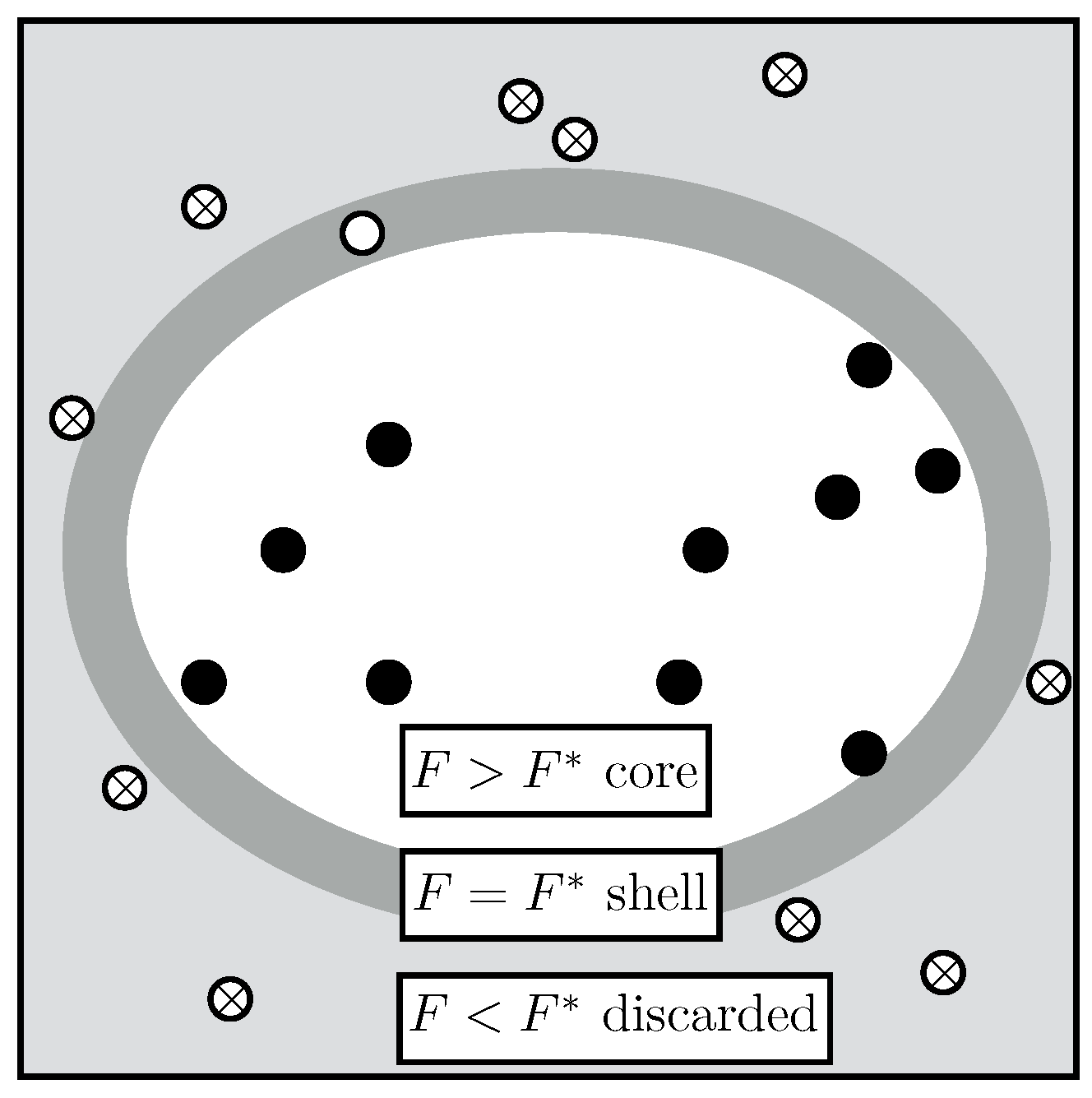
Nested sampling [1,2] counts inwards, estimating volumes statistically from random scatterings of points $\mathbf{x}$, ranked by some quality function $F(\mathbf{x})$ appropriate to the current application (Figure 1). The procedure delves arbitrarily deep by recursively taking proportions of arbitrarily big spaces.

Although suggested by intuition trained in the three dimensions of physical space, geometrical estimation of volume becomes unhelpful in high dimension, where directions tend to be mostly orthogonal, volumes collect around outer boundaries, and spanning the space requires at least as many points as dimensions. Counting is immune to all that.

2. Quantity and Shape

A central use of volume is estimation of the mass (or “quantity”) Q and shape p

$$Q=\int F(\mathbf{x})dV,p(\mathbf{x})=F(\mathbf{x})/Q$$

(1)

of a non-negative density function $F(\mathbf{x})$ defined over a known volume, often thought of as a unit prior measure $V=1$. The information

$$H=\int p(\mathbf{x})logp(\mathbf{x})dV$$

(2)

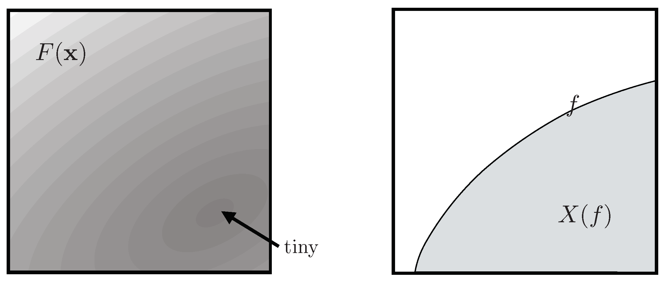
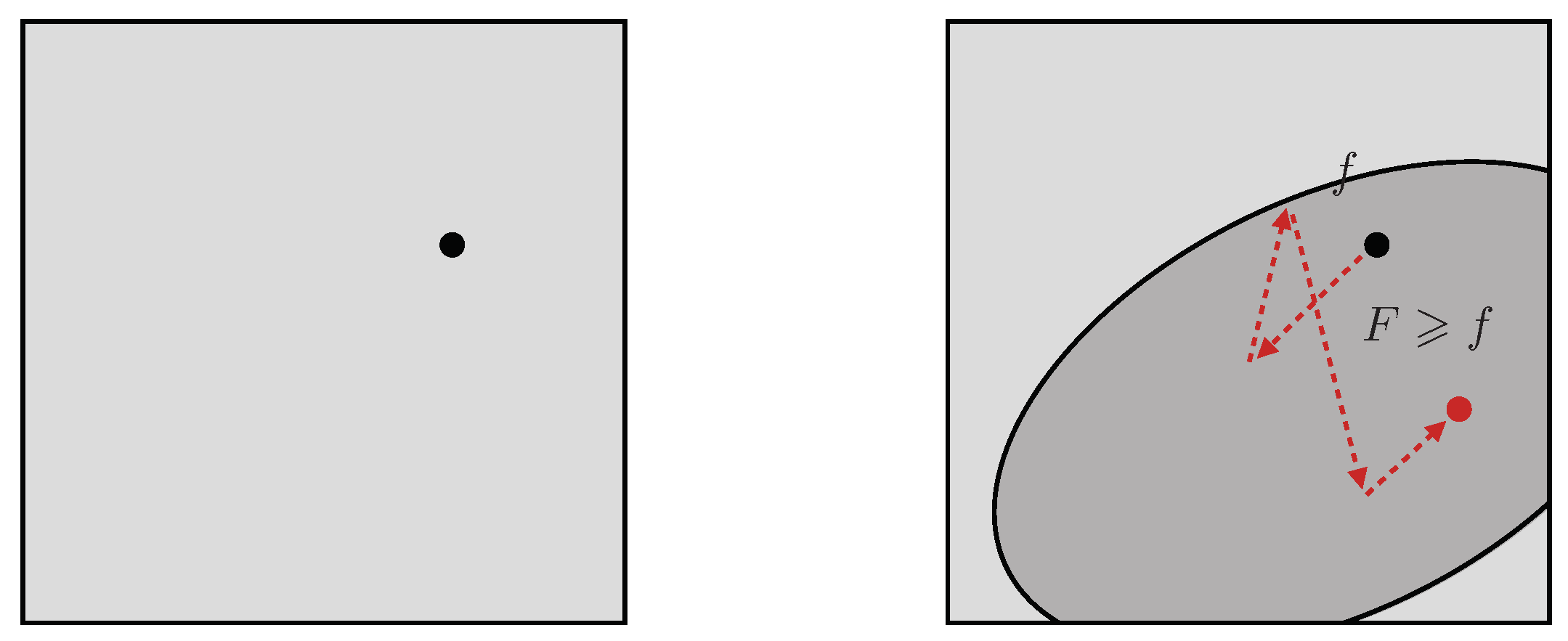
about $\mathbf{x}$ carried by F, measured in nats (logs base e) or bits (base 2), quantifies the corresponding shape. Nested sampling is general but intended for applications where $H\gg 1$ so that the bulk of Q occupies some tiny $O(e^{-H})$ fraction of the original volume (Figure 2 left).

According to fable, mathematicians find a needle in a haystack by iteratively halving the haystack, repeatedly discarding the half that does not contain the needle. Such compression proceeds exponentially, so is linear in H (one bit per step). This neatly outclasses simple point-by-point search, which is proportional to the volume ratio $exp(H)$. Nested sampling operates similarly, with its locations ranked by value F. Volumetric compression controlled by F suggests replacing Q in (1) by the equivalent ($\int ydx=\int xdy$) Lebesgue integral [3]

$$Q={\int }_0^{\infty }X(f)df$$

(3)

where $X(f)={\int }_{F(\mathbf{x})⩾f}dV$ is the volume enclosed by the contour $F(\mathbf{x})=f$ (Figure 2 right). (I am indebted to Ning Xiang in private communication buttressed by [4] for pointing out the Lebesgue connection, which to my embarrassment I had as inventor failed to notice).

X parameterizes a one-dimensional decomposition of quantity Q according to value F. Nested sampling accumulates the quantity and discovers the shape by tracking inwards and upwards, compressing X from the original 1 (complete) towards 0 (empty).

3. Nested Sampling

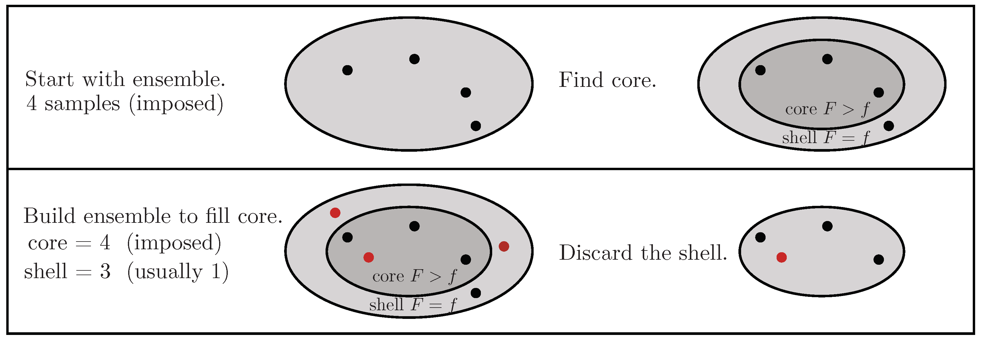
By hypothesis, F is a function accessible pointwise through evaluation at specified locations $\mathbf{x}$, whereas related volumes X have no such easy access. Hence, estimates of Q can realistically only be built from evaluations of F. A priori, we have no knowledge of where good (high value of F) locations $\mathbf{x}$ might be, so we start with a Monte Carlo ensemble of random locations. In any ensemble, there will be one or more locations with the worst (lowest) value f. This outer “shell” $F=f$ surrounds the inner “core” $F>f$ of other locations with better values. For example, the four-object ensemble in Figure 3 (top) has c = 3 objects in the core and s = 1 in the shell.

Compression is achieved by discarding the shell while retaining the core. Actually, any of the ensemble values could be used to divide inner from outer, and the mathematician of the fable would have used the median value. However, compression is smoother, and results are more precise if only the outer shell is discarded. To avoid eroding the ensemble, it is rebuilt with more locations randomly chosen within the current constraint $F⩾f$ until the core $F>f$ contains enough objects that survive. For example, in Figure 3 (bottom), three extra random locations extended the original ensemble until the core built up to the original four objects, with three in the shell that is about to be discarded. For continuous applications, coincident values of F would be vanishingly rare, so a shell would never hold more than one object.

Discarding s (=3) shell objects to leave just the core c (=4) reflects a volume compression ratio around $\frac{c}{c+s}$ (=4/7). This estimate is obtained without any reference to triangulation or geometry or even topology. After discarding the shell, the outermost (lowest) value in the core will define an updated and increased lower limit f, which can seed a subsequent iterate.

With all points distributed uniformly and equivalently, the compression ratio $\gamma$ ($<1$) will have been beta-distributed

$$\gamma \sim \mathtt{Beta}(c,s),\mathrm{explicitly}Pr(\gamma )\propto {\gamma }^{c-1}{(1-\gamma )}^{s-1}.$$

(4)

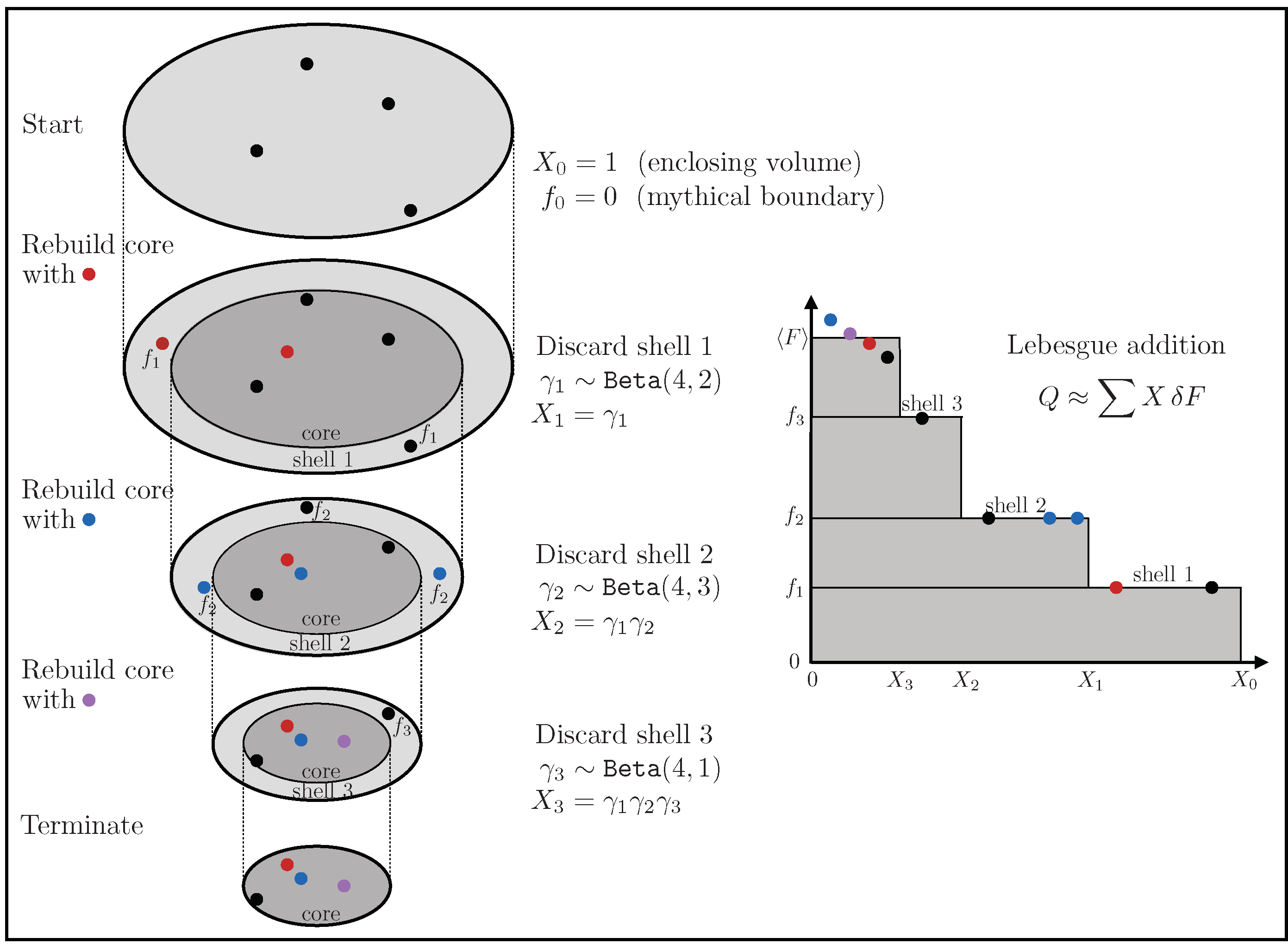
So, when we wish to estimate what $\gamma$ actually was numerically, we can do no better than sample $\mathtt{Beta}(c,s)$, either just once or (preferably) many times. Successive compressions ${\gamma }_1,{\gamma }_2,{\gamma }_3,\dots$ starting from the initial volume $X_0=1$ lead to core volumes (Figure 4 left)

$$X_0=1\stackrel{\times {\gamma }_1}{-----\to }{X}_1={\gamma }_1\stackrel{\times {\gamma }_2}{-----\to }{X}_2={\gamma }_1{\gamma }_2\stackrel{\times {\gamma }_3}{-----\to }{X}_3={\gamma }_1{\gamma }_2{\gamma }_3\stackrel{\times {\gamma }_4}{-----\to }\dots$$

(5)

It is best to keep the shells as thin as possible to maximise the overall compression per sample, which is why we choose to discard just one outermost value at a time. It does not matter if sampling omits intermediate values of F because $\mathtt{Beta}(c,0)$ for an invisibly empty shell ($s=0$) would give $\gamma =1$ so would not contribute to compression.

These multiplicative factors are better accumulated additively as logarithms, for which the mean and standard deviation

$$log\gamma =-\left(\sum _{j=c}^{c+s-1}\frac{1}{j}\right)\pm {\left(\sum _{j=c}^{c+s-1}\frac{1}{j^2}\right)}^{1/2}$$

(6)

imply well-behaved moments of logarithmic compression $log{X}_k$. Conversely, the moments of raw compression $X_k$ rapidly become misleading and unusable. Just as in statistical mechanics where the variable of interest is not raw degeneracy $\Omega$ but the entropy $S=log\Omega$, here it is $logQ$ that matters.

4. Quantity

From the $\gamma$’s, Q is estimated by Lebesgue (3) as

$$Q\approx \underset{\mathrm{nested}\mathrm{sampling}\mathrm{trajectory}}{\underbrace{(f_1-0)X_0+(f_2-f_1)X_1+\cdots +(f_k-f_{k-1})X_{k-1}}}+\underset{\mathrm{termination}}{\underbrace{(\langle F\rangle -f_k)X_k}}$$

(7)

where $\langle F\rangle$ is the terminating mean value (Figure 4 right). The result is a distribution $Pr(Q)$—better represented in view of the large dynamic ranges as $Pr(log Q)$.

5. Approximation

There is no universally valid “best” single-value representative of $Pr(log Q)$, which need not even be unimodal. Neither is there any “unbiassed estimator” for Q or $logQ$. Users who seek a single value may instead plausibly fix each $\gamma$ at its logarithmically mean value (6).

Typically in large applications ($H\gg 1$), the terms in Q rise to a maximum (as increasing F overcomes diminishing volumes X) and then decay (as diminishing volume overcomes limited values of F). Correspondingly, many iterations are needed to scan the volume range. For continuous applications, s will always be 1 so that each $\gamma$ is distributed as $Pr(\gamma )=c{\gamma }^{c-1}$ with logarithmic mean and standard deviation

$$log\gamma =-\frac{1}{c}\pm \frac{1}{c}$$

(8)

Compression by a factor of $e^H$ to the bulk of Q will take about $cH\pm \sqrt{cH}$ such iterates, after which the volume will be estimated with uncertainty $\delta logX\approx \sqrt{H/c}$. The uncertainty will be reflected in Q

$$\delta logQ\approx \sqrt{H/c}$$

(9)

which (under limited computer resources) is minimised by keeping the retained core size c constant.

Of course, that is merely what is anticipated for a typical application. Particular cases may behave worse, and $\delta logQ$ should be estimated statistically if an application has risk of that.

6. Shape

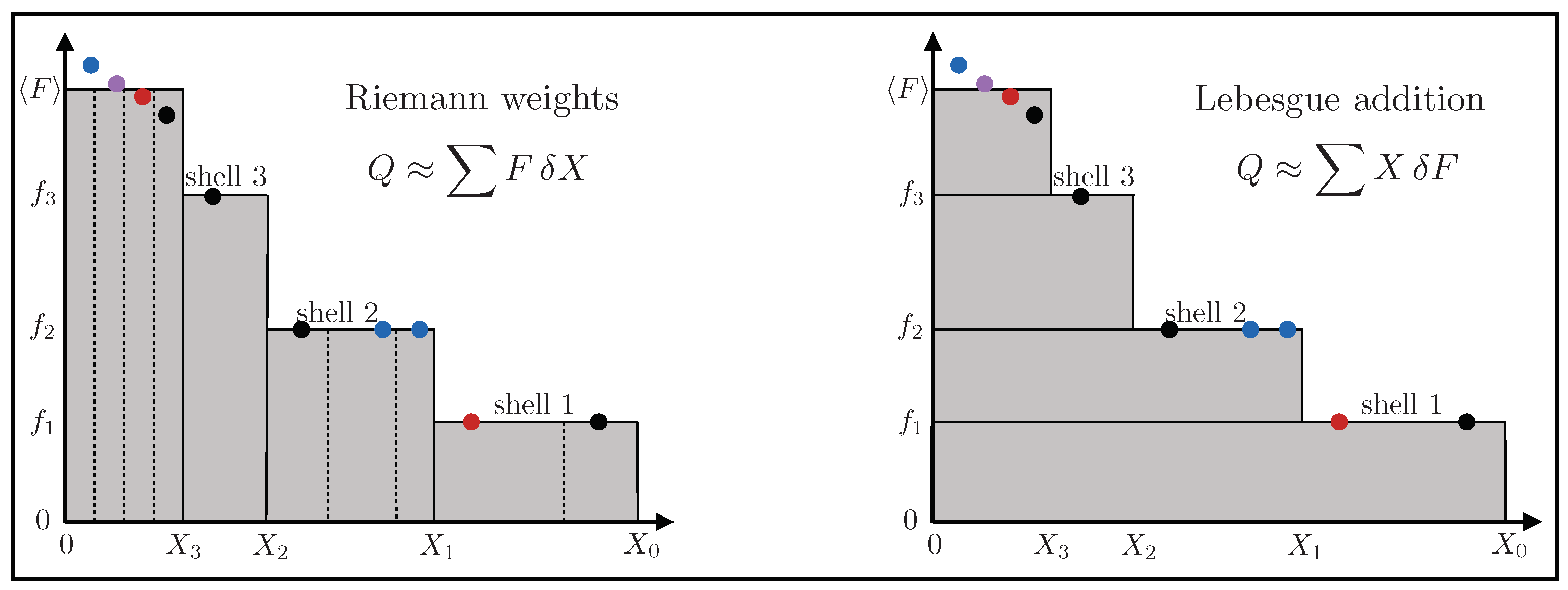
As shells of volume $X_{k-1}-X_k$ are peeled away (Figure 4) to form the nested sampling trajectory, the corresponding value $f_k$ gives a Riemann weight $w_k=(X_{k-1}-X_k)f_k$ (Figure 5 left). That weight can then be randomly assigned among the shell objects to provide a decomposition of quantity according to volume.

Objects drawn randomly in proportion to w then give a usefully compact representation of shape $p(\mathbf{x})$ as a set of equally weighted locations. These introductory locations can be used to seed standard Metropolis MCMC exploration if more samples are wanted.

7. Programming

It may be assumed that the user has, through some such method as importance weighting, already extracted from the original problem whatever structure is analytically available so that the remaining numerical task is reduced as far as reasonably possible. Nested sampling is then to be employed for compressing through the remaining information H.

The following is the minimal skeleton program for nested sampling:

INITIALISE (Figure 6 left)
1:	Set N and allocate $(\mathbf{x},F)$ for N objects	Stored ensemble $0,1,\dots ,N-1$
2:	$X=1$	Initialise volume
3:	$f=0$	Initialise lower bound
4:	$Q=0$	Initialise quantity Q
5:	for $i=0,1,\dots ,N-1$	Initialise ensemble …
6:	$F_i=F({\mathbf{x}}_i$ uniform)	…with random locations ${\mathbf{x}}_i$
ITERATE (Figure 6 right, $\Delta \xi \equiv \xi -{\xi }_{\mathrm{previous}}$)
7:	until (terminate)	Iterate until termination
8:	$f=\mathbf{min}(F_0,F_1,\dots ,F_{N-1})$	Update lower bound f
9:	$\Delta Q=X\times \Delta f$	Update Q (Figure 5 right, lower)
10:	$M=N$	Initial membership = retained storage
11:	for $i=0,1,\dots ,N-1$ randomly	For each stored object, …
12:	while ($F_i$ equals f)	…keep trying again until out of shell
		OUTPUT $({\mathbf{x}}_i,F({\mathbf{x}}_i))$ and M
13:	$F_i=F({\mathbf{x}}_i$ uniform in $F⩾f$)	Replace $({\mathbf{x}}_i,F({\mathbf{x}}_i))$ in $F⩾f$
14:	$\Delta logX=log\gamma (M)$	Compress.
15:	$\Delta M=1$	Increment core+shell membership
TERMINATE
		OUTPUT each $({\mathbf{x}}_i,F({\mathbf{x}}_i))$ and ∅
16:	$f=\mathbf{mean}(F_0,F_1,\dots ,F_{N-1})$	Final ensemble.
17:	$\Delta Q=X\times \Delta f$	Update Q (Figure 5 right, top)

The output forms the nested sampling trajectory, both pre- and post-termination, with each location $\mathbf{x}$ representing its shell of volume $\Delta X$ having values at or around $F(\mathbf{x})$, and compression defined by M with core size N. The compression ratio $\gamma (M)$ in line 14 can be either the probabilistic estimate $\mathtt{Beta}(M,1)$ (4) or the approximating logarithmic mean value $e^{-1/M}$ (8).

The program’s overt purpose is to accumulate the quantity Q according to Lebesgue summation (7). This accumulation is parasitic upon nested exploration which is driven only by ranking of quality, so that arbitrary monotonic quantities $\Theta =\int X(f)d\theta (f)$ could be accumulated consistently at the same time.

Apart from the procedure for evaluating $F(\mathbf{x})$, the program requires three inputs from the user.

A: 

A Monte Carlo procedure for a random $\mathbf{x}$ uniformly distributed over the original unit volume (Figure 6 left), used in line 6.

B: 

A procedure for generating a new $\mathbf{x}$ uniformly distributed within the current constraint $F(\mathbf{x})⩾f$, used in line 13. In practice, this will be a Markov chain (MCMC) procedure seeded at a random member of the current ensemble and exploring the constrained volume with moves obeying detailed balance (Figure 6 right). Note that these moves are not modulated by F, except that destinations below f are prohibited. Geometrical properties of an application may assist construction of the MCMC procedure, as when ellipsoidal domains are constructed around the walkers in suitably smooth applications in suitably restricted dimension ([5] etc.), but nested sampling itself is not dependent on geometry or topology or continuity or differentiability or convenient shapes. It is for the user to program a suitable procedure for the application in hand. Or fail in the attempt.

C: 

A termination criterion, needed in line 7. There is no universally valid criterion because numerical experimentation alone can never exclude the possibility of high values in unreached locations which could render termination premature. Your author’s default criterion is to terminate when H, which can be accumulated through $\Delta (QH+QlogQ)=X\Delta (flogf)$, appears to have stopped increasing significantly, indicating that most of the relevant structure has likely been found.

Lines 1–6 of the program are straightforward initialisation of a random N-object ensemble.

Lines 7–15 are the iterative loop. On entry, the ensemble has N core objects. The bounding (lowest) value f is appropriately increased (line 8) and Q updated (line 9). At least one object then lies on the new boundary with $F=f$ (the new shell), with the others in the diminished core $F>f$. The aim is to add new randomly located objects until the core has again built up to N, following which the shell can be discarded (or, more usefully, output as the trajectory).

Whenever a shell object is discovered within the N-object stored ensemble (Lines 11 and 12), it is written out to the trajectory to make room for a new random location. When that new location is generated (Line 13), it is included in the extended membership M (line 15). Meanwhile, the corresponding 1-in-M contribution to compression is incorporated in Line 14. This loop (Lines 11 to 15) ends when the new location falls into the now-more-populated core. The iterate ends when every stored object is in the core, with every shell object having been written to the trajectory ($c=N$, $s=M-N$).

Compression could be programmed using a single ratio $\gamma =\mathtt{Beta}(c,s)$ (Equation (4)) just before Line 9 to discard the whole shell in one go. However, it is better to use the individual steps shown in Line 13. That is equivalent to grouped compression, and $\mathtt{Beta}(M,1)$ is quick to compute.

$$\mathtt{Beta}(c,s)=\prod _{k=c}^{c+s-1}\mathtt{Beta}(k,1),\mathtt{Beta}(k,1)={\left(\mathtt{Uniform}(\mathtt{0},\mathtt{1})\right)}^{1/k}.$$

(10)

Lastly, if the program has been properly terminated with the bulk of the structure found, the contribution of the final ensemble (Lines 16 to 17) will be negligible and could be omitted.

Because of the dynamic range inherent in large problems, the skeleton program as written is susceptible to computer over/underflow. Therefore any useful implementation should store $X,F,Q,w$ as logarithms.

A professional refinement is to track several chains of Beta-distributed compressions in line 14 to obtain the distribution of Q. Production of a nested sampling trajectory $\{\mathbf{x},F\}$ was statistical, so its interpretation ought also to be statistical.

8. Convergence

There has been a view in the community [6,7] that interest lies in, and convergence should be proved for, Q rather than $logQ$. That view is a relic of bygone concentration on small problems—misleading nowadays because the extremely heavy-tailed distribution of Q in applications of appreciable size requires excessive resources to decrease $\delta Q$ below Q. As mentioned below (6), it is variation in $logQ$ that matters, even if that residual uncertainty allows orders of magnitude of uncertainty in Q.

In most practical applications, a run can be continued until compression has scanned through most of the posterior distribution, as indicated by flattening off of H as it rises toward its presumed final value. In such cases, rms convergence of $logQ$ proceeds as the usual statistical inverse-square-root $O(n^{-1/2})$, where $n\gtrsim cH$ is the number of iterative steps as in (9). That fact can be demonstrated by observing that the number of iterates n required to compress volume from 1 to X is a Poisson distribution with mean $-clogX$, which consequently has inverse-square-root uncertainty. The compression $-logX$ inferred from n is then exponential with mean $n/c$, with that same inverse-square-root uncertainty. The overall effect is then inverse square root as stated.

Incidentally, the behaviour of nested sampling depends on the prior-to-posterior information H, which can be unrelated to dimension. Dimension, which is a geometrical construction, is not part of nested sampling. Applications need not even have a dimension.

Exceptionally, there may be a localised but important quality peak hiding beyond termination and yielding substantial or even dominant termination error. It was shown in [8] that termination error is controllable if H can be bounded above. Resources can then be adjusted to yield convergence as $O(n^{-1/4})$. Of course, the information H is always bounded in any practical application: the question would be how to define a convincing upper limit.

Those analyses assumed that the ensemble size was held constant, with implicitly unit shells $s=1$ surrounding a constant core size c. But, in discrete applications, plateaus of constant quality F may necessitate larger shells, which require extra resources to traverse. Indeed, Mother Nature can supply arbitrarily challenging problems, to which we have no general answer.

Ultimately, finding a 1-in-$e^{-H}$ posterior domain may require $e^H$ exploratory samples, thus defeating the enterprise. Numerical exploration will never be able to find a flagpole in the Atlantic Ocean.

References

- Skilling, J. Nested Sampling. In Bayesian Inference and Maximum Entropy Methods in Science and Engineering, Garching, Germany 2004; Fischer, R., Dose, V., Preuss, R., von Toussaint, U., Eds.; AIP Publishing LLC: New York, NY, USA, 2004; Volume 735, pp. 395–405. [Google Scholar] [CrossRef]
- Skilling, J. Nested sampling for general Bayesian computation. Bayesian Anal. 2006, 1, 833–859. [Google Scholar] [CrossRef]
- Lebesgue, H. Leçons Sur l’intégration et la Recherche des Fonctions Primitive; Gauthier-Villars: Paris, France, 1904. [Google Scholar]
- Jasa, T.; Xiang, N. Using Nested Sampling in the Analysis of Multi-Rate Sound Energy Decay in Acoustically Coupled Rooms. In Bayesian Inference and Maximum Entropy Methods in Science and Engineering; Knuth, K.H., Abbas, A.E., Morris, R.D., Castle, J.P., Eds.; AIP Publishing LLC: New York, NY, USA, 2005; Volume 803, pp. 189–196. [Google Scholar] [CrossRef]
- Mukherjee, P.; Parkinson, D.; Liddle, A.R. A nested sampling algorithm for cosmological model selection. Astrophys. J. Lett. 2006, 638, L51. [Google Scholar] [CrossRef]
- Evans, M.J. Discussion of “Nested Sampling for Bayesian Computations”. In Bayesian Statistics 8; Bernardo, J.M., Bayarri, M.J., Berger, J.O., Dawid, A.P., Heckerman, D., Smith, A.F.M., West, M., Eds.; Oxford University Press: Oxford, UK, 2007; pp. 507–512. [Google Scholar]
- Chopin, N.; Robert, C.P. Properties of nested sampling. Biometrika 2010, 97, 741–755. [Google Scholar] [CrossRef]
- Skilling, J. Nested sampling’s convergence. In Proceedings of the Bayesian Inference and Maximum Entropy Methods in Science and Engineering, Oxford, MS, USA, 5–10 July 2009; Goggans, P.M., Chan, C.Y., Eds.; AIP Publishing LLC: New York, NY, USA, 2009; Volume 1193, pp. 277–291. [Google Scholar]
Figure 1.
Sample ranked r out of n encloses about of the volume.
Figure 2.
(left) unit volume V modulated by F; (right) volume covering .
Figure 3.
Nested sampling iterate with ensemble size 4.
Figure 4.
Nested sampling trajectory.
Figure 5.
Riemann and Lebesgue.
Figure 6.
(left) set prior object by MC; (right) generate new object by MCMC.
Disclaimer/Publisher’s Note: The statements, opinions and data contained in all publications are solely those of the individual author(s) and contributor(s) and not of MDPI and/or the editor(s). MDPI and/or the editor(s) disclaim responsibility for any injury to people or property resulting from any ideas, methods, instructions or products referred to in the content. |
© 2024 by the author. Licensee MDPI, Basel, Switzerland. This article is an open access article distributed under the terms and conditions of the Creative Commons Attribution (CC BY) license (https://creativecommons.org/licenses/by/4.0/).
Share and Cite
MDPI and ACS Style
Skilling, J. Nested Sampling—The Idea. Phys. Sci. Forum 2023, 9, 22. https://doi.org/10.3390/psf2023009022
AMA Style
Skilling J. Nested Sampling—The Idea. Physical Sciences Forum. 2023; 9(1):22. https://doi.org/10.3390/psf2023009022
Chicago/Turabian StyleSkilling, John. 2023. "Nested Sampling—The Idea" Physical Sciences Forum 9, no. 1: 22. https://doi.org/10.3390/psf2023009022