Proceeding Paper

Physics-Consistency Condition for Infinite Neural Networks and Experimental Characterization †

Institute of Theoretical Physics-Computational Physics, Graz University of Technology, Petersgasse 16, 8010 Graz, Austria
*
Author to whom correspondence should be addressed.
Presented at the 42nd International Workshop on Bayesian Inference and Maximum Entropy Methods in Science and Engineering, Garching, Germany, 3–7 July 2023.
Phys. Sci. Forum 2023, 9(1), 15; https://doi.org/10.3390/psf2023009015
Published: 4 December 2023

Abstract

:
It has previously been shown that prior physics knowledge can be incorporated into the structure of an artificial neural network via neural activation functions based on (i) the correspondence under the infinite-width limit between neural networks and Gaussian processes if the central limit theorem holds and (ii) the construction of physics-consistent Gaussian process kernels, i.e., specialized covariance functions that ensure that the Gaussian process fulfills a priori some linear (differential) equation. Such regression models can be useful in many-query problems, e.g., inverse problems, uncertainty quantification or optimization, when a single forward solution or likelihood evaluation is costly. Based on a small set of training data, the learned model or “surrogate” can then be used as a fast approximator. The bottleneck is then for the surrogate to also learn efficiently and effectively from small data sets while at the same time ensuring physically consistent predictions. Based on this, we will further explore the properties of so-constructed neural networks. In particular, we will characterize (i) generalization behavior and (ii) the approximation quality or Gaussianity as a function of network width and discuss (iii) extensions from shallow to deep NNs.

1. Introduction

The impressive achievements of neural networks (NNs) in computer science have sparked a growing interest also in physics and scientific computing. Here, we explore their utilization as surrogate models in computationally intensive tasks like simulation-based optimization or uncertainty quantification [1,2]. For this, the surrogates’ predictions should be consistent with physics, which typically cannot be achieved with data alone as such models often generalize poorly, i.e., they learn the physics implicitly and well only in regimes where (enough) data are available.
Here, we pursue a previously proposed approach [3] as follows: (i) linear differential equations can be inherently integrated into a Gaussian process (GP) model by carefully selecting the covariance function or kernel [4,5,6,7,8]. The GP defined by the so-constructed kernel may be referred to as a “physics-consistent GP” [6]. (ii) Neal [9] established that Bayesian NNs converge toward a GP in an infinite-width limit using the central limit theorem. By combining these two insights, we infer that at least some laws of physics can also be a priori embedded into a suitable infinite NN model by choosing neural architecture and activation functions in alignment with the corresponding GP’s kernel, i.e., the corresponding infinite NN has the same physics-consistency property as the physics-consistent GP. Note that this approach fundamentally differs from “physics-informed” learning machines [10], where the residual of the equation (of the physical law) is included into the loss function independent of NN architecture. Departing from the foundations introduced in [3], we here consider generalization outside of the training data regime, and Gaussianity, i.e., convergence of the infinite-width limit approximation.

2. Background

This section provides a concise overview of the relevant literature on Gaussian processes (GPs), neural networks (NNs), and the infinite-width correspondence between the two. Additionally, related works on physically inspired GPs and NNs are discussed.

2.1. Physics-Consistent Gaussian Processes

Gaussian process regression, also known as “Kriging”, has been extensively studied for several decades [11]. GPs have become one of the most popular classes of machine learning [12] and Bayesian models [13], and found wide application in the field of “Uncertainty Quantification” [14,15]. The defining element of a Gaussian process is its covariance function, also referred to as the kernel. Consequently, significant efforts have been dedicated to the design and selection of appropriate kernel functions [16].
As a matter of fact, a linear (differential) operator applied to a GP results in another GP with a modified kernel [5,6,7,17]. This allows one to derive a “physics-consistency condition” for the kernel, allowing the construction of kernels to define a GP that satisfies physical laws expressed in terms of said differential equations a priori, i.e., before training. Examples include divergence-free fields [18] and the Helmholtz equation [6]. More general linear constraints and boundary conditions can be considered in an analogous manner [17,19,20,21]. Note that it is also possible to construct physics-based or “weakly” physics-informed GPs through training [22] given some (non necessarily physical) base kernel, or through Green’s functions [23,24].
While this approach was generally believed to be limited to linear equations, it has recently been extended even toward non-linear partial differential equations (PDEs) [25].

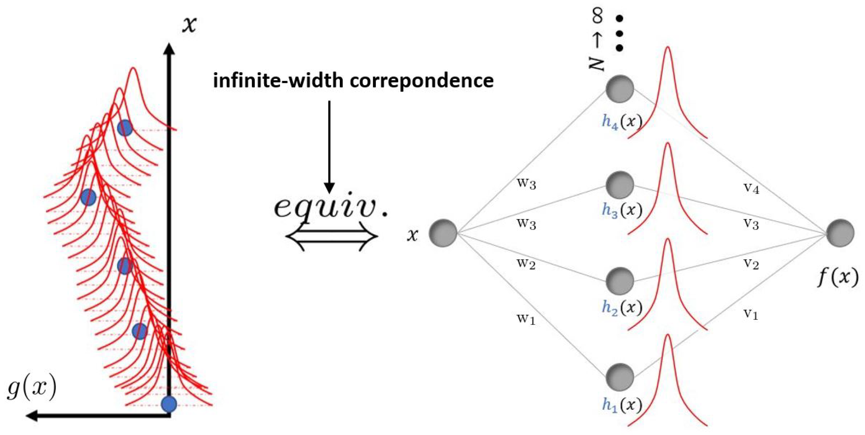
2.2. Infinite Neural Networks

Neural networks (NNs) are arguably one of the most popular classes of machine learning models. Similar to GPs and kernels, the design and selection of activation functions play a crucial role in NNs. Numerous activation functions have been proposed [26,27], but few principled approaches are known on how to choose an appropriate neural activation.
The infinite-width correspondence relates to the fact that Bayesian NNs converge toward a GP under the infinite-width limit [9]. This infinite-width correspondence has been used to compute kernels for GPs corresponding to specific neural activations and architectures [28,29,30,31,32], which may be regarded as a form of the “kernel trick”. However, the inverse approach, i.e., computing activations from kernels, has received little attention. Here, we aim to take this route due to the beneficial circumstance that we can make GPs physics-consistent. Note that the term “physics-informed neural network” relates to training based on a physics-loss term composed of the differential equation residual, and was popularized by Raissi et al. [33], although the idea was around earlier [34,35].
Quite importantly, it has recently been shown that a very large class of NN architectures converge toward a GP [36], including deep NNs [29], convolutional NNs [37], recurrent NNs [38] and transformers [39]. Furthermore, the infinite-width limit provides valuable insight into the training dynamics of NNs as well [40]. Note that random Fourier features [41] also share the underlying mechanism of the central limit theorem. As for interactions arising from the breaking of CLT through either a finite number of neurons or non-independence of neurons, i.e., the emergence of a non-Gaussian field, see [42].

3. Infinite Neural Networks Converging to Physics-Consistent Gaussian Processes

In this section, we give a brief review of the notions introduced previously in [3]. We introduce two sets of functions (function spaces) V , W : X Y R Q . From the first set V, we denote two particular elements (i.e., functions from this space) as g ( x ) V , x g ( x ) and f ( x ) V , x f ( x ) , x X R D , where D , Q denote the input/output dimension. We will later see that GPs are distributions for functions; hence, we need sets of functions accordingly. We aim to learn these functions from data related to some physical law expressed in terms of a linear operator O ^ : V W , O ^ f ( x ) f ˜ ( x ) . In words, an operator maps a function from the set (function space) V to another function from the set (function space) W. Linearity requires O ^ ( α · f + β · g ) = α · O ^ f + β · O ^ g for some constants α , β R . Let the physical law be expressed in the form O ^ f ( x ) = 0 , where, from now on, we omit the ∘-sign for simpler notation, e.g., if O ^ were the D-dimensional Laplace-operator O ^ 2 : = k = 1 D 2 x k 2 , x k denoting the k t h element of D-dimensional vector x = ( x 1 , , x D ) T , then V would be at least the set of (continuous) functions twice-differentiable and O ^ : C 2 ( X ) C 0 ( X ) C 2 ( X ) , i.e., W V .
In the following, g will denote a GP and f will denote an NN.

3.1. Physics-Consistent Gaussian Processes

We will introduce GPs along the lines of [7]. A GP is a distribution on the set of functions R D R Q such that the function values g ( x ( 1 ) ) , , g ( x ( n ) ) at x ( i ) R D have a joint Gaussian distribution. Note the consistent marginalization property that follows from this definition. The distribution is specified by a mean function μ : R D R Q : x g ( x ) and a positive semi-definite covariance function k : R D R D R 0 Q × Q : ( x , x ) g ( x ) μ ( x ) g ( x ) μ ( x ) T , where · denotes expectations. k is also known as kernel, and the common notation is g ( x ) GP μ ( x ) , k ( x , x ) . For simplicity, we assume g to be a zero-mean GP,
g ( x ) GP 0 , k ( x , x )
We further require that g be consistent with a physical law expressed in terms of a linear differential operator O ^ x , i.e., differential with regard to x, i.e., that it admits the following equation:
O ^ x g ( x ) = 0 ,
In other words, we use a GP as an ansatz for solving Equation (2). As mentioned before, this is a differential operator defining a differential equation. Then, due to the linearity of O ^ ,
O ^ x g ( x ) GP 0 , O ^ x O ^ x k ( x , x )
where † denotes the adjoint, acting on the second argument of the kernel function x . We have introduced the subscript x to clarify which argument of the kernel the differential operator is acting on. At this point, we restrict ourselves to linear operators, but recent extensions to non-linear differential PDEs have been fairly successfully [25]. The above relationship can be used to formulate a number of equivalent physics-consistency conditions for the GP (or its kernel, respectively), e.g., from [5]:
O ^ x O ^ x k ( x , x ) | x = x = ! 0 .
The solution for k in Equation (4) then defines a GP that satisfies Equation (3) a priori, i.e., before training. In other words, these physics-consistency conditions can be used to find and design physics-consistent kernels. For this, Mercer’s theorem can be especially useful, in that it states that a kernel function (i.e., an element from a reproducing kernel Hilbert space) can always be expressed in terms of a set of basis functions { ϕ i } and vice versa [43]. Formally, this means that
k ( x , x ) = lim P i , j P ϕ i ( x ) M i j ϕ j ( x )
with a suitable prior covariance matrix M for the function weights. Those basis functions could, e.g., be constructed from Green’s functions as proposed by [6]. Exploiting linearity and requiring uniform convergence, the substitution of Equation (5) into Equation (4) would lead the operators to act on the basis functions in the sum directly. Note that [7] introduced a symbolic, algebraic algorithm program for constructing such kernels.

3.2. Infinite Neural Networks

Let us now consider an NN f with a single hidden layer with N neurons with non-linear but bounded activation functions h,
f ( x ) = k = 1 N v k h k w k · x + b k ,
where the index k = 1 , , N sums over the N neurons in the single hidden layer. w k are the input-to-latent weight matrices, b are bias terms and v k are the latent-to-output weights. Under the infinite-width limit, N , Equation (6) converges to a Gaussian process, i.e., a Gaussian distribution x , using the central limit theorem if the activation functions h k are bounded and weights and biases are i.i.d. [9]. Figure 1 shows an illustration of the correspondence between GPs and infinite NNs.
The same finding holds for a considerably larger class of models [36]. Then, the NN converges to a GP with kernel k ( x , x ) = f ( x ) f ( x ) , i.e., the covariance of NN predictions must satisfy the covariance of the GP, which is a sensible requirement. This gives rise to the following condition for equivalence between a certain GP and a certain NN:
k ( x , x ) = ! f ( x ) f ( x ) lim N k = 1 N k = 1 N v k v k h k ( w k x + b k ) h k ( w k x + b k ) p ( θ ) d V θ
where we used the linearity of the expectation and p ( θ ) is the probability density function of the weights and biases θ = { v , w , b } . Note that we exchanged limit and integration, which is (typically) permissible if convergence is uniform and the limit function is integrable [44]. This integral can be solved numerically and, in some cases, analytically [28]. Note that Equation (7) is essentially determined by the covariance of the activations.

3.3. Physics-Consistency Condition for Neural Networks

We could now take the route of finding a physics-consistent kernel k on the left-hand side of Equation (7) and then try to find “physics-consistent” activations, i.e., activations such that the infinite NN becomes a physics-consistent GP. This approach may be regarded as an “inverse kernel trick”, especially if the Mercer representation is used.
An alternative route would be to find physics-consistent activations directly. Substituting the NN-GP consistency condition Equation (7) into the physics-consistency condition for the GP Equation (4) (or variants thereof) allows us to formulate a physics-consistency condition for the NN directly. Reciting uniform convergence and integrable limits as above used for Equation (7) [44], we switch the order of limit, expectation and differentiation:
lim N p ( θ ) d V θ k , k = 1 N v k v k O ^ h k ( w k x + b k ) · O ^ h k ( w k x + b k ) | x = x = ! 0 .
where the chain rule has to be applied, giving rise to differentiated activations x [ O ^ h k ] ( x ) applied to their original argument ( w k x + b k ) , where, if h k ( x ) V , then [ O ^ h k ] W . This gives rise to the problem of finding pairs of probability density functions p ( θ ) and activations h such that the physics-consistency condition for the NN Equation (8) is satisfied. This implies that the choice of activation and prior cannot be simply treated separately. The choice of prior p ( θ ) and activation h is then reminiscent of the choice of the prior covariance matrix M and basis functions ϕ in the Mercer representation of the GP kernel in Equation (5).
Through equating Equation (8) l.h.s. with the kernel’s Mercer representation, Equation (5), and recalling that Green’s functions can admit kernels (i.e., applying the kernel trick to Green’s functions), it is easy to see through the choices M i j = σ v i δ i j , Gaussian priors and the limit p ( w k ) = lim σ w k 0 N ( 0 , σ w k 2 Σ ) (where Σ is diagonal) that h ϕ . This means that the activations become the Green’s functions [3].

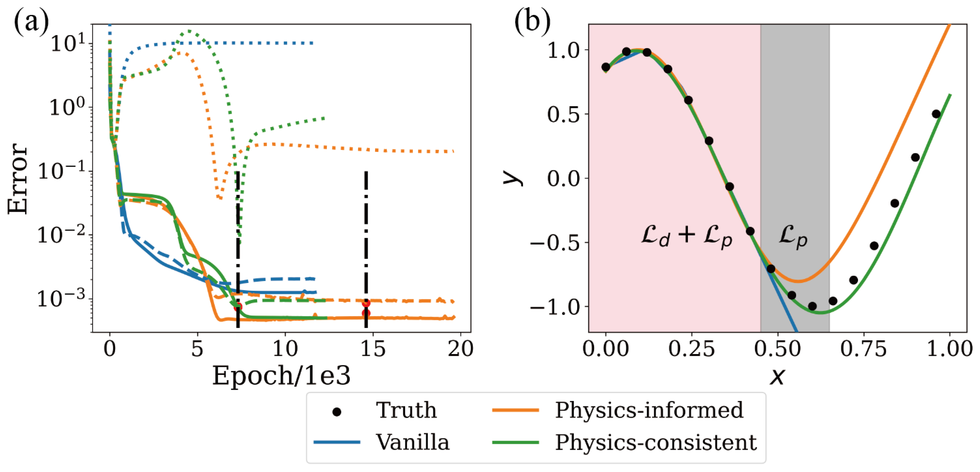
3.4. Training and Regularization with Physics-Information

Given pairs of input–output data D = { x ( d ) , y ( d ) } d = 1 N d , where y ( d ) = f ( x ( d ) ) + ε are noisy observations with noise ε , we ought to choose an optimization criterion or loss function for the learning, e.g., here,
θ * = arg min θ d = 1 N d y ( d ) f ( x ( d ) ) 2 + λ p = 1 N p O ^ x f ( x ) | x = x ( p ) ,
which essentially consists of the likelihood and a prior defined via the residual of Equation (3). The last term denotes the differential to be applied to f and then evaluated at pivot points x = x ( p ) that may be distinct from the data points x ( d ) . In more detail, for the second term (the “prior”), a network f is substituted as an ansatz function into Equation (3) and evaluated at pivot points (or sometimes called collocation points) x ( p ) . This evaluation generally yields non-zero values for a generic NN (as opposed to the zero right-hand side in Equation (3), i.e., the equation at this point is not actually satisfied). The sum of these (absolute) values may be called the residual. In the physics-informed training approach, this residual is to be minimized by adjusting the function parameters (in an NN, the weights and biases). This minimization can be performed conjointly with minimizing the data misfit (i.e., the first term in Equation (9)), where the trade-off between the physics-residual and the data misfit term is controlled by a tunable regularization parameter λ . The choice of λ and the set { x ( p ) } p = 1 N p is generally non-trivial [45].

4. Experiments

4.1. Generalization

We consider a Helmholtz equation
( 2 c 2 ) f ( x ) = 0
where c = 6.0 is a constant parameter related to the wavenumber. In the one-dimensional case, the solution to this equation is a sinusoidal function. The physics-consistent GP kernel for this physical law in 1D has the form k ( x , x ) = cos α ( x x ) [46]. As derived in [3], one particular activation that defines an infinite NN with the same physics-consistent covariance is a sinusoidal activation function, h ( · ) : = sin ( · ) .
We used the function y = A sin ( ω x + ϕ ) to generate the training data. A noise of normal distribution N ( 0 , 0 . 04 2 ) was added to the training sets. Next, we tried to learn an NN function f ( x ) from this data, and compared the performance of three networks: all three networks are single-layer with the structure introduced before with N = 100 neurons in the hidden layer. We denote as “vanilla” a simple NN with an ReLU ( · ) activation, and training with L 2 -loss. We denote as “physics-informed” the same network where the training is additionally regularized through a physics-loss term as in Equation (9). For the physics-informed neural network, the loss function specifically is L = L d + L p = | y y ^ | 2 + λ | 2 y + c 2 y | . Note that in the physics-consistent NN, there are no training difficulties due to higher-order derivatives and the training is as straightforward and fast as with the vanilla NN.
Note the distinction between training error, validation error and testing error. The training error is the prediction error on the training sets. Additional validation sets are used for early stopping to avoid overfitting, where training is stopped if there is no improvement in validation errors for a number of epochs. The validation sets are distributed within the same range/domain as the training sets, and test sets are distributed in a different range. The test sets are typically used to investigate the generalization behavior of an NN.
One reason for the wide-spread popularity of physics-informed NNs (PINNs) is that they typically generalize better than NNs trained on the data alone. PINNs achieve this by introducing a weak constraint that penalizes un-physical behavior. In our physics-consistent approach, in contrast, we enforce a hard constraint instead. In particular, this avoids the inconsistency of the multiple training objectives or the Pareto front as discussed in [47].
We compare the generalization behavior of the three NNs in Figure 2.

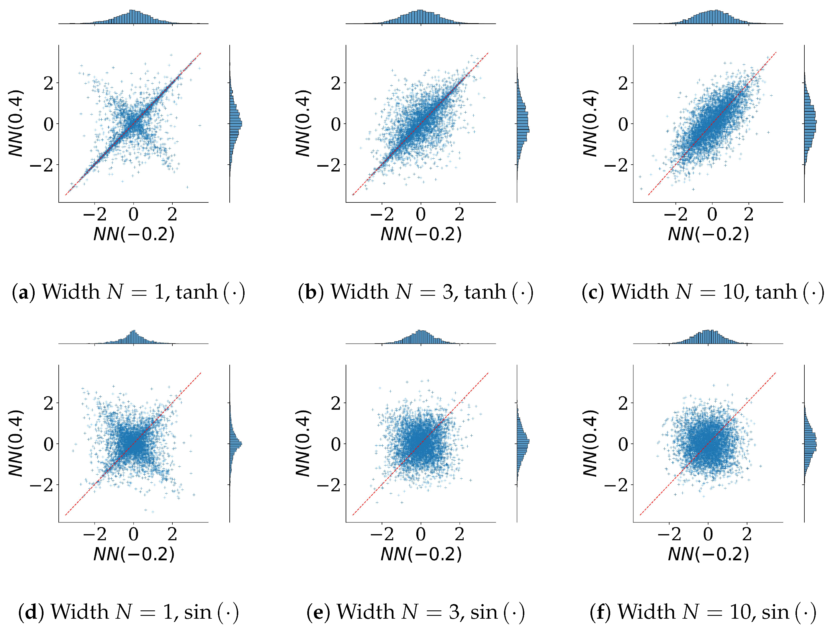
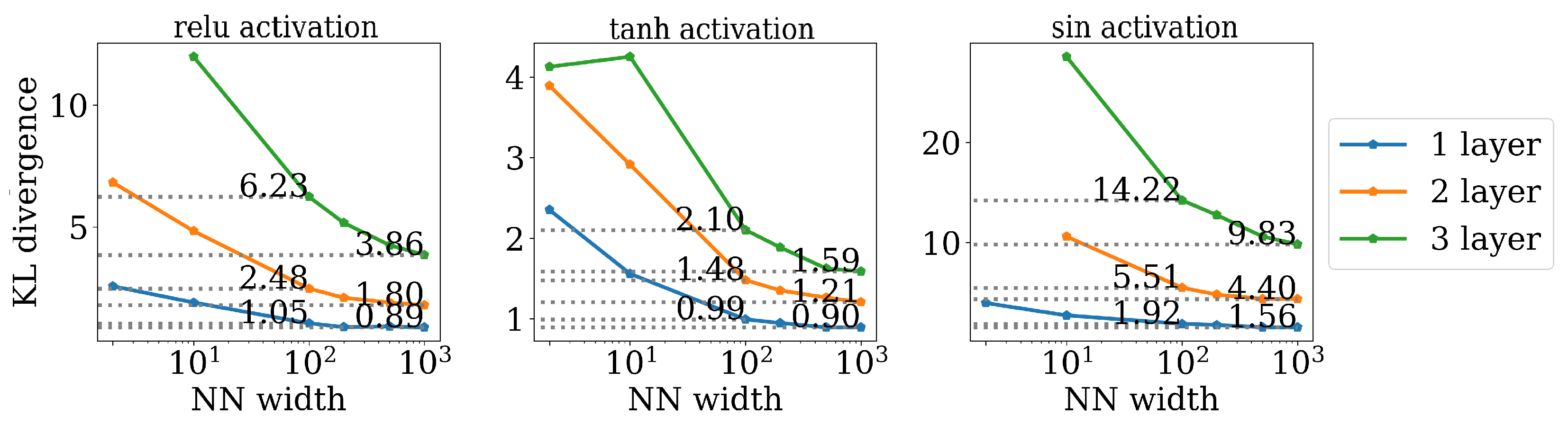
4.2. Convergence to Gaussian as a Function of Network Width

The Gaussianity of an NN is only exact under the infinite-width limit, whereas, on a computer, NNs are always finite. This begs the question of how good the approximation is as a function of NN width, or how fast the NN converges to a GP. Here, we use a single-hidden-layer neural network with prior distributions all i.i.d. normal with zero-mean. The variances are σ w = 5 , σ b = 5 , σ v = 1 , σ a = 0.1 .
For pedagogical illustration, we show scatter plots in Figure 3 of predictions collected from simple Monte Carlo samples from the prior on the weights and biases, p ( θ ) similar to [9] with a single-layer NN and tanh ( · ) -activations. N N ( 0.2 ) and N N ( 0.4 ) denote the outputs of the network corresponding to the inputs x = 0.2 and x = 0.4 , respectively.
The NN’s limit kernel is defined by Equation (7). For some NNs, this kernel can be computed analytically, while more often it has to be computed numerically, e.g., through Monte Carlo integration. For a single-layer NN with ReLU-activation, we compare the analytical kernel to the estimated kernel in Figure 4, which shows that such estimates can converge quickly and easily with only few neurons and samples.
This, however, is only an estimate of the second moments, and does not tell “how Gaussian” the distribution itself is. One suitable measure for this would be the Kullback–Leibler divergence, measuring the (dis-)similarity between two probability distributions. By defining a Gaussian distribution Q = N ( 0 , K Q ) defined by the computed or estimated covariance matrix K, e.g., from Figure 4, the Kullback–Leibler divergence allows us to measure the dissimilarity between the distribution of NN predictions P ( f ( x ) , i.e., the histograms of NN realizations collected from prior samples fed through the NN as in the scatter plots in Figure 3, and the (Gaussian) limit distribution Q. Note that alternative measures would be possible, such as the Wasserstein distance.
The Kullback–Leibler divergence is defined as:
D K L ( P Q ) = x X P ( f ) log P ( f ) Q ( f )
which can be estimated, e.g., through Monte Carlo. We plot the KL-divergence between the finite NN and its infinite-limit Gaussian as a function of the finite network’s width in Figure 5. The result confirms the intuition from Figure 3, and the finite NN behaves similar to a Gaussian already with just 10 2 neurons.

5. Conclusions

We have derived a physics-consistency condition for NNs by exploiting the physics-consistency condition for GPs along with infinite NNs converging to GPs using the central limit theorem. We quantify experimentally that finite NNs with only order ∼10 2 neurons already behave like GPs, i.e., that the approximation is sensible. We further show that engineering NNs to be physics-consistent can have advantages over both purely data-driven approaches and physics-based approaches with a similar intent, e.g., PINNs, in terms of convergence rate and generalization.

Author Contributions

Conceptualization, S.R.; methodology, S.R.; software, S.G.; validation, S.R. and S.G.; formal analysis, S.R.; investigation, S.R. and S.G.; resources, S.R.; data curation, N/A; writing—original draft preparation, S.R.; writing—review and editing, S.R. and S.G.; visualization, S.G. and S.R.; supervision, S.R.; project administration, S.R.; funding acquisition, S.R. All authors have read and agreed to the published version of the manuscript.

Funding

The authors gratefully acknowledge funding by UFO—Unkonventionelle Forschung of Das Land Steiermark (Styrian Government), Abt. 12 Referat für Wissenschaft & Forschung, PN32.

Institutional Review Board Statement

Not applicable.

Informed Consent Statement

Not applicable.

Data Availability Statement

All information is contained in the manuscript. Codes are available at https://github.com/guanshaoheng/gaussian_nn_tugraz (accessed on 1 July 2023).

Acknowledgments

S.R. carried out parts of the research during a visit at the Munich Institute for Astro-, Particle and BioPhysics (MIAPbP), funded by the Deutsche Forschungsgemeinschaft (DFG, German Research Foundation), Germany’s Excellence Strategy—EXC-2094—390783311.

Conflicts of Interest

The authors declare no conflict of interest.

References

  1. Ranftl, S.; von der Linden, W. Bayesian Surrogate Analysis and Uncertainty Propagation. Phys. Sci. Forum 2021, 3, 6. [Google Scholar] [CrossRef]
  2. Ranftl, S.; Rolf-Pissarczyk, M.; Wolkerstorfer, G.; Pepe, A.; Egger, J.; von der Linden, W.; Holzapfel, G.A. Stochastic modeling of inhomogeneities in the aortic wall and uncertainty quantification using a Bayesian encoder–decoder surrogate. Comput. Methods Appl. Mech. Eng. 2022, 401, 115594. [Google Scholar] [CrossRef]
  3. Ranftl, S. A Connection between Probability, Physics and Neural Networks. Phys. Sci. Forum 2022, 5, 11. [Google Scholar] [CrossRef]
  4. Dong, A. Kriging Variables that Satisfy the Partial Differential Equation ΔZ = Y. In Geostatistics: Proceedings of the Third International Geostatistics Congress September 5–9, 1988; Armstrong, M., Ed.; Springer: Dordrecht, The Netherlands, 1989; Volume 4, pp. 237–248. [Google Scholar] [CrossRef]
  5. van den Boogaart, K.G. Kriging for processes solving partial differential equations. In Proceedings of the Conference of the International Association for Mathematical Geology (IAMG), Cancun, Mexico, 6–12 September 2001. [Google Scholar]
  6. Albert, C.G. Gaussian processes for data fulfilling linear differential equations. Proceedings 2019, 33, 5. [Google Scholar] [CrossRef]
  7. Lange-Hegermann, M. Algorithmic linearly constrained Gaussian processes. In Proceedings of the Advances in Neural Information Processing Systems 31 (NeurIPS 2018), Montreal, QC, Canada, 3–8 December 2018. [Google Scholar]
  8. Härkönen, M.; Lange-Hegermann, M.; Raiţă, B. Gaussian Process Priors for Systems of Linear Partial Differential Equations with Constant Coefficients. arXiv 2022, arXiv:2212.14319. [Google Scholar]
  9. Neal, R.M. Bayesian Learning for Neural Networks. Chapter 2: Priors on Infinite Networks. Ph.D. Thesis, University of Toronto, Toronto, ON, Canada, 1996. [Google Scholar] [CrossRef]
  10. Karniadakis, G.E.; Kevrekidis, I.G.; Lu, L.; Perdikaris, P.; Wang, S.; Yang, L. Physics-informed machine learning. Nat. Rev. Phys. 2021, 3, 422–440. [Google Scholar] [CrossRef]
  11. O’Hagan, A. Curve Fitting and Optimal Design for Prediction. J. R. Stat. Soc. Ser. B (Methodol.) 1978, 40, 1–24. [Google Scholar] [CrossRef]
  12. Rasmussen, C.E.; Williams, C.K. Gaussian Processes for Machine Learning; The MIT Press: Cambridge, MA, USA, 2006. [Google Scholar]
  13. Eberle, V.; Frank, P.; Stadler, J.; Streit, S.; Enßlin, T. Efficient Representations of Spatially Variant Point Spread Functions with Butterfly Transforms in Bayesian Imaging Algorithms. Phys. Sci. Forum 2022, 5, 33. [Google Scholar] [CrossRef]
  14. Bilionis, I.; Zabaras, N.; Konomi, B.A.; Lin, G. Multi-output separable Gaussian process: Towards an efficient, fully Bayesian paradigm for uncertainty quantification. J. Comput. Phys. 2013, 241, 212–239. [Google Scholar] [CrossRef]
  15. Schöbi, R.; Sudret, B.; Wiart, J. Polynomial-chaos-based Kriging. Int. J. Uncertain. Quantif. 2015, 5, 171–193. [Google Scholar] [CrossRef]
  16. Duvenaud, D.K. Automatic Model Construction with Gaussian Processes. Ph.D. Thesis, University of Cambridge, Cambridge, UK, 2014. [Google Scholar] [CrossRef]
  17. Swiler, L.P.; Gulian, M.; Frankel, A.L.; Safta, C.; Jakeman, J.D. A Survey of Constrained Gaussian Process Regression: Approaches and Implementation Challenges. J. Mach. Learn. Model. Comput. 2020, 1, 119–156. [Google Scholar] [CrossRef]
  18. Jidling, C.; Wahlstrom, N.; Wills, A.; Schön, T.B. Linearly Constrained Gaussian Processes. In Proceedings of the Advances in Neural Information Processing Systems 30 (NIPS 2017), Long Beach, CA, USA, 4–9 December 2017. [Google Scholar]
  19. Graepel, T. Solving Noisy Linear Operator Equations by Gaussian Processes: Application to Ordinary and Partial Differential Equations. In Proceedings of the ICML, Washington, DC, USA, 21–24 August 2003. [Google Scholar]
  20. Gulian, M.; Frankel, A.L.; Swiler, L.P. Gaussian process regression constrained by boundary value problems. Comput. Methods Appl. Mech. Eng. 2022, 388, 114117. [Google Scholar] [CrossRef]
  21. Särkkä, S. Linear Operators and Stochastic Partial Differential Equations in Gaussian Process Regression. In Proceedings of the Artificial Neural Networks and Machine Learning—ICANN, Espoo, Finland, 14–17 June 2011; Springer: Berlin, Germany, 2011; pp. 151–158. [Google Scholar] [CrossRef]
  22. Raissi, M.; Perdikaris, P.; Karniadakis, G.E. Machine learning of linear differential equations using Gaussian processes. J. Comput. Phys. 2017, 348, 683–693. [Google Scholar] [CrossRef]
  23. Álvarez, M.A.; Luengo, D.; Lawrence, N.D. Linear latent force models using gaussian processes. IEEE Trans. Pattern Anal. Mach. Intell. 2013, 35, 2693–2705. [Google Scholar] [CrossRef] [PubMed]
  24. López-Lopera, A.F.; Durrande, N.; Álvarez, M.A. Physically-inspired Gaussian process models for post-transcriptional regulation in Drosophila. IEEE/ACM Trans. Comput. Biol. Bioinform. 2021, 18, 656–666. [Google Scholar] [CrossRef]
  25. Chen, Y.; Hosseini, B.; Owhadi, H.; Stuart, A.M. Solving and learning nonlinear PDEs with Gaussian processes. J. Comput. Phys. 2021, 447, 110668. [Google Scholar] [CrossRef]
  26. Apicella, A.; Donnarumma, F.; Isgrò, F.; Prevete, R. A survey on modern trainable activation functions. Neural Netw. 2021, 138, 14–32. [Google Scholar] [CrossRef] [PubMed]
  27. Jagtap, A.D.; Karniadakis, G.E. How important are activation functions in regression and classification? A survey, performance comparison, and future directions. J. Mach. Learn. Model. Comput. 2022, 4, 21–75. [Google Scholar] [CrossRef]
  28. Williams, C.K. Computing with infinite networks. In Proceedings of the Advances in Neural Information Processing Systems 9 (NIPS 1996), Denver, CO, USA, 2–5 December 1996. [Google Scholar]
  29. Tsuchida, R.; Roosta-Khorasani, F.; Gallagher, M. Invariance of weight distributions in rectified MLPs. In Proceedings of the ICML, Stockholm, Sweden, 10–15 July 2018. [Google Scholar]
  30. Cho, Y.; Saul, L.K. Kernel methods for deep learning. In Proceedings of the Advances in Neural Information Processing Systems 22 (NIPS 2009), Vancouver, BC, Canada, 7–10 December 2009. [Google Scholar]
  31. Pearce, T.; Tsuchida, R.; Zaki, M.; Brintrup, A.; Neely, A. Expressive priors in Bayesian neural networks: Kernel combinations and periodic functions. In Proceedings of the UAI, Tel Aviv, Israel, 22–25 July 2019; PMLR: New York, NY, USA, 2020. [Google Scholar]
  32. Hazan, T.; Jaakkola, T. Steps Toward Deep Kernel Methods from Infinite Neural Networks. arXiv 2015, arXiv:1508.05133. [Google Scholar] [CrossRef]
  33. Raissi, M.; Perdikaris, P.; Karniadakis, G.E. Physics-informed neural networks: A deep learning framework for solving forward and inverse problems involving nonlinear partial differential equations. J. Comput. Phys. 2019, 378, 686–707. [Google Scholar] [CrossRef]
  34. Dissanayake, M.W.M.G.; Phan-Thien, N. Neural-network-based approximations for solving partial differential equations. Commun. Numer. Methods Eng. 1994, 10, 195–201. [Google Scholar] [CrossRef]
  35. Lagaris, I.E.; Likas, A.; Fotiadis, D.I. Artificial neural networks for solving ordinary and partial differential equations. IEEE Trans. Neural Netw. 1998, 9, 987–1000. [Google Scholar] [CrossRef] [PubMed]
  36. Yang, G. Tensor Programs I: Wide feedforward or recurrent neural networks of any architecture are gaussian processes. In Proceedings of the Advances in Neural Information Processing Systems 32 (NeurIPS 2019), Vancouver, BC, Canada, 8–14 December 2019. [Google Scholar]
  37. Novak, R.; Xiao, L.; Lee, J.; Bahri, Y.; Yang, G.; Hron, J.; Abolafia, D.A.; Pennington, J.; Sohl-Dickstein, J. Bayesian deep convolutional networks with many channels are Gaussian processes. In Proceedings of the ICLR, New Orleans, LA, USA, 6–9 May 2019. [Google Scholar]
  38. Sun, X.; Kim, S.; Choi, J.i. Recurrent neural network-induced Gaussian process. Neurocomputing 2022, 509, 75–84. [Google Scholar] [CrossRef]
  39. Hron, J.; Bahri, Y.; Sohl-Dickstein, J.; Novak, R. Infinite attention: NNGP and NTK for deep attention networks. In Proceedings of the ICML, Online, 12–18 July 2020. [Google Scholar]
  40. Jacot, A.; Gabriel, F.; Hongler, C. Neural Tangent Kernel: Convergence and Generalization in Neural Networks. In Proceedings of the Advances in Neural Information Processing Systems 31 (NeurIPS 2018), Montreal, QC, Canada, 3–8 December 2018. [Google Scholar]
  41. Rahimi, A.; Recht, B. Random Features for Large-Scale Kernel Machines. In Proceedings of the Advances in Neural Information Processing Systems 20 (NIPS 2007), Vancouver, BC, Canada, 3–6 December 2007. [Google Scholar]
  42. Demirtas, M.; Halverson, J.; Maiti, A.; Schwartz, M.D.; Stoner, K. Neural Network Field Theories: Non-Gaussianity, Actions, and Locality. arXiv 2023, arXiv:2307.03223. [Google Scholar]
  43. Schaback, R.; Wendland, H. Kernel techniques: From machine learning to meshless methods. Acta Numer. 2006, 15, 543–639. [Google Scholar] [CrossRef]
  44. Kamihigashi, T. Interchanging a limit and an integral: Necessary and sufficient conditions. J. Inequalities Appl. 2020, 2020, 243. [Google Scholar] [CrossRef]
  45. Wang, S.; Yu, X.; Perdikaris, P. When and why PINNs fail to train: A neural tangent kernel perspective. J. Comput. Phys. 2022, 449, 110768. [Google Scholar] [CrossRef]
  46. Albert, C.G. Physics-informed transfer path analysis with parameter estimation using Gaussian Processes. Int. Congr. Acoust. 2019, 23, 459–466. [Google Scholar] [CrossRef]
  47. Rohrhofer, F.M.; Posch, S.; Geiger, B.C. On the Pareto Front of Physics-Informed Neural Networks. arXiv 2021, arXiv:2105.00862. [Google Scholar] [CrossRef]
Figure 1. Schematic illustration of convergence of infinite NNs toward GPs for building intuition. The right shows a simple single-layer NN with grey disks being the neurons, where we keep adding neurons in the hidden (latent) layer in the middle ad infinitum. The distribution curves next to the neurons should emphasize that each of the outputs of the neurons (i.e., the resulting values of non-linear activation after linear transform) are random variables with some probability distribution. The left side shows a GP, i.e., a stochastic process with a Gaussian distribution on every point on the real line of x (this is essentially the definition of a GP). The correlation between all those Gaussians is defined by the covariance function k ( x , x ) . The blue disks denote data points to which the GP has been adjusted (i.e., we are looking at a posterior GP trained on data, but we may as well illustrate a prior GP centered, e.g., around g = 0 ). The x-axis of the GP has been rotated and mirrored for visualization purposes such that the orientation of the bell curves on the GP x-axis align with the distributions over the neurons r.h.s.
Psf 09 00015 g001
Figure 2. Generalization of neural network models. (a) Evolution of loss during training. (b) Predictions of different networks. Solid line: training error; dashed line: validation error; dotted line: test error. Generalization is typically measured in terms of the gap between training and test error. Black vertical lines indicate optimal model according to validation set.
Psf 09 00015 g002
Figure 3. Scatter plots of MC samples with different single-layer network widths (number of neurons, N) evaluated at fixed NN inputs x. Ordinate and abscissa values and then mean values of NN prediction for two (distinct) given inputs. Upper row: tanh-activation. Lower row: sin-activation.
Psf 09 00015 g003
Figure 4. Comparing kernels of NNs with ReLU (left), tanh (middle column) and physics-consistent sinus (right) activation for varying widths (rows). (a) Infinite NN limit kernel as computed by [28]. (bf) Monte Carlo estimates with 5000 samples. N denotes number of neurons. Ordinate and abscissa mean (pairs of) input indices x , x .
Psf 09 00015 g004
Figure 5. Kullback–Leibler divergence between finite NN and GP (i.e., infinite NN) for three layer depths, two generic activations and the physics-consistent activation ( s i n ) from before.
Psf 09 00015 g005
Disclaimer/Publisher’s Note: The statements, opinions and data contained in all publications are solely those of the individual author(s) and contributor(s) and not of MDPI and/or the editor(s). MDPI and/or the editor(s) disclaim responsibility for any injury to people or property resulting from any ideas, methods, instructions or products referred to in the content.

