Quantification of Endothelial Cell Migration Dynamics Using Bayesian Data Analysis ^†

Abstract

Endothelial cells keep a tight and adaptive inner cell layer in blood vessels. Thereby, the cells develop complex dynamics through integrating active individual and collective cell migration, cell-cell interactions as well as interactions with external stimuli. It is the aim of this study to quantify and model these underlying dynamics. Therefore, we seeded and stained human umbilical vein endothelial cells (HUVECs) and recorded their positions every 10 min for 48 h via live-cell imaging. After image segmentation and tracking of several 10.000 cells, we applied Bayesian data analysis to models assessing the experimentally obtained cell trajectories. By analyzing the mean squared velocities, we found a dependence on the local cell density. Based on this connection, we developed a model, which approximates the time-dependent frequency of cell divisions. Furthermore, we determined two different phases of velocity deceleration, which are influenced by the emergence of correlated cell movements and time-dependent aging in this non-stationary system. By integrating the findings of correlation functions, we will be able to develop a comprehensive model to improve the understanding of endothelial cell migration in the future.

1. Introduction

Coordinated cell migration in the human body is essential throughout the whole life. Cells need to be in the correct positions during the development of an embryo or for the formation of organs, as well as for keeping them functioning by means of regeneration and repair [1,2]. In addition, migration plays a key part in the immune response of the organism [3,4]. However, the negative aspects of cell migration can be observed in pathological processes, for example, during cancer invasion [2]. Endothelial cells form in many vessels a barrier between the bloodstream and the surrounding tissues. Here, migration helps in stabilizing this barrier as well as repairing it if needed. Furthermore, a coordinated movement of endothelial cells is fundamental during the formation of new vessels [1]. On the pathophysiological side, there are many diseases like atherosclerosis, edema formation or respiratory distress syndrome, which arise from the dysfunction of the aforementioned barrier [1].

When modeling cell migration, several biological properties and environmental conditions have to be accounted for. For instance, cells are sensitive to chemotactic stimuli [4] but also to mechanical cues like the stiffness of the substrate, which influences mean cell speeds [5,6]. In collective settings, the regulation of adhesion molecules mediates the connection to neighboring cells as well as the adhesion to the extracellular matrix [1]. While endothelial cells can migrate individually under certain conditions, they also move in groups or sheets [1]. In a 2D tissue culture, human umbilical vein endothelial cells (HUVECs) also show collective movement patterns. Thereby, cells not only move around while staying connected but also influence each other in their behavior [7]. This generates the complex dynamics of active individual and collective cell migration.

Here, we analyze the dynamics of confluent endothelial cell migration and quantify changes in the mean squared velocity over time. We also determine the effect of the average cell density and its changes on mean cell velocities within the monolayer by coupling them in a combined mathematical model.

2. Materials and Methods

HUVECs were isolated from umbilical cords according to the previously described protocol [8]. The cells were then collected from T25 flasks, counted and filled into a microscope slide, which was placed in the incubator. After 20 h, and 4 h before the start of the experiment was scheduled, the cell nuclei were stained with Hoechst 33342 (final concentration 50 ng/mL).

The live-cell imaging microscope Zeiss Axio Observer.Z1 / 7 enabled us to observe the cells at 37 °C and 5% carbon dioxide for 48 h. By taking several micrographs of a large area shortly after one another and stitching them together, we gained pictures of a connected cell layer, comprising an area of more than 42 mm². We acquired phase contrast and fluorescence images of the cells every 10 min to capture the signals of the stained cell nuclei. For this study, we performed ten experiments with the cells from five different umbilical cords.

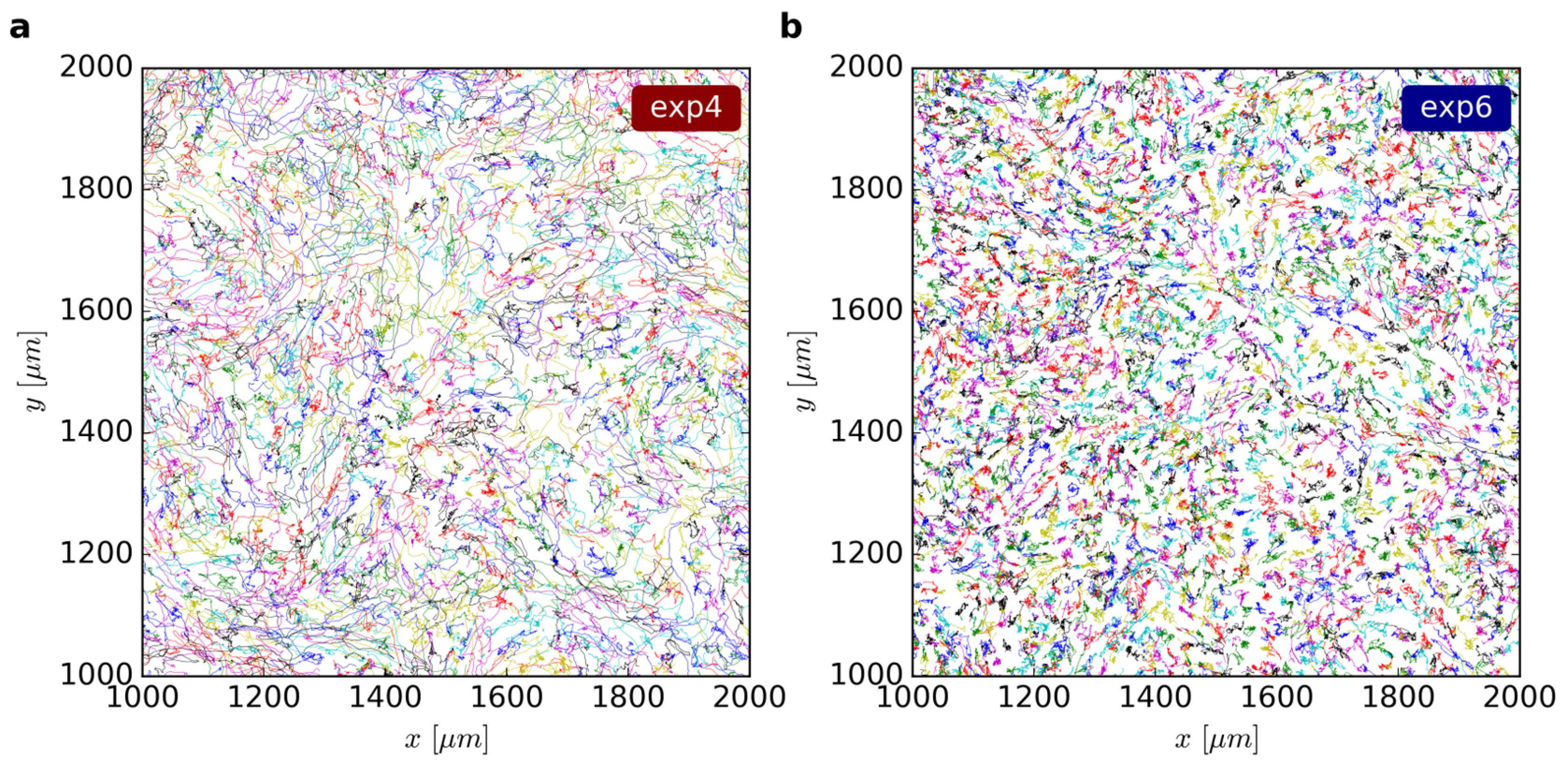
To analyze the micrographs with up to 50.000 cell signals per frame, we developed an automated image segmentation software. Using the programming language Python, we were able to extract the positions of the labeled cell nuclei, which were then connected for each cell to a trajectory as a function of time using the Crocker-Gier algorithm [9]. Final trajectories (Figure 1) of at least nine time steps were taken into account while the distance between consecutive positions must not exceed 10-12 µm, depending on the cell density. Cell velocities were calculated as the difference quotient of two consecutive cell positions.

The parameters and evidence of the models were estimated with the help of Bayesian data analysis (for details see [4]). A numerical analysis was performed with the MultiNest-sampling algorithm [10,11] in its Python implementation [12]. Uniform priors were applied for parameters N₀, β, t₀, A, A₁ and A₂. For all remaining parameters (α₀, α₁, σ, τ, τ₁, τ₂, A₀, c and two parameters adjusting the experimental error), Jeffreys’ priors were used. The agreement of data and model was assessed using a Gaussian likelihood function. The model means and scatterings were obtained by averaging over the resulting parameter samplings.

3. Results

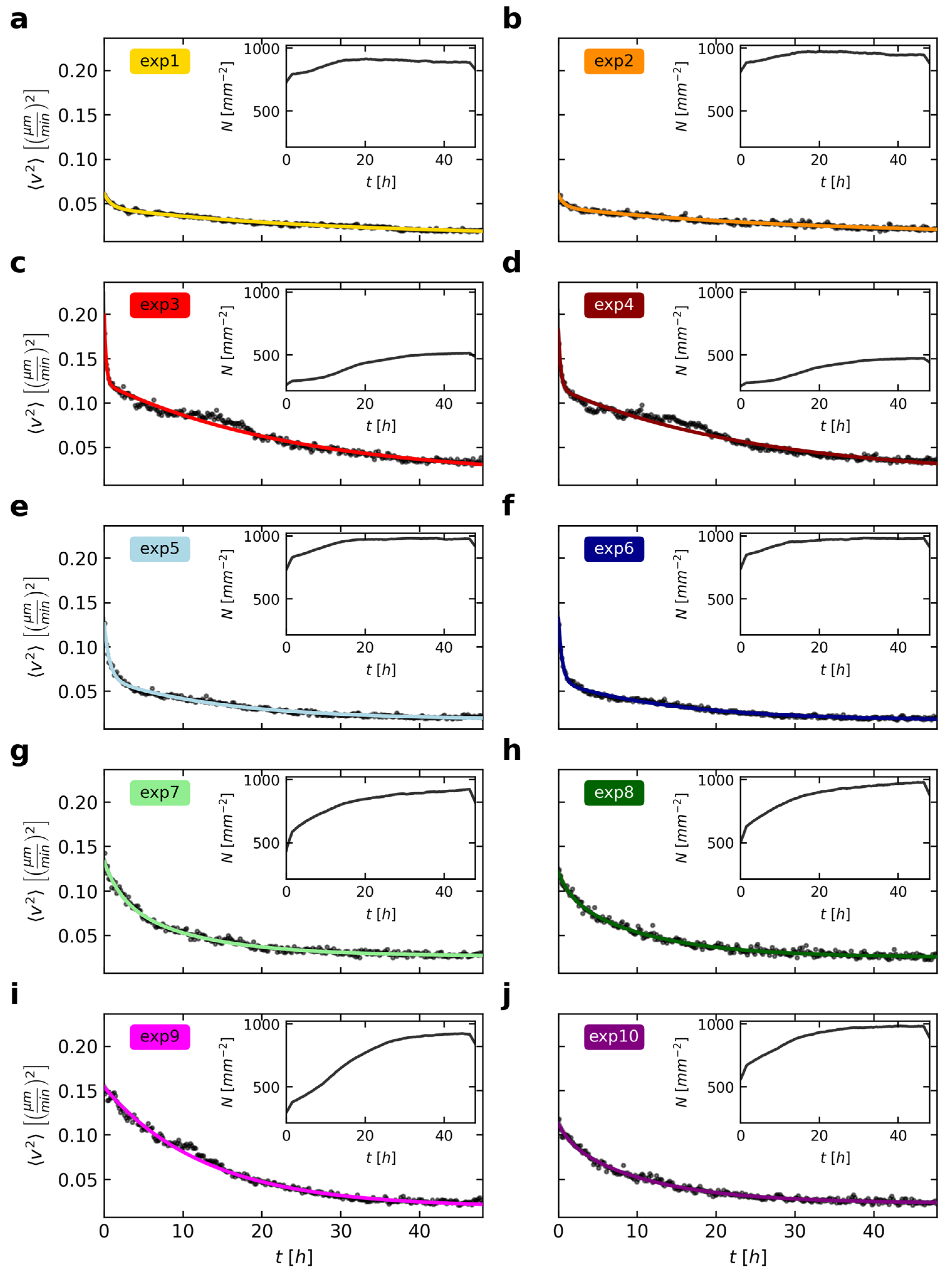
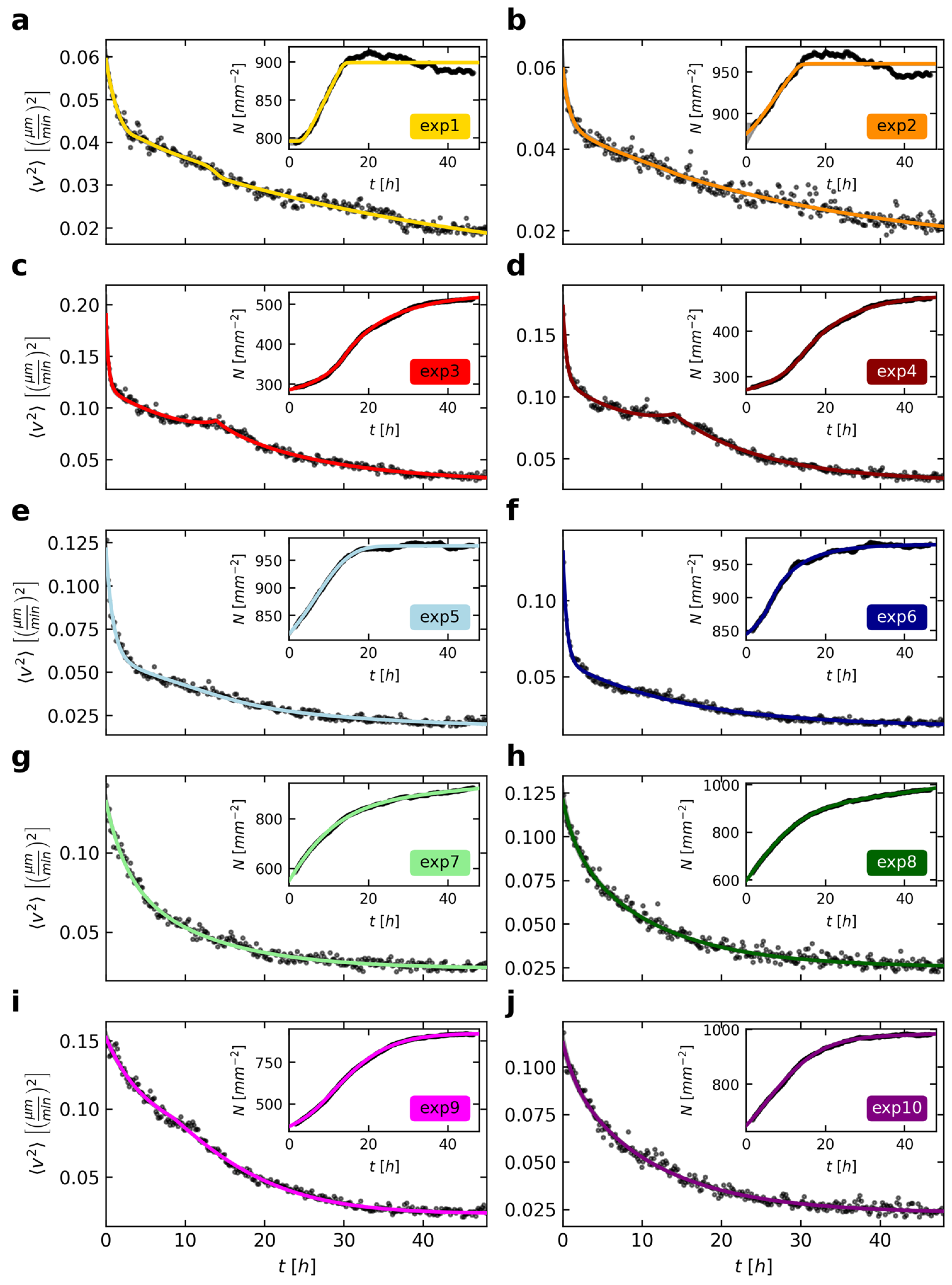
To obtain a first overview of the temporal development of cell movements, we calculated the mean squared velocity for each time step as the average of all cells that could be tracked for the entire observation time (Figure 2).

The cells decrease their mean squared velocity over time (Figure 2). However, this decline in velocities varies strongly between the ten experiments. We also noted different cell numbers at the beginning of the imaging as well as differing growth in the observed cell layers (Figure 2, insets). With the cells moving around and proliferating vividly, the cell arrangement usually gets more homogenous and macroscopically ordered over time. The resulting overall higher cell densities confine cell movements and therefore decrease mean squared velocities. To highlight this inverse relation, we chose the same axis limits for the velocities and densities for all experiments in Figure 2. If cell densities are high, then the corresponding velocities are, in comparison with the other experiments, quite low, and vice versa (e.g., Figure 2 a as opposed to c).

To develop a model describing the decline in mean cell velocities, the effect of several simultaneously ongoing biological processes should be quantified separately. First, we found that the cells rapidly slowed down at the start of the experiment. This is followed by a second, slower decline before the mean squared velocity seems to converge to a certain limit greater than zero for long times depending on the cell density. In some experiments (Figure 2c,d) the two declines seem to happen sequentially, whereas there are other examples (Figure 2h) that show a much smoother transition. We speculate that these two processes actually occur simultaneously with differing parameters since this seems to be more likely from a biological view. Hence, the little plateau, as observed especially in experiments 3 and 4 (Figure 2c,d) after 10 h, could be caused by a third phenomenon. Based on this consideration, we described the general decline using two exponential functions, with parameters A_1,2 and τ_1,2 and a basal squared velocity A₀.

$$〈v^2\left(t\right)〉=A_0+A_1{e}^{-\frac{t}{{\tau }_1}}+A_2{e}^{-\frac{t}{{\tau }_2}}.$$

(1)

As shown in Figure 2, this fit, obtained using Bayesian analysis, well captures the effects of the two processes that are slowing down the cells with the time scales of τ₁ and τ₂, ranging between ~16 and ~142 min and between ~655 and ~1780 min, respectively. These declines could be caused by the continuous cell aging and strengthening of cell-cell contacts. However, there are still data points that deviate from the model of Equation (1) during time ranges mainly within the first 20 h. Up to now, we did not include cell division activities in our model, which should be related to the velocities of cells: On the one hand, cells can move around more freely in areas with low density. They are less prone to collide with each other or have more space to change their directions. On the other hand, temporal phases of very active cell proliferation seem to be marked by a transiently constant or only very slowly decreasing cell velocity (see e.g., Figure 2c,d,i). Although this effect is short-lived, it shows that the separation of dividing cells can lead to accelerations in the system. By contrast, these cell divisions can also cause an overall deceleration due to an increasing confinement in densely packed cell clusters. That is why the mean squared velocities in experiments 3 and 4 show a transient plateau (Figure 2c,d) in their decline or why τ₂, as a means to describe the second, slower decline, might differ in these experiments.

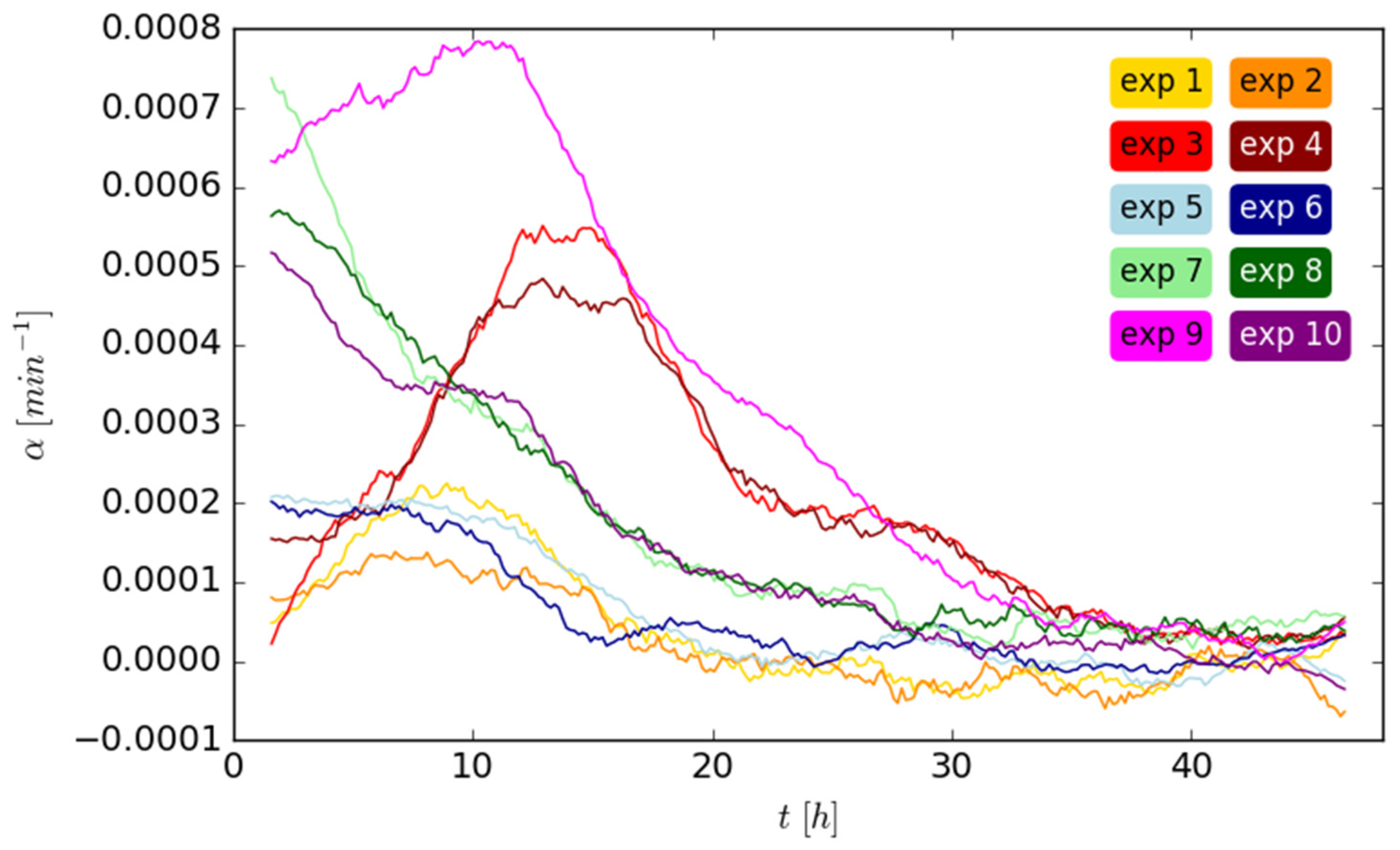
In order to quantify the connection between mean cell velocity and cell density, we calculated the relative changes in cell numbers for each time step (Figure 3).

The cells usually go through one phase of more intense cell division, which builds up at first and reaches a maximum before it subsides again. However, the onset, duration and strength of this phase differ strongly between the experiments. Occasionally, the maximum of cell division lies probably even before the start of the experimental observation. We can describe the relative increase α(t) in the cell numbers N per time t with

$$\alpha \left(t\right)=\frac{1}{N}\frac{dN}{dt}={\alpha }_0+{\alpha }_1{e}^{-{\left|\frac{t-t_0}{\sigma }\right|}^{\beta }}.$$

(2)

Here, α₀ describes the basal cell division, α₁ the strength, σ the duration and t₀ the time point of the maximum of the cell division phase. The exponent β changes the shape of the curve with β = 2 being the special case of a Gaussian function.

Since changes in cell density can modify the velocities of cells, we couple the cell division activity of Equation (2) linearly with factor c to the mean squared velocity of Equation (1). This temporarily raises the mean squared velocity during strong increases in cell numbers for c > 0.

$$〈v^2\left(t\right)〉=A_0+A_1{e}^{-\frac{t}{{\tau }_1}}+A_2{e}^{-\frac{t}{{\tau }_2}}+c\left({\alpha }_0+{\alpha }_1{e}^{-{\left|\frac{t-t_0}{\sigma }\right|}^{\beta }}\right).$$

(3)

Depending on the time point of the maximum cell division rate, the cell density can be calculated by integrating Equation (2), leading to the following result:

$$N\left(t\right)=\left\{\begin{array}{cc}{N}_0{e}^{\frac{{\alpha }_1\sigma }{\beta }\left\{\gamma \left(\frac{1}{\beta } , { \left(\frac{t-t_0}{\sigma }\right)}^{\beta }\right)-\gamma \left(\frac{1}{\beta } ,{ \left(-\frac{t_0}{\sigma }\right)}^{\beta }\right)\right\}+{\alpha }_{0}t}& if t_0<0 ,\\ N_0{e}^{-\frac{{\alpha }_1\sigma }{\beta }\left\{\gamma \left(\frac{1}{\beta } , { \left(\frac{t_0-t}{\sigma }\right)}^{\beta }\right)-\gamma \left(\frac{1}{\beta } ,{ \left(\frac{t_0}{\sigma }\right)}^{\beta }\right)\right\}+{\alpha }_{0}t}& if t_0>0 and t<t_{0 },\\ N_0{e}^{\frac{{\alpha }_1\sigma }{\beta }\left\{\gamma \left(\frac{1}{\beta } , { \left(\frac{t_0}{\sigma }\right)}^{\beta }\right)+\gamma \left(\frac{1}{\beta } ,{ \left(\frac{t-t_0}{\sigma }\right)}^{\beta }\right)\right\}+{\alpha }_{0}t}& if t_0>0 and t>t_0 .\end{array}\right.$$

(4)

Here, the lower incomplete gamma function is used according to Equation (5)

$$\gamma \left(a,x\right)=\underset{0}{\overset{x}{\int }}{t}^{a-1}{e}^{-t} dt$$

(5)

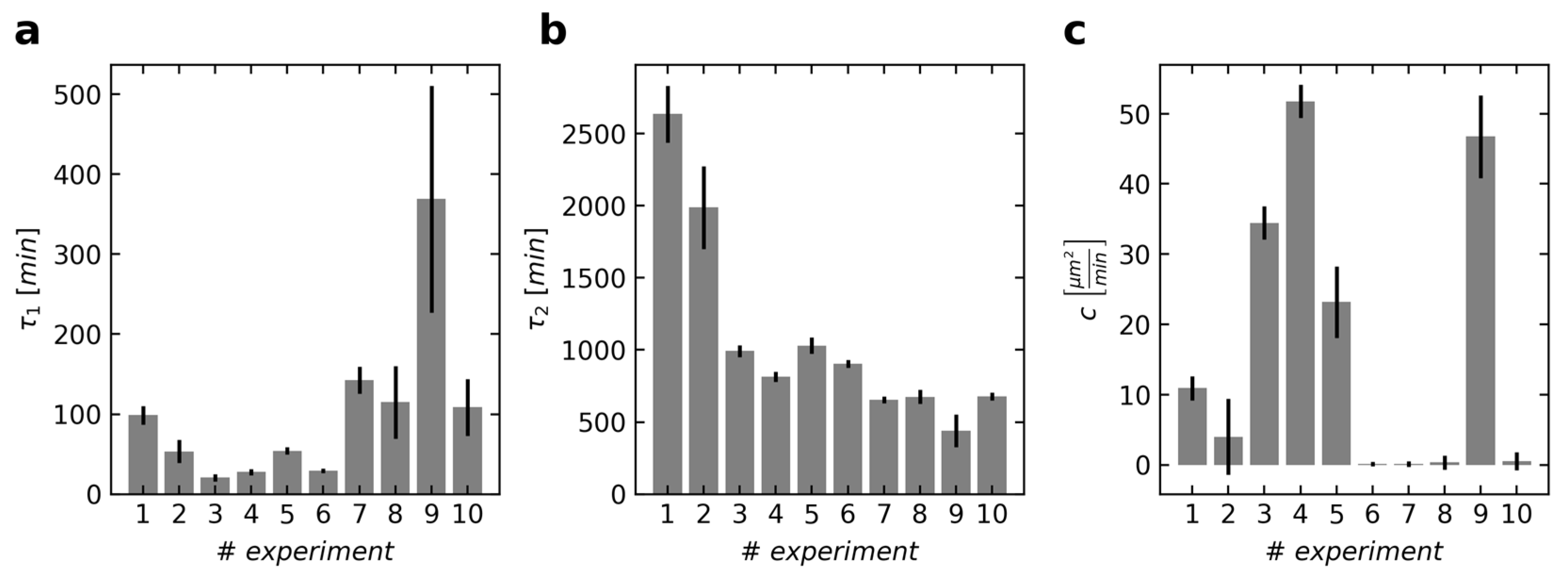
and N₀ denotes the initial cell number at t = 0. The obtained parameters of the simultaneous fit, calculated individually for each experiment, indicate that the trend of the velocities consists of a faster and a slower decline (Figure 4). After about one to three hours (elapsed time equals two τ₁), the cells have slowed down considerably (Figure 4a). After that time, the mean squared velocity decreases only slowly, with τ₂ usually being greater than 10 h (Figure 4b). The exception from these findings is the ninth experiment, where the two declines are merged and therefore difficult to separate. The first two experiments show a particularly slow decline since the cell density had always been high and the cells from this umbilical cord showed less activity. At large, the obtained values for the parameters are roughly of the same magnitude compared to the counterparts of the isolated fit (Equation (1) and Figure 2). This indicates that there are at least two time-dependent phases, with the cell division causing the time-independent alterations of the overall dynamics. This third influence is especially strong in experiments 3, 4 and 9, as indicated by parameter c (Figure 4c), where the mean squared velocities were also the highest. The first experiment shows slightly more cell division than the second while the mean squared velocities are almost the same (Figure 2a,b). Interestingly, the optimal parameters for the combined fit include a higher c and subsequently higher τ₁ and τ₂ (Figure 4) instead of these three parameters just being smaller. This might emphasize the importance of considering cell division in the model.

Based on the estimated parameters, we plotted the fits for the mean squared velocity and density (Figure 5).

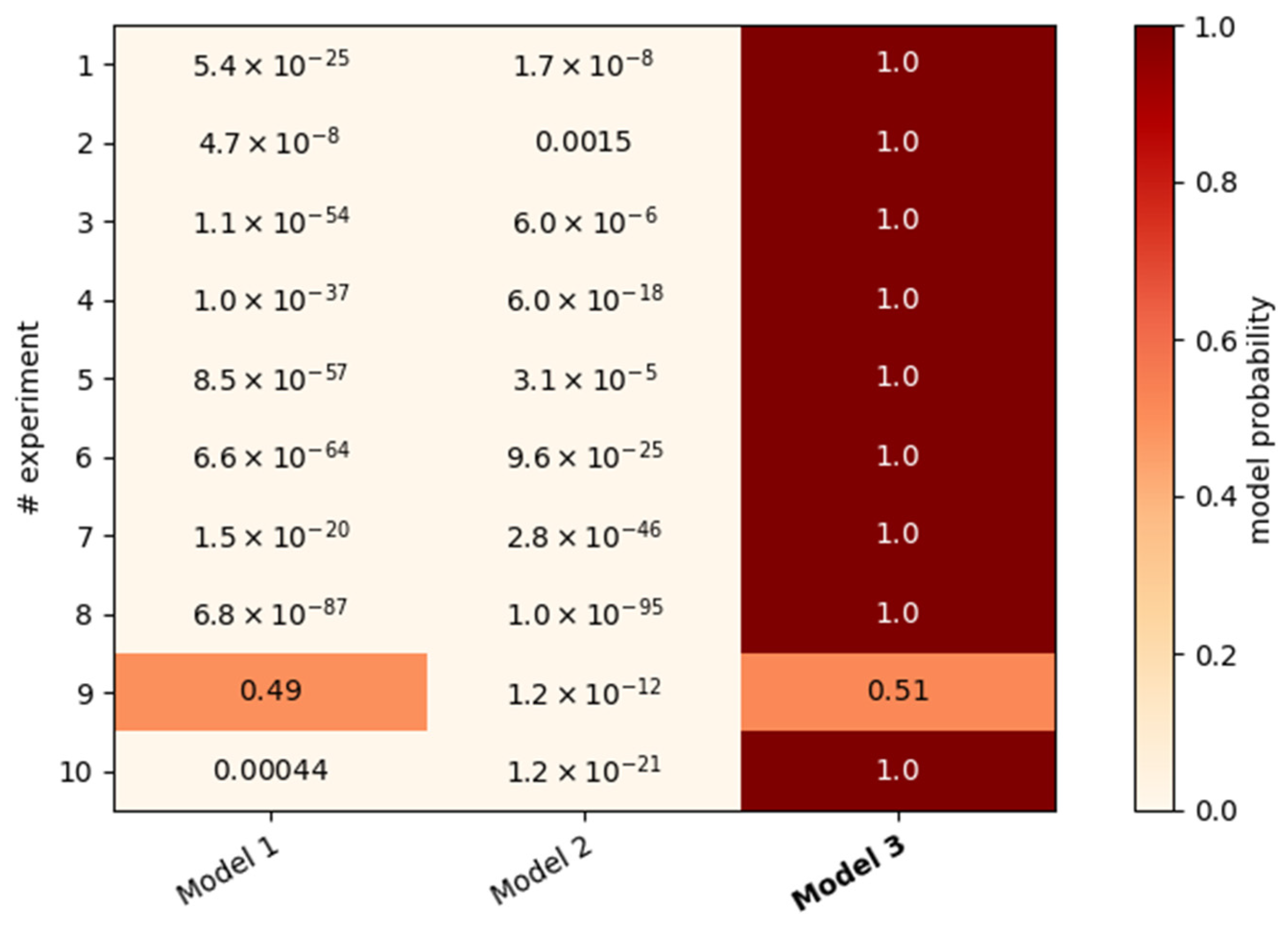
A comparison by eye shows that the model is suitable to describe the data of the cell densities as long as the cell numbers do not decrease (Figure 5a,b). Furthermore, the fit of the mean squared velocities was improved by the coupling to cell division activities, especially in experiments 3, 4 and 9. To verify that indeed two time scales are necessary to describe the overall decline, we compared the resulting Bayesian evidences with two alternative models. Model 1 (12 parameters) uses one exponential, Model 2 (13 parameters) uses one stretched exponential function in addition to the cell division term (

Table 1. Three different models (including one exponential, one stretched exponential or two exponential functions) were used for the fit of the mean squared velocity.

Model	Formula
1	$〈v^2\left(t\right)〉=A_0+A{e}^{-\frac{t}{\tau }}+c\left({\alpha }_0+{\alpha }_1{e}^{-{\left|\frac{t-t_0}{\sigma }\right|}^{\beta }}\right)$	(6)
2	$〈v^2\left(t\right)〉=A_0+A{e}^{-{\left|\frac{t}{\tau }\right|}^l}+c\left({\alpha }_0+{\alpha }_1{e}^{-{\left|\frac{t-t_0}{\sigma }\right|}^{\beta }}\right)$	(7)
3	$〈v^2\left(t\right)〉=A_0+A_1{e}^{-\frac{t}{{\tau }_1}}+A_2{e}^{-\frac{t}{{\tau }_2}}+c\left({\alpha }_0+{\alpha }_1{e}^{-{\left|\frac{t-t_0}{\sigma }\right|}^{\beta }}\right)$	(8)

). So far, Model 3 (14 parameters) was applied (Figure 5), which uses, in comparison with Model 1, an additional exponential function (2 in total).

The comparison of the evidences of the applied models shows a clear preference for Model 3 for nine out of ten experiments (Figure 6). This endorses the theory that there is usually a decline consisting of two parts with different temporal dynamics. Only the ninth experiment could also be described with just one exponential function. These cells showed the strongest and longest-lasting cell division phase out of all experiments, which led to a more than two-fold increase in cell density. This influence was incorporated into the fit for the velocity via a high coupling parameter c (Figure 4c). Thus, the effect of the proliferation-independent cell movements is less recognizable, especially because the processes occur largely simultaneously. This might have also caused the small difference between τ₁ and τ₂ and its higher error (Figure 4a,b).

4. Discussion

As long as the cells are motile and their numbers are not decreasing, Model 3 is able to fit the cell density and mean squared velocity for all experiments despite their interindividual differences. Bayesian analysis was used to quantify the parameters of the suspected underlying biological processes. It is noteworthy that the parameter estimation succeeded in finding suitable results for the parameters included in both fits, promoting the idea that not only the cell density but also the velocities are positively influenced by cell divisions. It should be noted that the number of cell divisions was derived from the changes in cell density. The actual number of cell divisions could be higher, since we did not quantify the number of cell deaths. The comparison of three different models showed that the best approach consists of the sum of two exponentially decaying functions. We considered in all models the relatively small but accumulating amount of increased velocities generated by cell division. Although the two new cells shift initially only a few micrometers apart from each other in opposite directions, the influences of several cell divisions do not even each other out. Nevertheless, it is taken into account that strong cell proliferation increases cell density and eventually diminishes cell velocities. The basic velocity level could be connected to the absolute value of the cell numbers. Furthermore, the effect of aging or increasing cell localization on the dynamics might be fitted in a better way than with just an exponential function. Here, the necessity to use two of these functions for the velocity already shows that there are many more biophysical mechanisms influencing cell movements. In the future, we will use and extend this approach to assess other aspects of cell migration.

References

1. Michaelis, U.R. Mechanisms of endothelial cell migration. Cell. Mol. Life Sci. 2014, 71, 4131–4148. [Google Scholar] [CrossRef] [PubMed]
2. Friedl, P.; Gilmour, D. Collective cell migration in morphogenesis, regeneration and cancer. Nat. Rev. Mol. Cell Biol. 2009, 10, 445–457. [Google Scholar] [CrossRef] [PubMed]
3. Lämmermann, T.; Germain, R.N. The multiple faces of leukocyte interstitial migration. Semin. Immunopathol. 2014, 36, 227–251. [Google Scholar] [CrossRef] [PubMed]
4. Dieterich, P.; Lindemann, O.; Moskopp, M.L.; Tauzin, S.; Huttenlocher, A.; Klages, R.; Chechkin, A.; Schwab, A. Anomalous diffusion and asymmetric tempering memory in neutrophil chemotaxis. PLoS Comput. Biol. 2022, 18, e1010089. [Google Scholar] [CrossRef] [PubMed]
5. Lo, C.M.; Wang, H.B.; Dembo, M.; Wang, Y.L. Cell movement is guided by the rigidity of the substrate. Biophys. J. 2000, 79, 144–152. [Google Scholar] [CrossRef] [PubMed]
6. Peyton, S.R.; Putnam, A.J. Extracellular matrix rigidity governs smooth muscle cell motility in a biphasic fashion. J. Cell Physiol. 2005, 204, 198–209. [Google Scholar] [CrossRef] [PubMed]
7. Rørth, P. Collective cell migration. Annu. Rev. Cell Dev. Biol. 2009, 25, 407–429. [Google Scholar] [CrossRef] [PubMed]
8. Khedr, S.; Deussen, A.; Kopaliani, I.; Zatschler, B.; Martin, M. Effects of tryptophan-containing peptides on angiotensin-converting enzyme activity and vessel tone ex vivo and in vivo. Eur. J. Nutr. 2018, 57, 907–915. [Google Scholar] [CrossRef] [PubMed]
9. Crocker, J.; Grier, D. Methods of Digital Video Microscopy for Colloidal Studies. J. Colloid Interface Sci. 1996, 179, 298–310. [Google Scholar] [CrossRef]
10. Skilling, J. Nested sampling for general Bayesian computation. Bayesian Anal. 2006, 1, 833–859. [Google Scholar] [CrossRef]
11. Feroz, F.; Hobson, M.P.; Bridges, M. MultiNest: An efficient and robust Bayesian inference tool for cosmology and particle physics. Mon. Not. R. Astron. Soc. 2009, 398, 1601–1614. [Google Scholar] [CrossRef]
12. Buchner, J.; Georgakakis, A.; Nandra, K.; Hsu, L.; Rangel, C.; Brightman, M.; Merloni, A.; Salvato, M.; Donley, J.L.; Kocevski, D. X-ray spectral modelling of the AGN obscuring region in the CDFS: Bayesian model selection and catalogue. Astron. Astrophys. 2014, 564, A125. [Google Scholar] [CrossRef]
Figure 1. In a section (1 mm2) of the cell layer, all cell trajectories are shown for the experiments 4 (a) and 6 (b). The trajectories are labeled sequentially with one out of seven colors in the order of their first appearance and the attributed cell number. The overall cell density in (a) is much lower than in (b). This leads to different dynamics and pattern formation.
Psf 09 00011 g001
Figure 2. The mean squared velocities and cell densities (inset) are shown for each time step in all ten experiments (black dots, aj). Additionally, the mean squared velocities are fitted with two exponential functions (Equation (1), solid colored line). In certain time intervals of the experiments (especially in c,d,i), the fit transiently deviates from the course of the data points. The quite small uncertainties (two standard deviations) of the model fit are marked as a gray area (barely visible). The calculation of the velocities is based on all cells that could be tracked for the entire duration of the experiment (48 h). The values for the cell densities consider all cells with the exception of the boundary area. The cell numbers in the first and last nine time steps are artificially lower due to the defined minimum trajectory length during cell tracking. Experiments with cells from the same umbilical cord are shown in the same row.
Psf 09 00011 g002
Figure 3. The changes in cell numbers α(t) (Equation (2)) are calculated for each time step. A uniform filter with a size of 300 min was applied to smoothen the data. Due to the defined minimum length of cell trajectories during image analysis, the first and last nine time steps were discarded.
Psf 09 00011 g003
Figure 4. The mean and standard deviation for the estimated parameters τ1 (a), τ2 (b) and c (c) are shown for each experiment. Here, τ1 and τ2 describe the two time scales with which the exponential functions are decreasing. Parameter c depicts the coupling strength between the rate of cell division and the mean squared velocity.
Psf 09 00011 g004
Figure 5. The fits to the mean squared velocity (aj), as shown in Figure 2, were improved using Equation (3). The shown data of the cell density (inset) was fitted simultaneously for each experiment according to Equation (4). The quite small uncertainties (two standard deviations) of the model fit are represented as a gray area (almost only visible in the inset of (b)). Note that the ranges of the y-axes are optimally adjusted to each data set in contrast to Figure 2.
Psf 09 00011 g005
Figure 6. Three models (Table 1) were used for the simultaneous fit of the mean squared velocity and density. The evidence, obtained by Bayesian analysis, is used to compare the accuracy of the different models. The model probability is shown color-coded and in numbers for each experiment.
Psf 09 00011 g006