
Proximal Nested Sampling with Data-Driven Priors for Physical Scientists †


Abstract
:1. Introduction
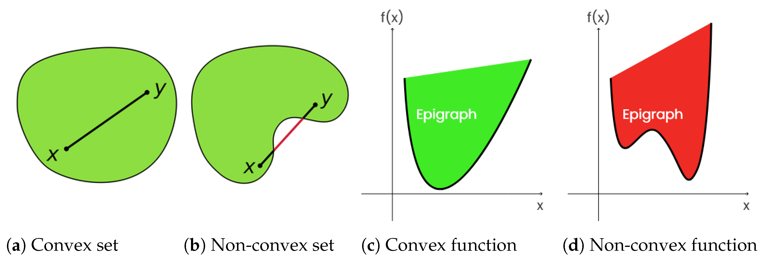
2. Convexity and Proximal Calculus
2.1. Convexity
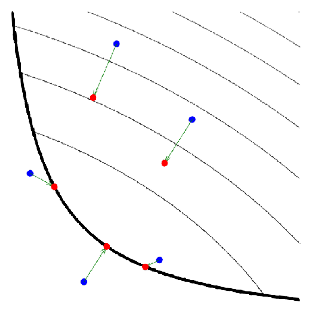
2.2. Proximity Operator
2.3. Moreau–Yosida Regularisation
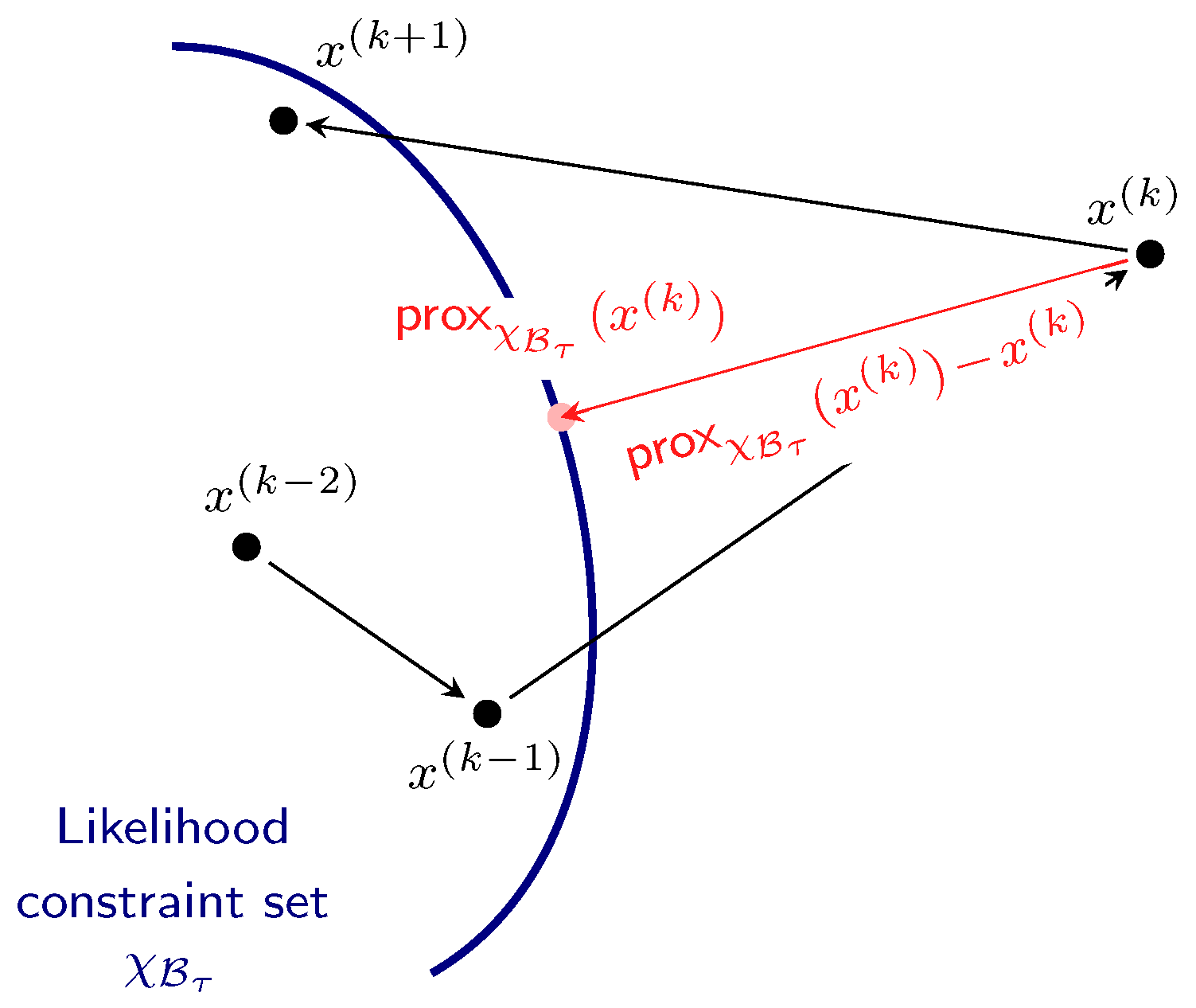
3. Proximal Nested Sampling
3.1. Constrained Sampling Formulation
3.2. Langevin MCMC Sampling
3.3. Proximal Nested Sampling Framework
3.4. Explicit Forms of Proximal Nested Sampling
- ;
- .
4. Deep Data-Driven Priors
4.1. Tweedie’s Formula and Data-Driven Priors
4.2. Proximal Nested Sampling with Data-Driven Priors
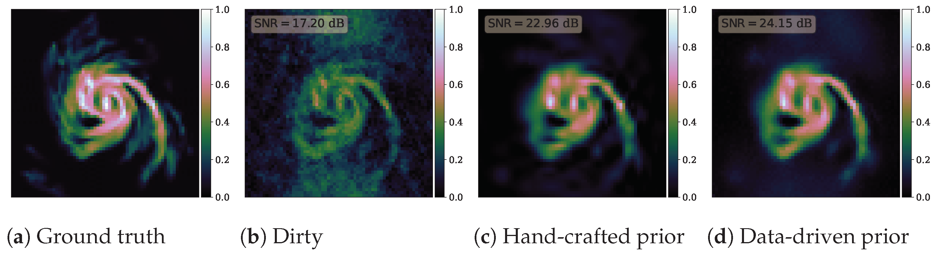
5. Numerical Experiments
6. Conclusions
Author Contributions
Funding
Institutional Review Board Statement
Informed Consent Statement
Data Availability Statement
Conflicts of Interest
References
- Robert, C.P. The Bayesian Choice; Springer: New York, NY, USA, 2007. [Google Scholar]
- Ashton, G.; Bernstein, N.; Buchner, J.; Chen, X.; Csányi, G.; Fowlie, A.; Feroz, F.; Griffiths, M.; Handley, W.; Habeck, M.; et al. Nested sampling for physical scientists. Nat. Rev. Methods Prim. 2022, 2, 39. [Google Scholar] [CrossRef]
- Skilling, J. Nested sampling for general Bayesian computation. Bayesian Anal. 2006, 1, 833–859. [Google Scholar] [CrossRef]
- Mukherjee, P.; Parkinson, D.; Liddle, A.R. A nested sampling algorithm for cosmological model selection. Astrophys. J. 2006, 638, L51–L54. [Google Scholar] [CrossRef]
- Feroz, F.; Hobson, M.P. Multimodal nested sampling: An efficient and robust alternative to MCMC methods for astronomical data analysis. Mon. Not. R. Astron. Soc. (MNRAS) 2008, 384, 449–463. [Google Scholar] [CrossRef]
- Feroz, F.; Hobson, M.P.; Bridges, M. MULTINEST: An efficient and robust Bayesian inference tool for cosmology and particle physics. Mon. Not. R. Astron. Soc. (MNRAS) 2009, 398, 1601–1614. [Google Scholar] [CrossRef]
- Handley, W.J.; Hobson, M.P.; Lasenby, A.N. POLYCHORD: Nested sampling for cosmology. Mon. Not. R. Astron. Soc. Lett. 2015, 450, L61–L65. [Google Scholar] [CrossRef]
- Buchner, J. Nested sampling methods. arXiv 2021, arXiv:2101.09675. [Google Scholar] [CrossRef]
- McEwen, J.D.; Wallis, C.G.R.; Price, M.A.; Docherty, M.M. Machine learning assisted Bayesian model comparison: The learnt harmonic mean estimator. arXiv 2022, arXiv:2111.12720. [Google Scholar]
- Spurio Mancini, A.; Docherty, M.M.; Price, M.A.; McEwen, J.D. Bayesian model comparison for simulation-based inference. RAS Tech. Instrum. 2023, 2, 710–722. [Google Scholar] [CrossRef]
- Polanska, A.; Price, M.A.; Spurio Mancini, A.; McEwen, J.D. Learned harmonic mean estimation of the marginal likelihood with normalising flows. Phys. Sci. Forum 2023, 9, 10. [Google Scholar] [CrossRef]
- Cai, X.; McEwen, J.D.; Pereyra, M. Proximal nested sampling for high-dimensional Bayesian model selection. Stat. Comput. 2022, 32, 87. [Google Scholar] [CrossRef]
- Combettes, P.; Pesquet, J.C. Proximal Splitting Methods in Signal Processing; Springer: New York, NY, USA, 2011; pp. 185–212. [Google Scholar]
- Parikh, N.; Boyd, S. Proximal algorithms. Found. Trends Optim. 2013, 1, 123–231. [Google Scholar]
- Pereyra, M. Proximal Markov chain Monte Carlo algorithms. Stat. Comput. 2016, 26, 745–760. [Google Scholar] [CrossRef]
- Durmus, A.; Moulines, E.; Pereyra, M. Efficient Bayesian computation by proximal Markov chain Monte Carlo: When Langevin meets Moreau. SIAM J. Imaging Sci. 2018, 1, 473–506. [Google Scholar] [CrossRef]
- Skilling, J. Bayesian computation in big spaces-nested sampling and Galilean Monte Carlo. In Proceedings of the AIP Conference 31st American Institute of Physics, Zurich, Switzerland, 29 July–3 August 2012; Volume 1443, pp. 145–156. [Google Scholar]
- Betancourt, M. Nested sampling with constrained hamiltonian monte carlo. AIP Conf. Proc. 2011, 1305, 165–172. [Google Scholar] [CrossRef]
- Laumont, R.; Bortoli, V.D.; Almansa, A.; Delon, J.; Durmus, A.; Pereyra, M. Bayesian imaging using Plug & Play priors: When Langevin meets Tweedie. SIAM J. Imaging Sci. 2022, 15, 701–737. [Google Scholar]
- Robbins, H. An Empirical Bayes Approach to Statistics. In Proceedings of the Third Berkeley Symposium on Mathematical Statistics and Probability, Berkeley, CA, USA, December 1954 and July–August 1955; University of California Press: Berkeley, CA, USA, 1956; Volume 3.1, pp. 157–163. [Google Scholar]
- Efron, B. Tweedie’s formula and selection bias. J. Am. Stat. Assoc. 2011, 106, 1602–1614. [Google Scholar] [CrossRef] [PubMed]
- Kim, K.; Ye, J.C. Noise2score: Tweedie’s approach to self-supervised image denoising without clean images. Adv. Neural Inf. Process. Syst. 2021, 34, 864–874. [Google Scholar]
- Chung, H.; Sim, B.; Ryu, D.; Ye, J.C. Improving diffusion models for inverse problems using manifold constraints. arXiv 2022, arXiv:2206.00941. [Google Scholar]
- Sohl-Dickstein, J.; Weiss, E.; Maheswaranathan, N.; Ganguli, S. Deep unsupervised learning using nonequilibrium thermodynamics. PMLR 2015, 37, 2256–2265. [Google Scholar]
- Song, Y.; Ermon, S. Generative modeling by estimating gradients of the data distribution. In Proceedings of the 33rd Annual Conference on Neural Information Processing Systems (NeurIPS 2019), Vancouver, Canada, 8–14 December 2019. [Google Scholar]
- Song, Y.; Ermon, S. Improved techniques for training score-based generative models. Adv. Neural Inf. Process. Syst. 2020, 33, 12438–12448. [Google Scholar]
- Song, Y.; Sohl-Dickstein, J.; Kingma, D.P.; Kumar, A.; Ermon, S.; Poole, B. Score-based generative modeling through stochastic differential equations. arXiv 2020, arXiv:2011.13456. [Google Scholar]
- Rombach, R.; Blattmann, A.; Lorenz, D.; Esser, P.; Ommer, B. High-resolution image synthesis with latent diffusion models. In Proceedings of the IEEE/CVF Conference on Computer Vision and Pattern Recognition, New Orleans, LA, USA, 18–24 June 2022; pp. 10684–10695. [Google Scholar]
- Venkatakrishnan, S.V.; Bouman, C.A.; Wohlberg, B. Plug-and-play priors for model based reconstruction. In Proceedings of the 2013 IEEE Global Conference on Signal and Information Processing, IEEE, Austin, TX, USA, 3–5 December 2013; pp. 945–948. [Google Scholar]
- Ryu, E.; Liu, J.; Wang, S.; Chen, X.; Wang, Z.; Yin, W. Plug-and-play methods provably converge with properly trained denoisers. In Proceedings of the International Conference on Machine Learning. PMLR, Long Beach, CA, USA, 9–15 June 2019; pp. 5546–5557. [Google Scholar]
- Nelson, D.; Springel, V.; Pillepich, A.; Rodriguez-Gomez, V.; Torrey, P.; Genel, S.; Vogelsberger, M.; Pakmor, R.; Marinacci, F.; Weinberger, R.; et al. The IllustrisTNG Simulations: Public Data Release. Comput. Astrophys. Cosmol. 2019, 6, 2. [Google Scholar] [CrossRef]


Disclaimer/Publisher’s Note: The statements, opinions and data contained in all publications are solely those of the individual author(s) and contributor(s) and not of MDPI and/or the editor(s). MDPI and/or the editor(s) disclaim responsibility for any injury to people or property resulting from any ideas, methods, instructions or products referred to in the content. |
© 2023 by the authors. Licensee MDPI, Basel, Switzerland. This article is an open access article distributed under the terms and conditions of the Creative Commons Attribution (CC BY) license (https://creativecommons.org/licenses/by/4.0/).
Share and Cite
McEwen, J.D.; Liaudat, T.I.; Price, M.A.; Cai, X.; Pereyra, M. Proximal Nested Sampling with Data-Driven Priors for Physical Scientists. Phys. Sci. Forum 2023, 9, 13. https://doi.org/10.3390/psf2023009013
McEwen JD, Liaudat TI, Price MA, Cai X, Pereyra M. Proximal Nested Sampling with Data-Driven Priors for Physical Scientists. Physical Sciences Forum. 2023; 9(1):13. https://doi.org/10.3390/psf2023009013
Chicago/Turabian StyleMcEwen, Jason D., Tobías I. Liaudat, Matthew A. Price, Xiaohao Cai, and Marcelo Pereyra. 2023. "Proximal Nested Sampling with Data-Driven Priors for Physical Scientists" Physical Sciences Forum 9, no. 1: 13. https://doi.org/10.3390/psf2023009013