Variational Bayesian Approximation (VBA) with Exponential Families and Covariance Estimation ^†

Abstract

Variational Bayesian Approximation (VBA) is a fast technique for approximating Bayesian computation. The main idea is to assess the joint posterior distribution of all the unknown variables with a simple expression. Mean–Field Variational Bayesian Approximation (MFVBA) is a particular case developed for large–scale problems where the approximated probability law is separable in all variables. A well–known drawback of MFVBA is that it tends to underestimate the variances in the variables, even though it estimates the means well. It can lead to poor inference results. We can obtain a fixed point algorithm to evaluate the means in exponential families for the approximating distribution. However, this does not solve the problem of underestimating the variances. In this paper, we propose a modified method of VBA with exponential families to first estimate the posterior mean and then improve the estimation of the posterior covariance. We demonstrate the performance of the procedure with an example.

1. Introduction

Bayesian computation uses Bayes’ theorem to revise the probabilities of unknowns based on prior knowledge and data. When the likelihood expressions and prior are available, we can get the expression of the posterior law. However, this expression needs the denominator integral computation of the Bayes formula, called evidence. Approximate Bayesian Computation (ABC) are a class of algorithms used to perform Bayesian computation without exactly computing the evidence. The first class of these methods generate samples from the posterior law. We can mention all of the Monte Carlo sampling methods, such as slice sampling, nested sampling, and Markov chain Monte Carlo (MCMC) methods. The second category of these methods includes those that directly compute the means and variances, such as the Variational Bayesian Approximation (VBA) methods.

MCMC is a class of algorithms for sampling from a probability distribution and estimating the posterior distribution. Metropolis et al. (1953) [1] introduced the first MCMC algorithm called the Metropolis algorithm. Hastings (1970) [2] brought it closer to applied statistics, generalizing the Metropolis algorithm for asymmetric proposal distributions.

VBA methods were introduced by Jordan et al. (1998) [3]. They were motivated by the demand to improve the Bayesian inference for large and complex models intractable by conventional methods such as MCMC. VBA is a fast and robust scheme to perform Bayesian computations in high–dimensional problems. The main idea is to approximate the high–complexity posterior probability law with a simple and lower–complexity probability law using the Kullback–Leibler divergence as the approximation criterion.

In many cases, the VBA methods are faster than the MCMC methods. VBA can release two types of posterior approximations. The first is the free–form product of distributions such as the conjugated exponential family known as the Mean–Field Approximation (MFA). The second one is the fixed–form for posterior distributions like multivariate Gaussian with a proper parametrization for the model, Sarkka and Nummenmaa (2009) [4]. MFA is a general approach in the graphical models, particularly for the hierarchical Bayesian models.

The foundation of VBA is minimizing the Kullback–Leibler divergence (KL) between the approximated probability distribution and the exact posterior distribution. Rohde and Wand (2016) [5] worked on semi–parametric Mean–Field Variational Bayesian Approximation (MFVBA) as a combination of the KL measure and MFA. A significant drawback of MFVBA is that it underestimates the variable uncertainties and is uninformed concerning the variable covariance of models. Giordano et al. (2015, 2018) [6,7] rectified the MFVBA and named Linear Response Variational Bayes (LRVB) as being able to provide proper uncertainties.

MFVBA is a valuable approximation method for estimating the posterior mean in the Bayesian framework. While using an exponential family for approximation, we get a fixed point algorithm for reckoning the means. In this paper, we show how to use VBA with exponential families to approximate the posterior means and simultaneously evaluate the posterior covariance more precisely. Via an example, we also compare the MFVBA and MCMC posterior distributions.

This paper’s organization is as follows: In Section 2, we demonstrate the main idea of MFVBA with a particular case in exponential family (EF) distributions. In Section 3, we modify the covariance matrix resulting from the MFVBA to get a better approximation. In Section 4, we give details of the covariance matrix expression in EF. We show that the covariance computation needs high–dimensional matrix inversion, which is very costly in high–dimensional problems. In Section 5, we provide an example of how to compute the posterior distribution and compare the computational costs of the proposed method and the MCMC. In Section 6, we present the main conclusion on the paper content.

2. Mean–Field Variational Bayesian Approximation (MFVBA)

VBA approximates posterior distributions when the exact expression of the posterior is too complex or costly. MFA simplifies the VBA by assuming that the final distribution is factorized into independent margins, which means that each unknown parameter has its distribution independent of the others.

Suppose that p is approximated by $q^{*}$ and $\mathit{\theta }$ is the unknown vector of parameters. We define $\mathit{V}={\mathrm{Cov}}_{q^{*}}\left(\mathit{\theta }\right)$ and $\mathbf{\Sigma }={\mathrm{Cov}}_p\left(\mathit{\theta }\right)$. We know that $\mathit{V}<\mathbf{\Sigma }$. $\mathit{V}$ is a poor estimate (underestimate) of $\mathbf{\Sigma }$ even if ${\mathit{m}}^{*}=E_{q^{*}}\left\{\mathit{\theta }\right\}=E_p\left\{\mathit{\theta }\right\}$. The question is how to find a better estimate for $\mathbf{\Sigma }$. One solution for $\mathbf{\Sigma }$ in the case of the exponential family, proposed by Giordano et al. $\left(2015\right)$ [6], is $\mathbf{\Sigma }={(\mathit{I}-\mathit{V}\mathit{H})}^{-1}\mathit{V}$ via the LRVB method, where $\mathit{I}$ and $\mathit{H}$ are an identity matrix and Hessian matrix of the log probability $lnp$, respectively. To show this, let us go through the details step by step.

2.1. Main Idea

• General Bayesian framework: Given the likelihood $p\left(\mathcal{D}\right|\mathit{\theta })$ and the prior $p\left(\mathit{\theta }\right)$, the expression of the posterior $p\left(\mathit{\theta }\right|\mathcal{D})$ is given by:

  $$p\left(\mathit{\theta }\right|\mathcal{D})=\frac{p\left(\mathcal{D}\right|\mathit{\theta }\left)p\right(\mathit{\theta })}{p\left(\mathcal{D}\right)}.$$

  (1)
• MFVBA: Approximate $p\left(\mathit{\theta }\right|x)$ by a separable $q\left(\mathit{\theta }\right)$:

  $$q\left(\mathit{\theta }\right)=\prod _j{q}_j\left({\theta }_j\right),$$

  (2)

  by minimizing:

  $$\mathrm{KL}\left[q:p\right]=\int qln\frac{q}{p}={\mathrm{E}}_q\left\{lnq\right\}-{\mathrm{E}}_q\left\{lnp\right\}.$$

  (3)
• Noting by $L={\mathrm{E}}_q\left\{lnp\right\}$ the expected posterior likelihood and by $S=-{\mathrm{E}}_q\left\{lnq\right\}$ the entropy of q, we can also write:

  $$q^{*}=arg\underset{q}{min}\left\{\mathrm{KL}\left[q:p\right]\right\}=arg\underset{q}{max}\left\{E=S+L\right\}.$$

  (4)
• E is the evidence lower bound.

2.2. VBA and Exponential Family

• If q is chosen to be in an exponential family:

  $$q\left(\mathit{\theta }\right|\mathit{\eta })=exp\left[{\mathit{\eta }}^{\prime }\mathit{\theta }-A\left(\mathit{\eta }\right)\right],$$

  (5)

  then it is entirely characterized by its mean $\mathit{m}={\mathrm{E}}_q\left\{\mathit{\theta }\right\}$ and so is:

  $$q^{*}\left(\mathit{\theta }\right|{\mathit{\eta }}^{*})=exp\left[{{\mathit{\eta }}^{*}}^{\prime }\mathit{\theta }-A\left({\mathit{\eta }}^{*}\right)\right],$$

  (6)

  then the same characterization by the mean ${\mathit{m}}^{*}={\mathrm{E}}_{q^{*}}\left\{\mathit{\theta }\right\}$.
• We can then define the objective E as a function of $\mathit{m}$, and the first–order condition of the optimality is:

  $$\frac{\partial E}{\partial \mathit{m}}{|}_{\mathit{m}=\mathit{m}*}=0.$$

  (7)

2.3. MFVBA, Exponential Family (EF) and Fixed Point Algorithm

• VBA+exponential family with ${\mathrm{E}}_q\left\{\mathit{\theta }\right\}$:

  $$\frac{\partial E}{\partial \mathit{m}}{|}_{\mathit{m}=\mathit{m}*}=0\to \frac{\partial E}{\partial \mathit{m}}{|}_{\mathit{m}=\mathit{m}*}+\mathit{m}=\mathit{m}\to M\left(\mathit{m}\right)=\mathit{m}.$$

  (8)
• Iterating on this fixed point algorithm:

  $$M\left(\mathit{m}\right)={\mathit{m}}^{(k-1)}\mathrm{with}\mathit{M}\left(\mathit{m}\right):=\frac{\partial E}{\partial \mathit{m}}+\mathit{m},$$

  (9)

  converges to $\mathit{m}*={\mathrm{E}}_{q^{*}}\left\{\mathit{\theta }\right\}$.

3. VBA, EF and Covariance Estimation

• Noting from $\mathit{V}={\mathrm{Cov}}_{q^{*}}\left(\mathit{\theta }\right)$ and $\mathbf{\Sigma }={\mathrm{Cov}}_p\left(\mathit{\theta }\right)$, we know that $\mathit{V}<\mathbf{\Sigma }$.
• $\mathit{V}$ is a poor estimate (underestimate) of $\mathbf{\Sigma }$ even if ${\mathit{m}}^{*}={\mathrm{E}}_{q^{*}}\left\{\mathit{\theta }\right\}={\mathrm{E}}_p\left\{\mathit{\theta }\right\}$.
• The question is now: How to find a better estimate for $\mathbf{\Sigma }$.
• One solution proposed by Giordano et al. $\left(2015\right)$ [6] is the LRVB.
  The main idea is to perturb $p\left(\mathit{\theta }\right|x)$ by some exponential family to obtain $p_{\mathit{t}}\left(\mathit{\theta }\right|x)$:

  $$p_{\mathit{t}}\left(\mathit{\theta }\right|x)=p\left(\mathit{\theta }\right|x)exp\left[{\mathit{t}}^{\prime }\mathit{\theta }+C\left(\mathit{t}\right)\right]$$

  (10)

  such that:

  $$ln{p}_{\mathit{t}}\left(\mathit{\theta }\right|x)=lnp\left(\mathit{\theta }\right|x)+{\mathit{t}}^{\prime }\mathit{\theta }+C\left(\mathit{t}\right)$$

  (11)
• $C\left(\mathit{t}\right)$ is the cumulate generating function of $p_{\mathit{t}}\left(\mathit{\theta }\right|x)$, so

  $$\mathbf{\Sigma }={\mathrm{Cov}}_p\left(\mathit{\theta }\right)=\frac{{\partial }^{2}C\left(\mathit{t}\right)}{\partial {\mathit{t}}^{\prime }\partial \mathit{t}}{|}_{\mathit{t}=\mathbf{0}}=\frac{\partial {\mathrm{E}}_{p_{\mathit{t}}}\left\{\mathit{\theta }\right\}}{\partial {\mathit{t}}^{\prime }}{|}_{\mathit{t}=\mathbf{0}}=\frac{\partial {\mathit{m}}_{\mathit{t}}^{*}}{\partial {\mathit{t}}^{\prime }}{|}_{\mathit{t}=\mathbf{0}}$$

  (12)

4. Linear Perturbation Method for Better Covariance Estimation

To summarize this method:

• Perturb $p\left(\mathit{\theta }\right|x)$ by an exponential family term to obtain:

  $$p_{\mathit{t}}\left(\mathit{\theta }\right|x)=p\left(\mathit{\theta }\right|x)exp\left[{\mathit{t}}^{\prime }\mathit{\theta }+C\left(\mathit{t}\right)\right].$$
  Thus, we have:

  $$\begin{array}{cc}\hfill -\mathrm{KL}\left[q:p_{\mathit{t}}\right]=& -\mathrm{KL}\left[q:p\right]+{\mathit{t}}^{\prime }\mathit{m}⟶E_{\mathit{t}}=E+{\mathit{t}}^{\prime }\mathit{m},\hfill \\ \hfill \frac{\partial E}{\partial \mathit{m}}=& 0⟶\mathit{m}=E_q\left\{\mathit{m}\right\},M\left(\mathit{m}\right)=\mathit{m},\hfill \end{array}$$

  and finally:

  $$E_{\mathit{t}}=E+{\mathit{t}}^{\prime }\mathit{m}⟶M_{\mathit{t}}\left(\mathit{m}\right)=M\left(\mathit{m}\right)+\mathit{t}.$$

  (13)
• Replacing these relations, we have:

  $$\frac{\partial {\mathit{m}}_{\mathit{t}}^{*}}{\partial {\mathit{t}}^{\prime }}=\frac{\partial M_{\mathit{t}}}{\partial {\mathit{m}}^{\prime }}{|}_{\mathit{m}={\mathit{m}}_{\mathit{t}}^{*}}\frac{\partial \mathit{m}}{\partial \mathit{t}}+\frac{\partial M_{\mathit{t}}}{\partial \mathit{t}}=\frac{\partial M_{\mathit{t}}}{\partial {\mathit{m}}^{\prime }}{|}_{\mathit{m}={\mathit{m}}_{\mathit{t}}^{*}}\frac{\partial \mathit{m}}{\partial \mathit{t}}+\mathit{I}.$$
  We obtain:

  $$\mathbf{\Sigma }=\frac{\partial {\mathit{m}}_{\mathit{t}}^{*}}{\partial {\mathit{t}}^{\prime }}=\frac{\partial M}{\partial \mathit{m}}\mathbf{\Sigma }+\mathit{I}=\left(\frac{{\partial }^{2}E}{\partial \mathit{m}\partial {\mathit{m}}^{\prime }}+\mathit{I}\right)+\mathit{I}⟶\mathbf{\Sigma }=-\left(\frac{{\partial }^{2}E}{\partial \mathit{m}\partial {\mathit{m}}^{\prime }}\right),$$

  and finally:

  $$E=L+S⟶\mathbf{\Sigma }=-\left(\frac{{\partial }^{2}L}{\partial \mathit{m}\partial {\mathit{m}}^{\prime }}+\frac{{\partial }^{2}S}{\partial \mathit{m}\partial {\mathit{m}}^{\prime }}\right).$$

  (14)
• Noting that the entropy of an exponential family is:

  $$S={\mathit{\eta }}^{\prime }\mathit{m}+A\left(\mathit{\eta }\right)⟶\frac{\partial S}{\partial \mathit{m}}=-\mathit{\eta }⟶\frac{{\partial }^{2}S}{\partial \mathit{m}\partial {\mathit{m}}^{\prime }}=-\frac{\partial \mathit{\eta }}{\partial \mathit{m}}={\mathit{V}}^{-1}.$$
  We get:

  $$\mathbf{\Sigma }=-{\left(\frac{{\partial }^{2}L}{\partial \mathit{m}\partial {\mathit{m}}^{\prime }}+\frac{{\partial }^{2}S}{\partial \mathit{m}\partial {\mathit{m}}^{\prime }}\right)}^{-1}=-{(\mathit{H}-{\mathit{V}}^{-1})}^{-1}.$$
• Finally, using a matrix inversion lemma, we hold:

  $$\mathbf{\Sigma }={(\mathit{I}-\mathit{V}\mathit{H})}^{-1}\mathit{V}.$$

  (15)

4.1. Dealing with Nuisance Parameters

• If we are only interested in some of the variables $\mathit{\alpha }$, i.e., $\mathit{\theta }=(\mathit{\alpha },\mathit{z})$ where z are nuisance parameters that we are not interested in, then we can write:

  $$\mathbf{\Sigma }=\left[\begin{array}{cc}{\mathbf{\Sigma }}_{\alpha }& {\mathbf{\Sigma }}_{\alpha z}\\ {\mathbf{\Sigma }}_{z\alpha }& {\mathbf{\Sigma }}_z\end{array}\right].$$
• Looking for the partition of $\mathit{\theta }=(\mathit{\alpha },\mathit{z})$, we obtain:

  $${\mathbf{\Sigma }}_{\alpha }={({\mathit{I}}_{\alpha }-{\mathit{V}}_{\alpha }{\mathit{H}}_{\alpha }-{\mathit{V}}_{\alpha }{\mathit{H}}_{\alpha z}{({\mathit{I}}_z-{\mathit{V}}_z{\mathit{H}}_z)}^{-1}{\mathit{V}}_z{\mathit{H}}_{z\alpha })}^{-1}{\mathit{V}}_{\alpha }.$$

4.2. The Whole Algorithm

• Having chosen the prior $p\left(\mathit{\theta }\right)$ and the likelihood $p\left(\mathcal{D}\right|\mathit{\theta })$, find the expression of the posterior law:

  $$p\left(\mathit{\theta }\right|\mathcal{D})\propto p(\mathcal{D}\left|\mathit{\theta }\right)p\left(\mathit{\theta }\right).$$
• Choose an exponential family $q\left(\mathit{\theta }\right)$ and find the expressions of:

  $$L={\mathrm{E}}_q\left\{lnp\right\},S={\mathrm{E}}_q\left\{lnq\right\},\mathrm{and}E=L+S,$$

  as a function of the expectation parameters $\mathit{m}={\mathrm{E}}_q\left\{\mathit{\theta }\right\}$.
• Find the expression of $\mathit{M}={\nabla }_{\mathit{m}}E+\mathit{m}$ and write the following fix point update $\mathit{M}\left(\mathit{m}\right)={\mathit{m}}^{(k-1)}$ until convergence.
• When ${\mathit{m}}^{★}$ is obtained, then compute:

  $$\mathit{V}=\frac{{\partial }^{2}S}{\partial \mathit{m}\partial {\mathit{m}}^{\prime }}{{|}_{{\mathit{m}}^{★}}\mathrm{and}\mathit{H}=\frac{{\partial }^{2}L}{\partial \mathit{m}\partial {\mathit{m}}^{\prime }}|}_{{\mathit{m}}^{★}}.$$
• Compute $\mathbf{\Sigma }={(\mathit{I}-\mathit{V}\mathit{H})}^{-1}\mathit{V}$.

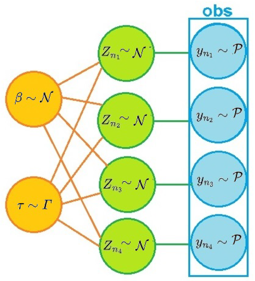
5. Numerical Experimentations of Normal–Poisson Distribution

The Normal–Poisson example is a non–conjugacy generalized mix model. The observed data are from a Poisson distribution named $y_n$ and a design vector $x_n$, for $n=1,\dots ,N$. The considered model is in Figure 1:

$$y_n|z_n\sim \mathcal{P}\left(exp\left(z_n\right)\right),$$

(16)

where

$$z_n|\beta ,\tau \sim \mathcal{N}\left(\beta x_n,{\tau }^{-1}\right),\beta \sim \mathcal{N}\left(\mathbf{0},{\mathit{\sigma }}_{\beta }^2\right),and\tau \sim \Gamma \left({\alpha }_{\tau },{\beta }_{\tau }\right).$$

In the first step, we approximate the posterior joint distribution of $\beta$, $\tau$ and $\mathit{z}=(z_1,\cdots ,z_n)$ for $n=1,\dots ,N$ via MFVBA:

$$q(\beta ,\tau ,\mathit{z})=q_{N+1}\left(\beta \right)q_{N+2}\left(\tau \right)\prod _{n=1}^N{q}_n\left(z_n\right).$$

We need to write $L=lnp(\beta ,\tau ,\mathit{z},y)$:

$$\begin{array}{cc}\hfill lnp(\beta ,\tau ,\mathit{z},y)=& -\frac{{\beta }^2}{2{\sigma }_{\beta }^2}+({\alpha }_{\tau }+\frac{N}{2}-1)ln\left(\tau \right)-{\beta }_{\tau }\tau -\frac{\tau }{2}\sum _{n=1}^N{z}_n^2-\frac{\tau {\beta }^2}{2}\sum _{n=1}^N{x}_n^2\hfill \\ \hfill & +\tau \beta \sum _{n=1}^N{z}_n{x}_n+\sum _{n=1}^N{z}_n{y}_n-\sum _{n=1}^{N}exp\left(z_n\right)-\sum _{n=1}^{N}ln(y_n!)+C,\hfill \end{array}$$

(17)

where C is a constant and does not depend on unknown variables. We start with computing the distributions of $z_n$ for $n=1,\dots ,N$. For the simplicity of notations, we assume that n is a natural number in the interval $[1,N]$, and $q_{N+2\setminus n}$ means all $N+2$ distribution items except the nth one, and ${\langle ·\rangle }_q$ means the expectation over density q. Thus, $q_n\left(z_n\right)$, the density of $z_n$, is equivalent to the following:

$$\begin{array}{c}\hfill {\langle lnp(\beta ,\tau ,\mathit{z},y)\rangle }_{q_{N+2\setminus n}}\propto -\frac{{\langle \tau \rangle }_{q_{N+2}}}{2}{z}_n^2+({\langle \tau \rangle }_{q_{N+2}}{\langle \beta \rangle }_{q_{N+1}}{x}_n+y_n)z_n-exp\left(z_n\right).\end{array}$$

Since this expression does not follow a specific distribution because of the existence of $exp\left(z_n\right)$, we omit this part according to its expectation, which is a function of ${\langle z_n\rangle }_{q_n}$ and ${\langle z_n^2\rangle }_{q_n}$. We can calculate the expectations using the Normal moment–generating distribution function. The logical reason is that its expectation depends only on ${\langle z_n\rangle }_{q_n}$ and ${\langle z_n^2\rangle }_{q_n}$. Moreover, we have ${\langle \tau \rangle }_{q_{N+2}}=\frac{{\alpha }_{\tau }}{{\beta }_{\tau }}$ and ${\langle \beta \rangle }_{q_{N+1}}=0$. Thus,

$$\begin{array}{c}\hfill {\langle lnp(\beta ,\tau ,\mathit{z},y)\rangle }_{q_{N+2\setminus n}}\propto -\frac{{\alpha }_{\tau }}{2{\beta }_{\tau }}\left(z_n^2-\frac{2{\beta }_{\tau }{y}_n}{{\alpha }_{\tau }}{z}_n\right),\end{array}$$

which means a Normal distribution for $z_n$, $\mathcal{N}(\frac{{\beta }_{\tau }{\overline{y}}_n}{{\alpha }_{\tau }},\frac{{\beta }_{\tau }}{{\alpha }_{\tau }})$ for $n=1,\dots ,N$. The process is quite similar for $q_{N+2}\left(\tau \right)$ and $q_{N+1}\left(\beta \right)$. The corresponding equivalents of distributions for $q_{N+2}$ and $q_{N+1}$ are shown below, respectively:

$$\begin{array}{cc}\hfill {\langle lnp(\beta ,\tau ,\mathit{z},y)\rangle }_{q_{1,\dots ,N+1}}\propto & ({\alpha }_{\tau }+\frac{N}{2}-1)ln\left(\tau \right)\hfill \\ \hfill & -\frac{\tau }{2}\left(2{\beta }_{\tau }+\sum _{n=1}^N({\langle z_n^2\rangle }_{q_n}+{\langle {\beta }^2\rangle }_{q_{N+1}}{x}_n^2-2{\langle \beta \rangle }_{q_{N+1}}{x}_n{\langle z_n\rangle }_{q_n})\right),\hfill \end{array}$$

and

$$\begin{array}{c}\hfill {\langle lnp(\beta ,\tau ,z,y)\rangle }_{q_{1,\dots ,N,N+2}}\propto -\frac{{\beta }^2}{2{\sigma }_{\beta }^2}-\frac{{\langle \tau \rangle }_{q_{N+2}}{\beta }^2}{2}\sum _{n=1}^N{x}_n^2+{\langle \tau \rangle }_{q_{N+2}}\beta \sum _{n=1}^N{\langle z_n\rangle }_{q_n}{x}_n.\end{array}$$

Thus, we have:

$$\begin{array}{c}\hfill \tau \sim \Gamma \left({\alpha }_{\tau }+\frac{N}{2},\frac{1}{2}\left(2{\beta }_{\tau }+\frac{{\beta }_{\tau }}{{\alpha }_{\tau }}N+\frac{{\beta }_{\tau }^2}{{\alpha }_{\tau }^2}\sum _{n=1}^N{\overline{y}}_n^2+{\sigma }_{\beta }^2\sum _{n=1}^N{x}_n^2\right)\right),\end{array}$$

and

$$\begin{array}{cc}\hfill \beta \sim \mathcal{N}& \left(\frac{{\sigma }_{\beta }^2(2{\alpha }_{\tau }+N)\frac{{\beta }_{\tau }}{{\alpha }_{\tau }}{\sum }_{n=1}^N{\overline{y}}_n{x}_n}{2{\beta }_{\tau }+\frac{{\beta }_{\tau }}{{\alpha }_{\tau }}N+\frac{{\beta }_{\tau }^2}{{\alpha }_{\tau }^2}{\sum }_{n=1}^N{\overline{y}}_n^2+{\sigma }_{\beta }^2(2{\alpha }_{\tau }+N+1){\sum }_{n=1}^N{x}_n^2},\right.\hfill \\ \hfill & \left.\frac{{\sigma }_{\beta }^2\left(2{\beta }_{\tau }+\frac{{\beta }_{\tau }}{{\alpha }_{\tau }}N+\frac{{\beta }_{\tau }^2}{{\alpha }_{\tau }^2}{\sum }_{n=1}^N{\overline{y}}_n^2+{\sigma }_{\beta }^2{\sum }_{n=1}^N{x}_n^2\right)}{2{\beta }_{\tau }+\frac{{\beta }_{\tau }}{{\alpha }_{\tau }}N+\frac{{\beta }_{\tau }^2}{{\alpha }_{\tau }^2}{\sum }_{n=1}^N{\overline{y}}_n^2+{\sigma }_{\beta }^2(2{\alpha }_{\tau }+N+1){\sum }_{n=1}^N{x}_n^2}\right).\hfill \end{array}$$

In the second step, we calculate the variance diagonal matrix $\mathit{V}$:

$$\mathit{V}=\left[\begin{array}{ccc}{\Sigma }_{\beta }& 0& 0\\ 0& {\Sigma }_{\tau }& 0\\ 0& 0& {\mathbf{\Sigma }}_{\mathit{z}}\end{array}\right],$$

where

$$\begin{array}{cc}\hfill {\Sigma }_{\beta }=& \frac{{\sigma }_{\beta }^2\left(2{\beta }_{\tau }+\frac{{\beta }_{\tau }}{{\alpha }_{\tau }}N+\frac{{\beta }_{\tau }^2}{{\alpha }_{\tau }^2}{\sum }_{n=1}^N{\overline{y}}_n^2+{\sigma }_{\beta }^2{\sum }_{n=1}^N{x}_n^2\right)}{2{\beta }_{\tau }+\frac{{\beta }_{\tau }}{{\alpha }_{\tau }}N+\frac{{\beta }_{\tau }^2}{{\alpha }_{\tau }^2}{\sum }_{n=1}^N{\overline{y}}_n^2+{\sigma }_{\beta }^2(2{\alpha }_{\tau }+N+1){\sum }_{n=1}^N{x}_n^2},\hfill \\ \hfill {\Sigma }_{\tau }=& \frac{2(2{\alpha }_{\tau }+N)}{{\left(2{\beta }_{\tau }+\frac{{\beta }_{\tau }}{{\alpha }_{\tau }}N+\frac{{\beta }_{\tau }^2}{{\alpha }_{\tau }^2}{\sum }_{n=1}^N{\overline{y}}_n^2+{\sigma }_{\beta }^2{\sum }_{n=1}^N{x}_n^2\right)}^2},\hfill \end{array}$$

and

$$\begin{array}{c}\hfill {\Sigma }_{z_n}=\frac{{\beta }_{\tau }}{{\alpha }_{\tau }},n=1,\dots ,N.\end{array}$$

Thus, ${\mathbf{\Sigma }}_z=diag({\Sigma }_{z_1},\cdots ,{\Sigma }_{z_N})$. The third step is to compute the Hessian matrix $\mathit{H}$:

$$\mathit{H}=\left[\begin{array}{ccc}\frac{{\partial }^{2}L}{\partial {\beta }^2}& \frac{{\partial }^{2}L}{\partial \beta \partial \tau }& \frac{{\partial }^{2}L}{\partial \beta \partial \mathit{z}}\\ \frac{{\partial }^{2}L}{\partial \tau \partial \beta }& \frac{{\partial }^{2}L}{\partial {\tau }^2}& \frac{{\partial }^{2}L}{\partial \tau \partial \mathit{z}}\\ \frac{{\partial }^{2}L}{\partial \mathit{z}\partial \beta }& \frac{{\partial }^{2}L}{\partial \mathit{z}\partial \tau }& \frac{{\partial }^{2}L}{\partial {\mathit{z}}^2}\end{array}\right].$$

Since $\mathit{H}$ is symmetric in our case study, we need to calculate the main diagonal and the upper triangle. This covariance matrix depends on the values of $\mathit{m}$:

$$\begin{array}{c}\hfill \mathit{m}={\left(E_q\left(\beta \right),E_q\left({\beta }^2\right),E_q\left(\tau \right),E_q(ln\left(\tau \right)),E_q\left(z_1\right),E_q\left(z_1^2\right),\dots ,E_q\left(z_N\right),E_q\left(z_N^2\right)\right)}^T.\end{array}$$

Thus, the diagonal of $\mathit{H}$ as a function of $\mathit{m}$ is shown below:

$$\begin{array}{cc}\hfill \frac{{\partial }^{2}L}{\partial {\beta }^2}=& -\frac{1}{{\sigma }_{\beta }^2}-E_q\left(\tau \right)\sum _{n=1}^N{x}_n^2,\hfill \\ \hfill \frac{{\partial }^{2}L}{\partial {\tau }^2}=& -({\alpha }_{\tau }+\frac{N}{2}-1)E_q\left(\frac{1}{{\tau }^2}\right),\hfill \\ \hfill \frac{{\partial }^{2}L}{\partial z_n^2}=& -E_q\left(\tau \right)-E_q(exp\left(z_n\right)),n=1,\dots ,N,\hfill \end{array}$$

where L is defined in Equation (17). The upper triangle is:

$$\begin{array}{cc}\hfill \frac{{\partial }^{2}L}{\partial \beta \partial \tau }=& -E_q\left(\beta \right)\sum _{n=1}^N{x}_n^2+\sum _{n=1}^N{E}_q\left(z_n\right)x_n,\hfill \\ \hfill \frac{{\partial }^{2}L}{\partial \beta \partial z_n}=& E_q\left(\tau \right)x_n,n=1,\dots ,N,\hfill \\ \hfill \frac{{\partial }^{2}L}{\partial \tau \partial z_n}=& -E_q\left(z_n\right)+E_q\left(\beta \right)x_n,n=1,\dots ,N.\hfill \end{array}$$

The last step is to compute $\mathbf{\Sigma }$ using (15). For numerical experimentation, we generate data from the Normal–Poisson model with these descriptions:

$${\sigma }_{\beta }^2=10,{\alpha }_{\tau }=1,{\beta }_{\tau }=1,N=4.$$

We generate $x_n$ for $n=1,\dots ,N$ from the Normal distribution $\mathcal{N}(2,1)$. The number of the reputation for vector $y_n$ is 100, so $y_n$ is a matrix $N\times 100$. The only data we use are the observation matrix $y_n$ and vector $x_n$. The covariance matrix $\mathit{V}$ from MFVBA is a diagonal matrix:

$$\mathit{V}=\left[\begin{array}{ccc}1.48927& 0& {\mathbf{0}}^T\\ 0& 0.00071& {\mathbf{0}}^T\\ \mathbf{0}& \mathbf{0}& \mathit{I}\end{array}\right],$$

where $\mathbf{0}$ and $\mathit{I}$ are the zero vector with N dimensions and the identity matrix with $N\times N$ dimensions, respectively. The Hessian matrix $\mathit{H}$ and matrix $\mathit{I}-\mathit{V}\mathit{H}$ are:

$$\mathit{H}=\left[\begin{array}{cccccc}-0.67147& 0.09617& 0.05557& 0.03031& 0.13360& 0.07026\\ 0.09617& -1639.9471& -0.21738& -0.02130& 0.02651& 0.06653\\ 0.05557& -0.21738& -2.20665& 0& 0& 0\\ 0.03031& -0.02130& 0& -1.78014& 0& 0\\ 0.13360& 0.02651& 0& 0& -1.86901& 0\\ 0.07026& 0.06653& 0& 0& 0& -1.69561\end{array}\right],$$

and

$$\mathit{I}-\mathit{V}\mathit{H}=\left[\begin{array}{cccccc}2& -0.14322& -0.08276& -0.04514& -0.19897& -0.10464\\ -6.8318{ \times 10}^{-5}& 2.16501& 0.00015& 1.5130{ \times 10}^{-5}& -1.8832{ \times 10}^{-5}& -4.7264{ \times 10}^{-5}\\ -0.05557& 0.21738& 3.20665& 0& 0& 0\\ -0.03031& 0.02130& 0& 2.78014& 0& 0\\ -0.13360& -0.02651& 0& 0& 2.86901& 0\\ -0.07026& -0.06653& 0& 0& 0& 2.69561\end{array}\right].$$

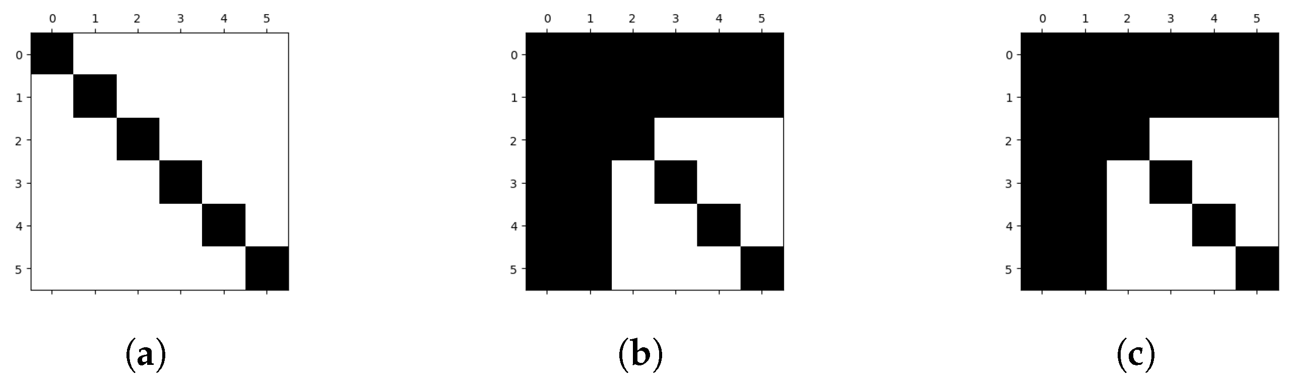
The covariance matrix via LRVBA is:

$$\mathbf{\Sigma }=\left[\begin{array}{cccccc}0.74986& 2.3409{ \times 10}^{-5}& 0.01299& 0.00818& 0.03492& 0.01955\\ 2.3408{ \times 10}^{-5}& 0.00033& -2.1838{ \times 10}^{-5}& -2.2586{ \times 10}^{-6}& 4.1220{ \times 10}^{-6}& 8.7090{ \times 10}^{-6}\\ 0.01299& -2.1838{ \times 10}^{-5}& 0.31208& 0.00014& 0.00060& 0.00034\\ 0.00817& -2.2586{ \times 10}^{-6}& 0.00014& 0.35978& 0.00038& 0.00021\\ 0.03492& 4.1220{ \times 10}^{-6}& 0.00060& 0.00038& 0.35018& 0.00091\\ 0.01955& 8.7090{ \times 10}^{-6}& 0.00034& 0.00021& 0.00091& 0.37148\end{array}\right].$$

(18)

The sparsity patterns for the $\mathit{V}$, $\mathit{H}$ and $\mathit{I}-\mathit{V}\mathit{H}$ matrixes are shown in Figure 2.

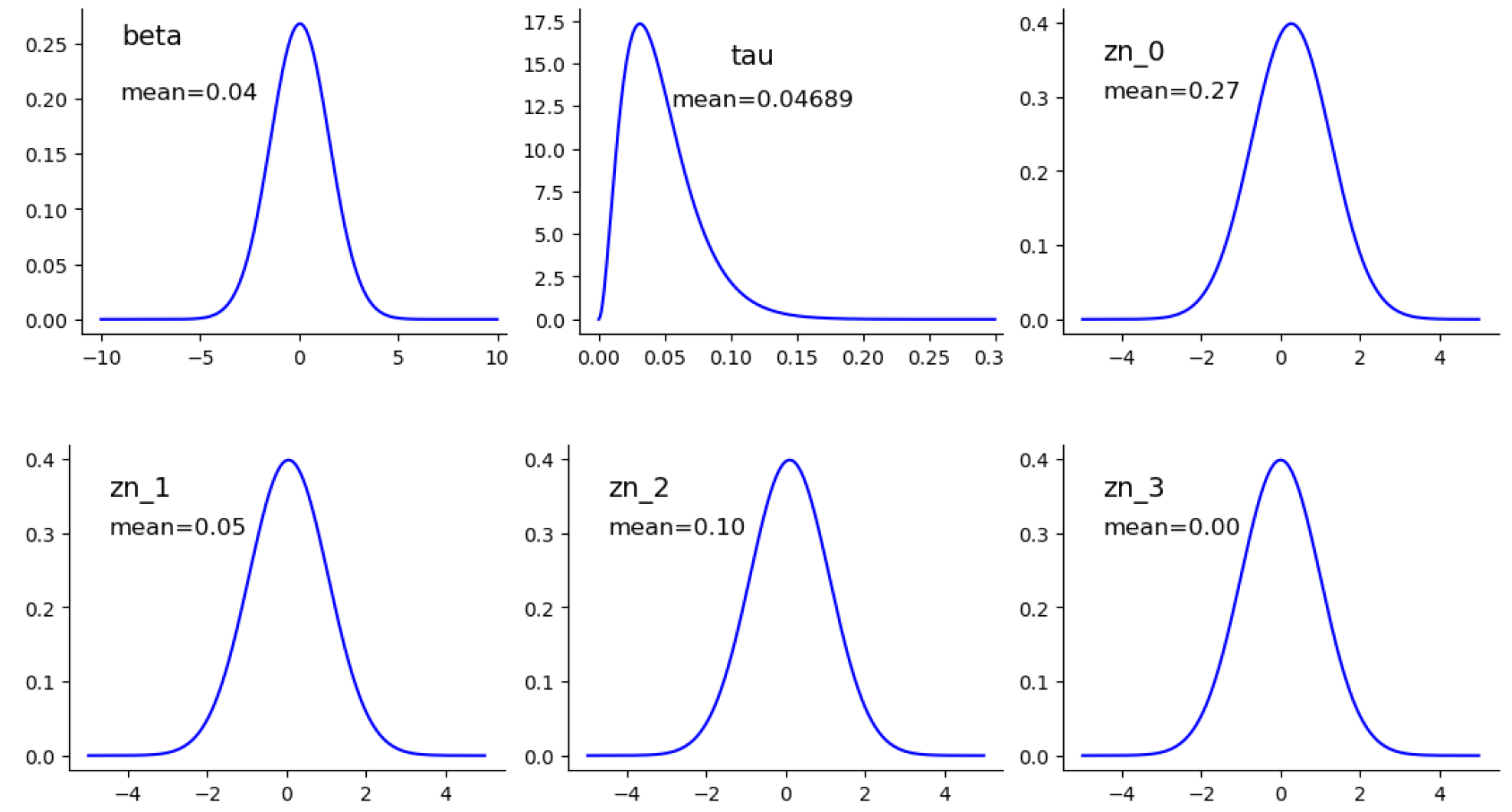
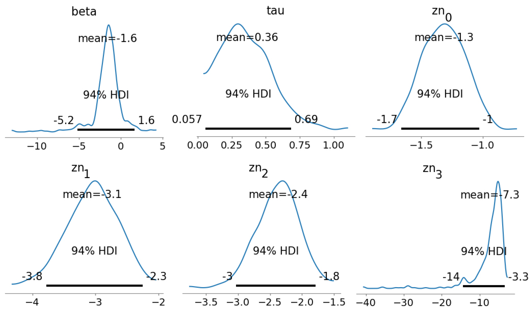
In addition, we simulate the posterior distribution via MCMC. This simulation has five chains and one divergence. The estimated marginal distribution for each unknown variable is shown in Figure 3 and Figure 4 via MFVBA and MCMC, respectively. More details are in

Table 1. Summary of the margin densities for unknown variables.

Unknown	MFVBA Method		LRVBA Method	MCMC Method
	mean	sd	sd	mean	sd	hdi–3%	hdi–97%	MCSE–mean	MCSE–sd	ess–bulk	ess–tail	r–hat
$\beta$	$0.044$	$1.220$	$0.866$	$-1.616$	$1.769$	$-5.175$	$1.620$	$0.148$	$0.194$	$186.0$	$43.0$	$1.11$
$\tau$	$0.047$	$0.027$	$0.018$	$0.361$	$0.188$	$0.057$	$0.685$	$0.024$	$0.017$	$38.0$	$51.0$	$1.11$
$z_0$	$0.270$	1	$0.559$	$-1.316$	$0.177$	$-1.664$	$-1.028$	$0.008$	$0.006$	$468.0$	$316.0$	$1.02$
$z_1$	$0.050$	1	$0.600$	$-3.051$	$0.410$	$-3.783$	$-2.252$	$0.021$	$0.015$	$382.0$	$372.0$	$1.00$
$z_2$	$0.100$	1	$0.592$	$-2.375$	$0.332$	$-3.029$	$-1.790$	$0.015$	$0.011$	$476.0$	$415.0$	$1.02$
$z_3$	0	1	$0.610$	$-7.334$	$4.641$	$-14.366$	$-3.311$	$0.868$	$0.620$	$45.0$	$55.0$	$1.13$

. The joint distribution of unknown variables is approximated via MFVBA and MCMC. The MFVBA distribution is the marginal density factorial of the unknown variables. Therefore, the variables are independent in MFVBA, and the covariance matrix is diagonal. LRVBA is a correction method on the covariance matrix. Thus, the matrix is no longer diagonal as presented in (18). Also, we add more details about the MCMC results in Table 1. The Monte Carlo Standard Error (MCSE) is a chain–accurate measure and provides a quantitative suggestion of how big the estimation noise is. The noises are small based on the mean and sd of the MCSE. The ess–bulk column delivers an evaluated bulk influential sample size using rank–normalised draws. The ess–tail column creates an approximated tail practical sample size by computing the effective minimum sample sizes between the $5\%$ and $95\%$ quantiles. The last column is the r–hat convergence diagnostic, which compares the between and within–chain estimation for model variables and other univariate quantities.

6. Conclusions

Bayesian computations are used to infer unknown parameters from data. ABC methods are applied to perform approximate computation, particularly in high–dimensional problems. Two classes of approximate computational methods are MCMC and VBA. MCMC generates samples from the probability function to approximate the posterior distribution. It generates a sequence of samples that converges to the target distribution. The VBA approximates the expression of the joint posterior distribution of unknown parameters in a complex model using a simple expression. VBA has some advantages over MCMC, such as being faster, more scalable and versatile. It also guarantees convergence to a local minimum of KL divergence.

VBA’s drawback is that it underestimates the covariance matrix of the unknowns. For this aim, we use LRVB to approximate the covariance more precisely. However, the LRVB computations still need the inversion of some matrixes, which is costly when the unknown parameters’ dimensions are high. We work on a numerical example to show the whole process of VBA and LRVB as well as the performance and ability of the proposed method and compare it with the classical MCMC results. As a result of the numerical example, the VBA implementation was much shorter than the MCMC, and we had an explicit form of joint distribution with a modified covariance matrix with the LRVB aid.

References

1. Metropolis, N.; Rosenbluth, A.W.; Rosenbluth, M.N.; Teller, A.H.; Teller, E. Equation of state calculations by fast computing machines. J. Chem. Phys. 1953, 21, 1087–1092. [Google Scholar] [CrossRef]
2. Hastings, W.K. Monte Carlo sampling methods using Markov chains and their applications. Biometrika 1970, 57, 97–109. [Google Scholar] [CrossRef]
3. Jordan, M.I.; Ghahramani, Z.; Jaakkola, T.S.; Saul, L.K. An introduction to variational methods for graphical models. In Learning in Graphical Models; Springer: Dordrecht, The Netherlands, 1998; pp. 105–161. [Google Scholar]
4. Sarkka, S.; Nummenmaa, A. Recursive noise adaptive Kalman filtering by variational Bayesian approximations. IEEE Trans. Autom. Control 2009, 54, 596–600. [Google Scholar] [CrossRef]
5. Rohde, D.; Wand, M.P. Semiparametric mean field variational Bayes: General principles and numerical issues. J. Mach. Learn. Res. 2016, 17, 5975–6021. [Google Scholar]
6. Giordano, R.J.; Broderick, T.; Jordan, M.I. Linear response methods for accurate covariance estimates from mean field variational Bayes. Adv. Neural Inf. Process. Syst. 2015, 28, 1441–1449. [Google Scholar]
7. Giordano, R.; Broderick, T.; Jordan, M.I. Covariances, robustness and variational bayes. J. Mach. Learn. Res. 2018, 19, 1–49. [Google Scholar]
Figure 1. The Normal–Poisson hierarchical model pattern when N = 4 with sample size 100.
Psf 09 00012 g001
Figure 2. Sparsity patterns for the matrices using model (16). (a) VBA covariance matrix V ; (b) Hessian matrix H ; (c) I V H matrix.
Psf 09 00012 g002
Figure 3. The final estimations of margin densities for each variable via MFVBA method.
Psf 09 00012 g003
Figure 4. The final margins via MCMC method.
Psf 09 00012 g004