1. Introduction
Inverse problems arise almost everywhere in science and engineering. In fact, anytime and in any application when we have indirect measurements related to what we really want to measure through some mathematical relation, this is called the forward model. Then, we have to infer the desired unknown from the observed data using this forward model or a surrogate one. In general, many inverse problems are ill-posed, and many methods for finding well-posed solutions for them are mainly based either on regularization theory or Bayesian inference. We mention those in particular, which are based on the optimization of a criterion with two parts: a data model output matching criterion (likelihood part in the Bayesian) and a regularization term (prior model in the Bayesian). Different criteria for these two terms and a great number of standard and advanced optimization algorithms have been proposed and used with great success. When these two terms are distances, they can have a Bayesian maximum a posteriori (MAP) interpretation, where these two terms correspond, respectively, to the likelihood and prior probability models. The Bayesian approach gives more flexibility in choosing these terms via the likelihood and the prior probability distributions. This flexibility goes much further with the hierarchical models and appropriate hidden variables [
1]. Also, the possibility of estimating the hyperparameters gives much more flexibility for semisupervised methods.
However, full Bayesian computations can become very heavy computationally. In particular, this occurs when the forward model is complex, and the evaluation of the likelihood has a high computational cost [
2]. In those cases, using surrogate simpler models can become very helpful to reduce the computational costs, but then we have to account for the uncertainty quantification (UQ) of the obtained results [
3]. Neural networks (NNs), with their diversity such as convolutional neural networks (CNNs), deep learning (DL), etc., have become tools for fast and low computational surrogate forward models.
Over the last decades, machine learning (ML) methods and algorithms have gained great success in many tasks, such as classification, clustering, segmentation, object detection, and many other areas. There are many different structures of neural networks (NNs), such as feed-forward, Convolutional NNs (CNNs), Deep NNs, etc. [
4]. Using these methods directly for inverse problems, as intermediate preprocessing or as tools for performing fast approximate computation in different steps of regularization or Bayesian inference, has also been successful, but not as much as could be possible. Recently, physics-informed neural networks have gained great success in many inverse problems, thereby proposing interaction between the Bayesian formulation of forward models and optimization algorithms and ML-specific algorithms for intermediate hidden variables. These methods have become very helpful to obtain approximate practical solutions to inverse problems in real-world applications [
5,
6,
7,
8,
9,
10,
11].
In this paper, first, in
Section 2, some mathematical notations for dealing with NNs are given. In
Section 3, a detailed presentation of the Bayesian inference and the approximate computation needed for BDL are given. Then, in
Section 4, we consider a focus on the NN and DL methods for inverse problems. First, we present the same cases where we know the forward and its adjoint model. Then, we consider the case where we may not have this knowledge and want to propose directly data-driven DL methods [
12,
13].
2. Neural Networks, Deep Learning, and Bayesian DL
The main objective of the NN for a regression problem can be described as follows:
The objective is to infer the function
from the observations
at locations given by
. The usual NN learning approach is to define a parametric family of functions
that is flexible enough so that
such that
:
Deep learning focuses on learning the optimal parameters
, which can then be used for predicting the output
for any input
:
In this approach, there is no uncertainty quantification.
The Bayesian deep learning approach can be summarized as follows:
As we can see, uncertainties are accounted for in both steps of the parameter estimation and prediction. However, as we will see, the computational costs are important. We need to find solutions to perform fast computation.
3. Bayesian Inference and Approximate Computation
In a general Bayesian framework for NNs and DL, the objective is to infer the parameters
from the data,
, using the Bayes rule:
where
is the prior,
is the likelihood,
is the posterior, and
is called the evidence. We can also write
, where the classical maximum likelihood estimation (MLE) is defined as
.
A particular point of the posterior is of high interest, because we may be interested in maximum a posterior (MAP) estimation: . We may also be interested in mean squared error (MSE) estimation, which is shown that it corresponds to .
The exact expression of the posterior and the computations of these integrals for great dimensional problems may be very computationally costly. For this reason, we need to perform approximate computation. In the following subsections, we review a few solutions.
3.1. Laplace Approximation
Rewriting the general Bayes rules slightly differently gives us the following:
the Laplace approximations use a second-order expansion of
around
to construct a Gaussian approximation of
:
where the first-order term vanishes at the
. This is equivalent to calculating the following approximation:
With this approximation, the evidence
is approximated by the following:
For great dimensional problems such as BDL, the full computation of is very costly. We have still to do more approximations. The following are a few solutions for scalable approximations for BDL:
Work with the subnetwork or last layer (transfer learning);
Perform covariance matrix decomposition (low rank, Kronecker-factored approximate curvature (KFAC), Diag);
Conduct the computation during the hyperparameter tuning using crossvalidation;
Use approximate predictive computation.
3.2. Approximate Computation: Variational Inference
The main idea then is to perform approximate Bayesian computation (ABC) by approximating the posterior
using a simpler expression
. When approximation is performed by minimizing
the method is called the variational Bayesian approximation (VBA). When
is chosen to be separable in some components of the parameters
, the approximation is called
the mean field VBA (MFVBA).
Let us come back to the general VBA,
, and note using
the expected likelihood and using
the entropy of
q. Then, we have the following:
E is also called the evidence lower bound (ELBO):
At this point, it is important to note one main property of the VBA: When
, the posterior probability law
p and the approximate probability law
q are in the exponential family; then,
.
3.3. VBA and Natural Exponential Family
If
q is chosen to be in a
natural exponential family,
, then it is entirely characterized by its mean
, and if
q is conjugate to
p, then
, which is entirely characterized by its mean
. We can then define the objective
E as a function of
, and the first order condition of the optimality is
. From this property, we can obtain a fixed-point algorithm to compute
:
Iterating on this
fixed-point algorithm gives us the following:
which converges to
and is also
. This algorithm can be summarized as follows:
Having chosen the prior and likelihood, find the expression of ;
Choose a family q and find the expressions of and , which thus yield as a function of ;
Find the expression of the vector operator and update it until convergence, which results in .
At this point, it is important to note that, in this approach, even if the mean is well approximated, the variances or the covariance are underestimated. Some authors who are interested in this approach have proposed solutions to better estimate the covariance. See [
14] for one of the solutions.
4. Deep Learning and Bayesian DL
As introduced before, in classical DL, the training and prediction steps can be summarized as follows:
In this approach, there is no uncertainty quantification. The Bayesian deep learning can be summarized as follows:
As we can see, uncertainties are accounted for in both steps of the parameter estimation and prediction. However, computational costs are important. We need to find solutions to perform fast computation. As mentioned before, the different possible tools are Laplace and Gaussian approximation, variational inference, and more controlled approximation to design new deep learning algorithms, which can scale up for practical situations.
Exponential Family Approximation
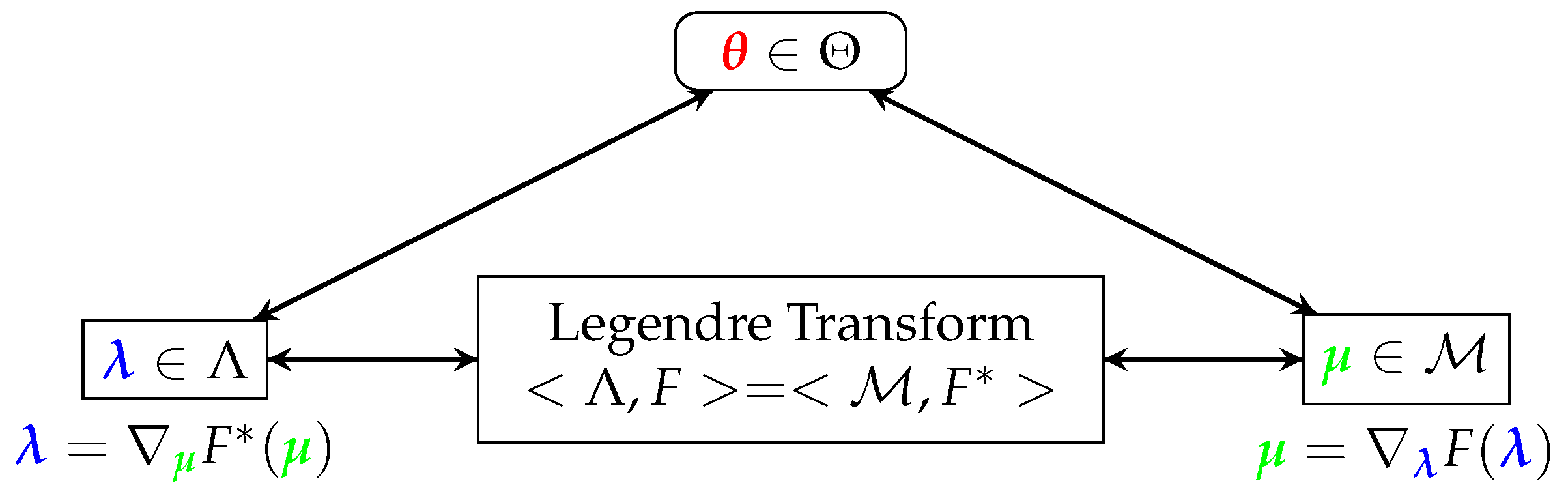
Let us consider the case of general exponential families
, where
represents the original parameters,
represents the natural parameters,
represents sufficient statistics,
represents the log partition function, and we define the expectations parameters as
. Let us also define the dual function
and the dual parameters
via the Legendre transform:
Then, we can show the triangular relation between
,
, and
shown in
Figure 1.
With these notations, applying the VBA rule
results in the following updating rule for the natural parameters:
For example, by considering the Gaussian case
we can identify the natural parameters as
, and we easily obtain the following algorithm:
where
which results, explicitly, in
For a linear model
and Gaussian priors, we have
and
.
It is interesting to note that many classical algorithms for updating the parameters, such as forward–backward, sparse variational inference, and variational message passing, become special cases. A main remark here is that this linear generating function case will link us to the linear inverse problems if we replace with , with , and with .
5. NN, DL, and Bayesian Inference for Linear Inverse Problems
To show the possibilities of the interaction between inverse problems methods, neural networks and deep learning, the best way is to give a few examples.
5.1. First Example: A Known Linear Forward Model
The first and easiest example is the case of linear inverse problems
, where we know the forward model
and we assume the Gaussian likelihood
and the Gaussian prior
are the easiest cases to consider, where we know that the posterior is Gaussian
with
where
,
,
,
, and
.
These relations can be presented schematically as
We can then consider replacing
,
, and
with appropriate deep neural networks and apply all the previous BDL methods to them. As we can see, these relations directly induce a linear feed-forward NN structure. In particular, if
represents a convolution operator, then
,
, and
are too, as well as the operators
and
. Thus, the whole inversion can be modeled using a CNN [
15,
16].
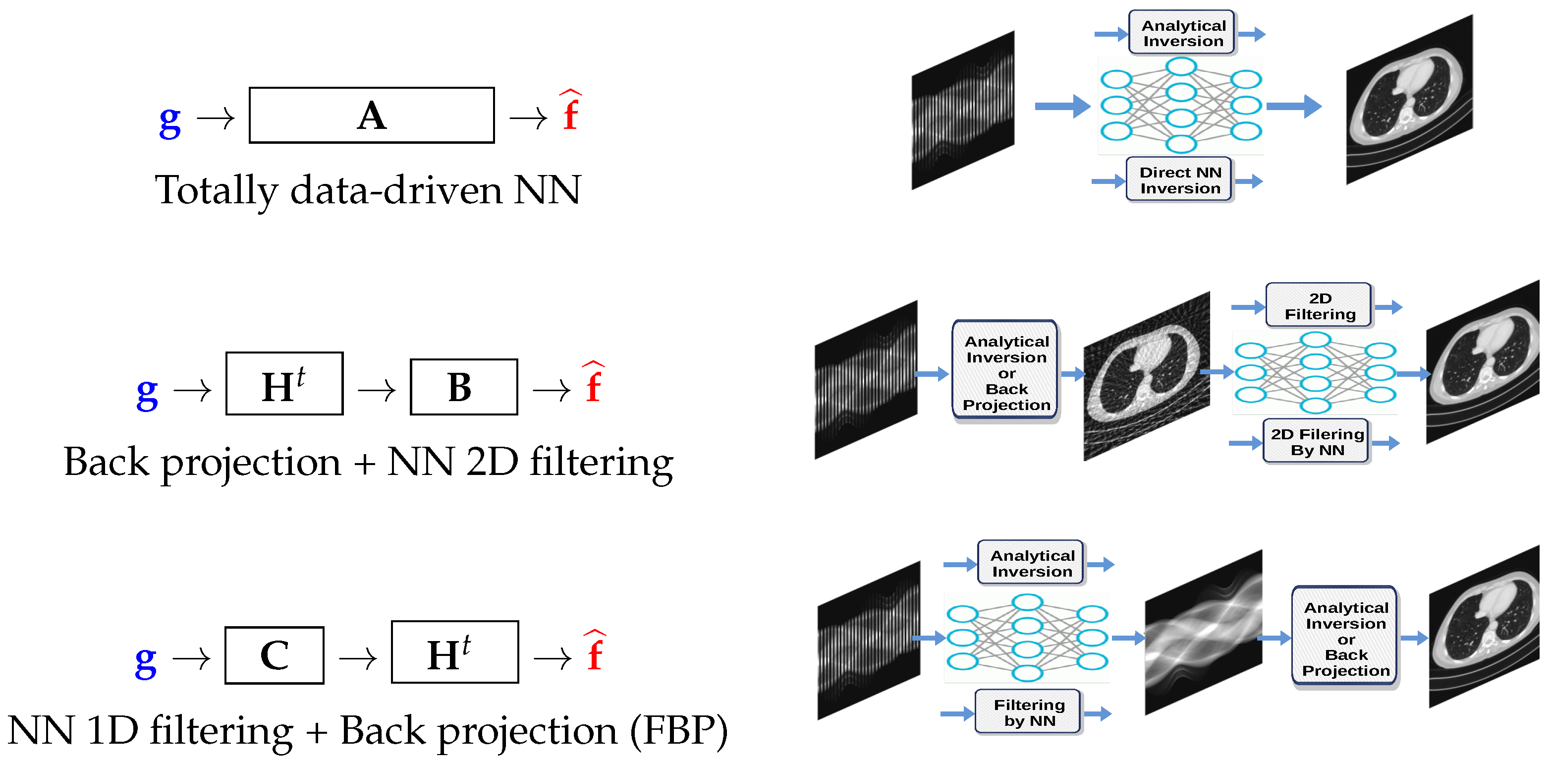
For the case of computed tomography (CT), the first operation is equivalent to an analytic inversion, the second corresponds to back projection that is first followed by 2D filtering in the image domain, and the third corresponds to the famous filtered back projection (FBP), which is implemented on classical CT scans. These cases are illustrated in
Figure 2.
5.2. Second Example: A Deep Learning Equivalence of Iterative Gradient-Based Algorithms
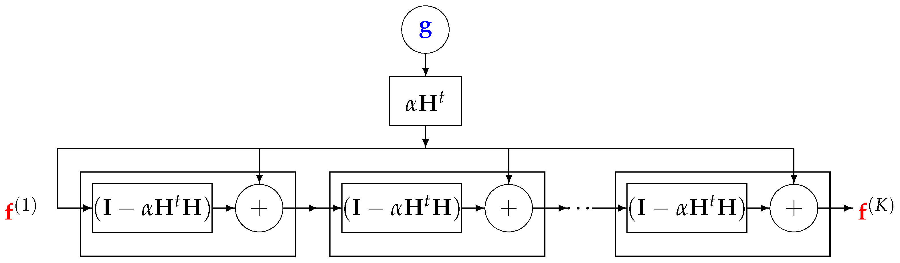
One of the classical iterative methods in linear inverse problem algorithms is based on the gradient descent method to optimize
:
where the solution to the problem is obtained recursively. Everybody knows that when the forward model operator
is singular or ill-conditioned, this iterative algorithm starts by converging, but it may diverge easily. One of the experimental methods to obtain an acceptable approximate solution is just to stop the iterations after
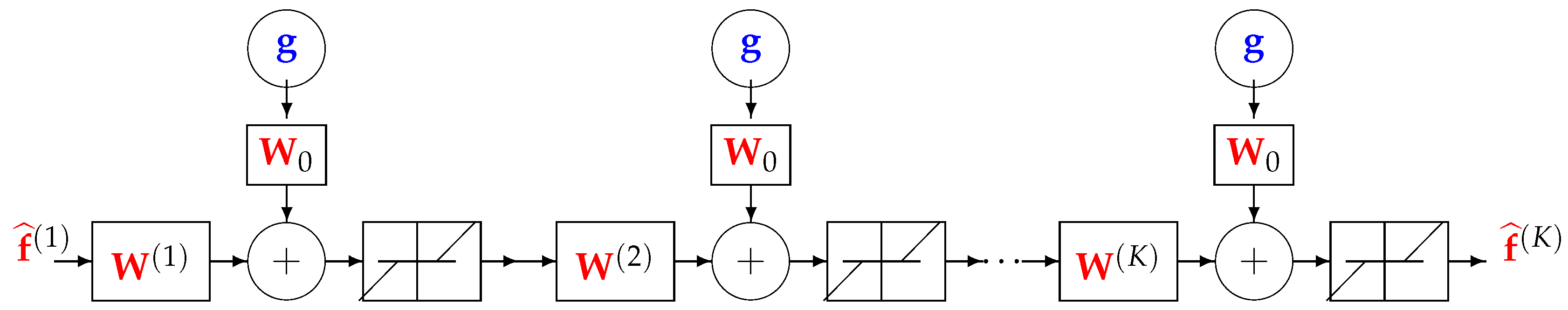
K iterations. This idea can be translated to a deep learning NN by using
K layers. Each layer represents one iteration of the algorithm. See
Figure 3.
This DL structure can easily be extended to a regularized criterion.
, which can also be interpreted as the MAP or posterior mean solution with a Gaussian likelihood and prior. In this case, we have the following:
We just need to replace
with
.
This structure can also be extended to all the sparsity-enforcing regularization terms such as and the total variation (TV) using appropriate algorithms such as the ISTA (iterative soft threshold algorithm) or its fast version FISTA by replacing the update expression and by adding an NL operation, much like the ordinary NNs. A simple example is given in the following subsection.
5.3. Third Example: Regularization and NN
The case of the MAP solution with a Gaussian likelihood and double exponential prior becomes equivalent to the
regularization criterion:
where the solution can be obtained with an iterative optimization algorithm, such as ISTA:
where
is a soft threshold operator, and
is the Lipschitz constant of the normal operator. When
is a convolution operator, then
Using the iterative gradient-based algorithm with a fixed number of iterations for computing a GI or a regularized one, as explained in the previous section, can be used to propose a DL structure with
K layers, with
K being the number of iterations before stopping.
Figure 5 shows this structure for a quadratic regularization, which results in a linear NN, and
Figure 6 shows the case of
regularization.
In all these examples, we could directly obtain the structure of the NN from the forward model and known parameters. However, in these approaches, there are some difficulties that consist of the determination of the structure of the NN. For example, in the first example, obtaining the structure of
depends on the regularization parameter
. The same difficulty arises in determining the shape and the threshold level of the threshold bloc of the network in the second example. The same need for the regularization parameter, as well as many other hyperparameters, makes it necessary to create the NN structure and weights. In practice, we can decide, for example, on the number and structure of a DL network, but as their corresponding weights depend on many unknown or difficult-to-fix parameters, ML may become of help. In the following, we first consider the training part of a general ML method. Then, we will see how to include the physics-based knowledge of the forward model in the structure of learning [
4,
10,
17,
18].
5.4. Decomposition of the NN Structure to Fixed and Trainable Parts
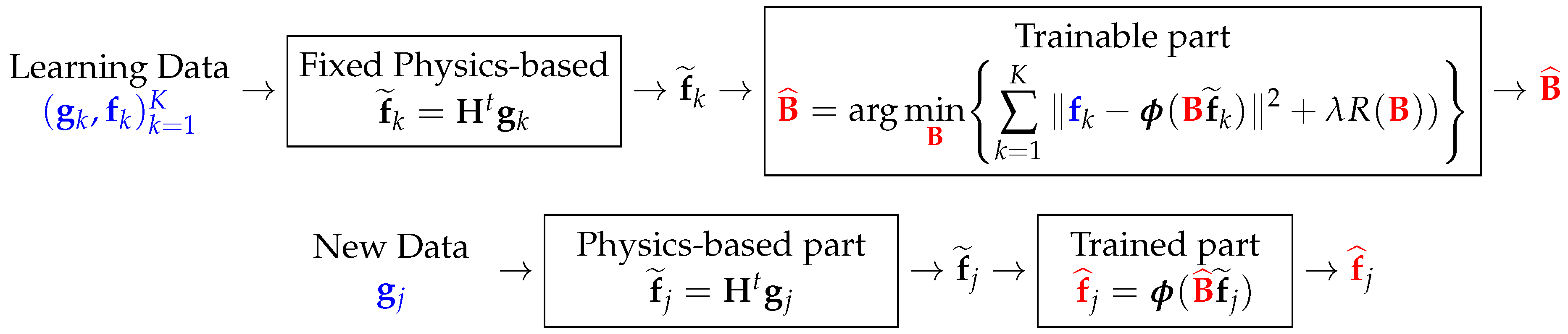
The first easiest and most understandable method consists of decomposing the structure of the network
in two parts: a fixed part and a learnable part. As the simplest example, we can consider the case of analytical expression of the quadratic regularization
, which suggests having a two-layer network with a fixed part structure
and a trainable one
. See
Figure 6.
It is interesting to note that in X-ray-computed tomography (CT), the forward operator is called projection, the adjoint operator is called back projection (BP), and the operator is assimilated to a 2D filtering (convolution).
6. DL Structure and Deterministic or Bayesian Computation
To be able to look at the DNN and analyze it either in a deterministic or Bayesian manner, let us come back to the general notations and consider the following NN with input
, output
, and intermediate hidden variables
:
In the deterministic case, each layer is defined by its parameters
:
and we can write:
with
and
6.1. Deterministic DL Computation
In general, during the training steps, the parameters
are estimated via
The main point here is to choose how to choose
and
, as well as which optimization algorithm to choose for better convergence.
When parameters are obtained (the model is trained), we can use it easily via
6.2. Bayesian Deep Neural Network
In Bayesian DL, the question of choosing and in the previous case becomes the choice of the prior, , which can also be assumed to be a priori separable in the components of or not. Then, we have to choose the expression of the likelihood (in general Gaussian) and find the expression of the posterior . As explained extensively before, directly using this posterior is almost impossible. Hopefully, we have a great number of approximate computation methods, such as MCMC sampling, slice sampling, nested sampling, data augmentation, and variational inference, which can still be used in practical situations. However, the training step in the Bayesian DL still stays very costly, particularly if we want to quantify the uncertainties.
Prediction Step
In the prediction step, we again have to consider choosing a probability law
for the class of the possible inputs and for all the outputs
that are conditional to their inputs
. Then, we can consider, for example, the Gibbs sampling scheme. A comparison between deterministic and Bayesian DL is shown here:
If we consider Gaussian laws for the input and all the conditional variables, then we can write the following:
Here too, the main difficulty occurs when there are nonlinear activation functions, particularly in the last layer, where the Gaussian approximation may not be more valid.
7. Application: Infrared Imaging
Infrared (IR) imaging is used to diagnose and to survey the temperature field distribution of sensitive objects in many industrial applications. These images are, in general, low resolution and very noisy. The real values of the temperature also depend on many other parameters, such as emissivity, attenuation, and diffusion, due to the distance of the camera to the sources. To be really useful in practice, we need to reduce the noise, calibrate and increase the resolution, segment for detection of the hot area, and finally survey the temperature values of the different areas during the time to be able to conduct preventive diagnosis and possible maintenance.
Reducing the noise can be accomplished by filtering using the Fourier transform, wavelet transform, or other sparse representations of images. To increase the resolution, we may use deconvolution methods if we can obtain the point spread function (PSF) of the camera, or if not by using blind deconvolution techniques. The segmentation and detection of the hot area and the temperature value estimation at each area are also very important steps in real applications. Any of these steps can be performed separately, but trying to propose global processing using DL or BDL is necessary for real applications. As any of these steps are in fact different inverse problems, and it is difficult to fix the parameters in each step in a robust way, we propose a global process using the BDL. See the global scheme in
Figure 7.
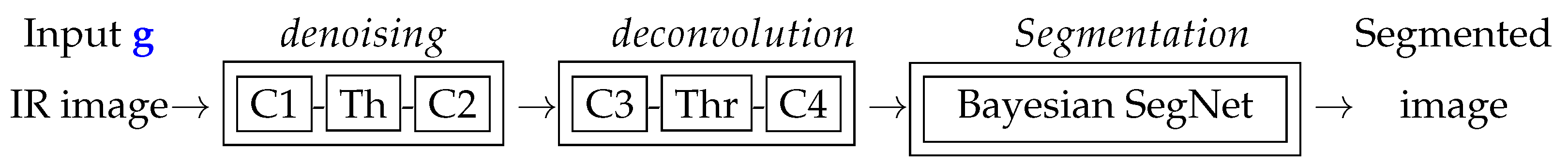
In the first step, as the final objective is to segment the image to obtain different levels of temperature (for example, four levels: background, normal, high, and very high), we propose to design an NN that obtains as input a low resolution and noisy image and outputs a segmented image with those four levels and, at the same time, a good estimate of the temperature at each segment. See
Figure 8.
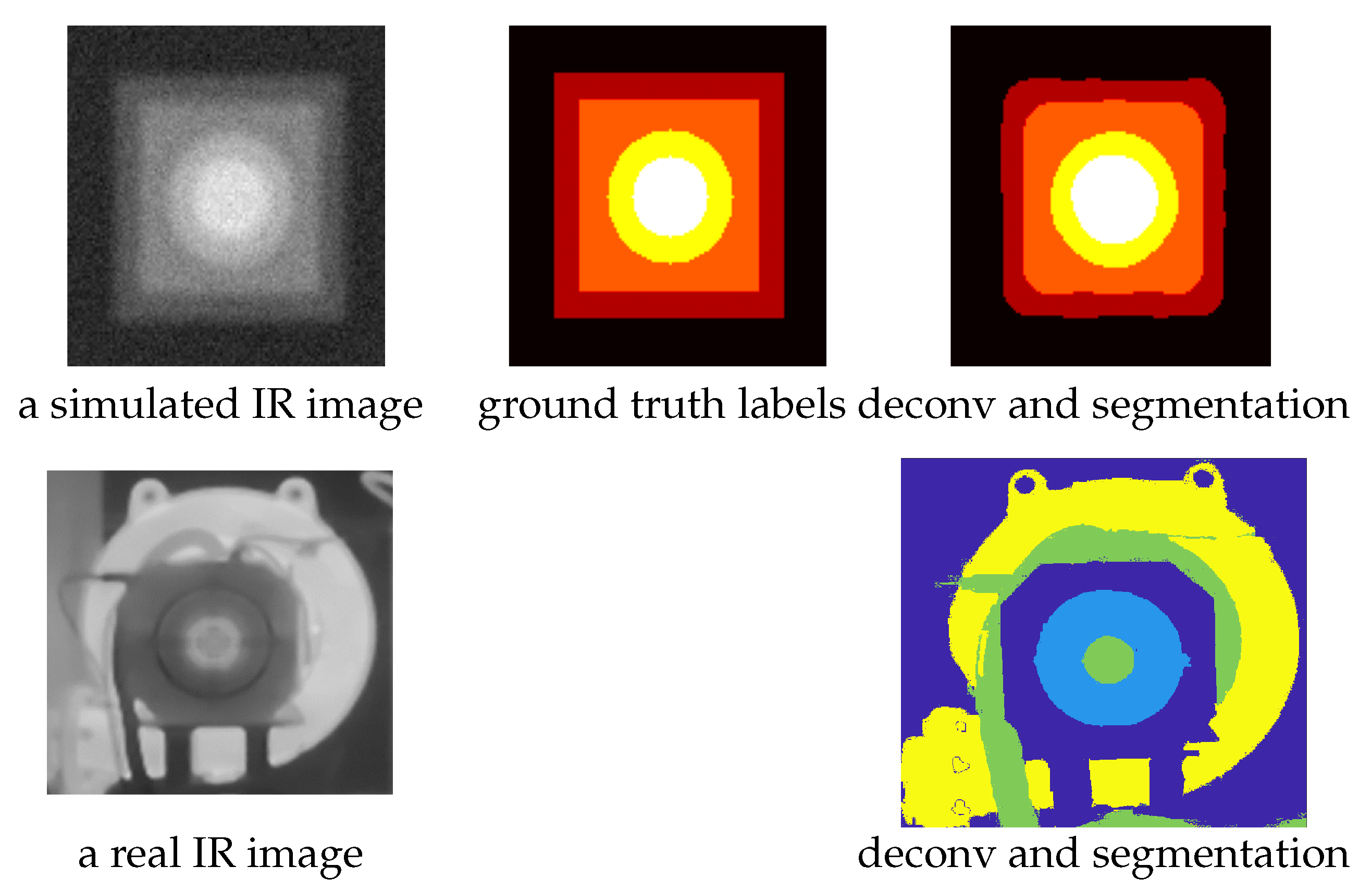
To train this NN, we can generate different known shaped images to consider as the ground truth and simulate the blurring effects of temperature diffusions via the convolution of different appropriate PSFs. We can also add some noise to generate realistic images. We can also use black body thermal sources and acquire different images at different conditions. All these images can be used for the training of the network. See an example of the obtained result in
Figure 9.
Author Contributions
Conceptualization and methodology, A.M.-D., N.C., L.W. and L.Y.; software, A.M.-D.; validation, A.M.-D., N.C., L.W. and L.Y.; formal analysis, A.M.-D.; investigation, resources, and data curation, N.C.; writing—original draft preparation, writing—review and editing, visualization and supervision, A.M.-D.; project administration and funding acquisition, N.C. and A.M.-D. All authors have read and agreed to the published version of the manuscript.
Funding
This research received no external funding.
Institutional Review Board Statement
Not applicable.
Informed Consent Statement
Not applicable.
Data Availability Statement
Data sharing is not applicable to this article.
Conflicts of Interest
The authors Ali Mohammad-Djafari and Ning Chu are the scientific researchers of Zhejiang Shangfeng Special Blower Company. The authors declare no conflict of interest.
References
- Ayasso, H.; Mohammad-Djafari, A. Joint NDT Image Restoration and Segmentation Using Gauss-Markov-Potts Prior Models and Variational Bayesian Computation. IEEE Trans. Image Process. 2010, 19, 2265–2277. [Google Scholar] [CrossRef] [PubMed]
- Tang, J.; Egiazarian, K.; Golbabaee, M.; Davies, M. The Practicality of Stochastic Optimization in Imaging Inverse Problems. IEEE Trans. Comput. Imaging 2020, 6, 1471–1485. [Google Scholar] [CrossRef]
- Zhu, Y.; Zabaras, N. Bayesian deep convolutional encoder–decoder networks for surrogate modeling and uncertainty quantification. J. Comput. Phys. 2018, 366, 415–447. [Google Scholar] [CrossRef]
- McCann, M.T.; Jin, K.H.; Unser, M. A Review of Convolutional Neural Networks for Inverse Problems in Imaging. Image Video Process. 2017, 34, 85–95. [Google Scholar] [CrossRef]
- Fang, Z. A High-Efficient Hybrid Physics-Informed Neural Networks Based on Convolutional Neural Network. IEEE Trans. Neural Netw. Learn. Syst. 2021, 33, 5514–5526. [Google Scholar] [CrossRef] [PubMed]
- Gilton, D.; Ongie, G.; Willett, R. Neumann Networks for Linear Inverse Problems in Imaging. IEEE Trans. Comput. Imaging 2020, 6, 328–343. [Google Scholar] [CrossRef]
- Gong, D.; Zhang, Z.; Shi, Q.; van den Hengel, A.; Shen, C.; Zhang, Y. Learning Deep Gradient Descent Optimization for Image Deconvolution. IEEE Trans. Neural Netw. Learn. Syst. 2020, 31, 5468–5482. [Google Scholar] [CrossRef] [PubMed]
- De Haan, K.; Rivenson, Y.; Wu, Y.; Ozcan, A. Deep-Learning-Based Image Reconstruction and Enhancement in Optical Microscopy. Proc. IEEE 2020, 108, 30–50. [Google Scholar] [CrossRef]
- Aggarwal, H.K.; Mani, M.P.; Jacob, M. MoDL: Model-Based Deep Learning Architecture for Inverse Problems. IEEE Trans. Med. Imaging 2019, 38, 394–405. [Google Scholar] [CrossRef] [PubMed]
- Chen, Y.; Lu, L.; Karniadakis, G.E.; Negro, L.D. Physics-informed neural networks for inverse problems in nano-optics and metamaterials. Opt. Express 2020, 28, 11618–11633. [Google Scholar] [CrossRef] [PubMed]
- Raissi, M.; Perdikaris, P.; Karniadakis, G.E. Physics-informed neural networks: A deep learning framework for solving forward and inverse problems involving nonlinear partial differential equations. J. Comput. Phys. 2019, 378, 686–707. [Google Scholar] [CrossRef]
- Mohammad-Djafari, A. Hierarchical Markov modeling for fusion of X-ray radiographic data and anatomical data in computed tomography. In Proceedings of the IEEE International Symposium on Biomedical Imaging, Washington, DC, USA, 7–10 July 2002; pp. 401–404. [Google Scholar] [CrossRef]
- Mohammad-djafari, A. Regularization, Bayesian Inference and Machine Learning methods for Inverse Problems. Entropy 2021, 23, 1673. [Google Scholar] [CrossRef] [PubMed]
- Giordano, R.; Broderick, T.; Jordan, M. Linear response methods for accurate covariance estimates from mean field variational Bayes. In Proceedings of the Advances in Neural Information Processing Systems, Montreal, QC, Canada, 7–12 December 2015. [Google Scholar]
- Chun, I.Y.; Huang, Z.; Lim, H.; Fessler, J. Momentum-Net: Fast and convergent iterative neural network for inverse problems. IEEE Trans. Pattern Anal. Mach. Intell. 2020, 45, 4915–4931. [Google Scholar] [CrossRef] [PubMed]
- Lucas, A.; Iliadis, M.; Molina, R.; Katsaggelos, A.K. Using Deep Neural Networks for Inverse Problems in Imaging: Beyond Analytical Methods. IEEE Signal Process. Mag. 2018, 35, 20–36. [Google Scholar] [CrossRef]
- Chang, J.H.R.; Li, C.L.; Poczos, B.; Kumar, B.V.K.V.; Sankaranarayanan, A.C. One Network to Solve Them All—Solving Linear Inverse Problems using Deep Projection Models. In Proceedings of the IEEE International Conference on Computer Vision 2017, Venice, Italy, 22–29 October 2017. [Google Scholar]
- Liang, D.; Cheng, J.; Ke, Z.; Ying, L. Deep Magnetic Resonance Image Reconstruction: Inverse Problems Meet Neural Networks. IEEE Signal Process. Mag. 2020, 37, 141–151. [Google Scholar] [CrossRef] [PubMed]
Figure 1.
General exponential family, with original parameters , natural parameters , expectations parameters , and their relations via the Legendre Transform.
Figure 1.
General exponential family, with original parameters , natural parameters , expectations parameters , and their relations via the Legendre Transform.
Figure 2.
Three linear NN structures, which are derived directly from quadratic regularization inversion method. The right part of this figure is adapted from [
16].
Figure 2.
Three linear NN structures, which are derived directly from quadratic regularization inversion method. The right part of this figure is adapted from [
16].
Figure 3.
A K layers DL NN equivalent to K iterations of the basic optimization algorithm.
Figure 3.
A K layers DL NN equivalent to K iterations of the basic optimization algorithm.
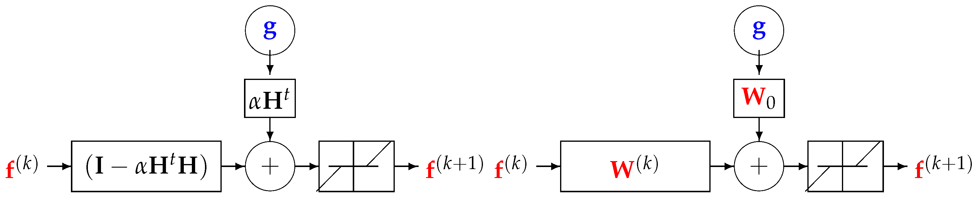
Figure 4.
A K layers DL NN equivalent to K iterations of a basic gradient-based optimization algorithm. A quadratic regularization results in a linear NN, while a regularization results in a classical NN with a nonlinear activation function. Left: supervised case. Right: unsupervised case. In both cases, all the K layers have the same structure.
Figure 5.
All the K layers of DL NN equivalent to K iterations of an iterative gradient-based optimization algorithm. The simplest solution is to choose and , . A more robust, but more costly approach, is to learn all the layers for , .
Figure 5.
All the K layers of DL NN equivalent to K iterations of an iterative gradient-based optimization algorithm. The simplest solution is to choose and , . A more robust, but more costly approach, is to learn all the layers for , .
Figure 6.
Training (top) and testing (bottom) steps in the first use of physics-based ML approach.
Figure 6.
Training (top) and testing (bottom) steps in the first use of physics-based ML approach.
Figure 7.
The proposed four groups of layers of NN for denoising, deconvolution, and segmentation of IR images.
Figure 7.
The proposed four groups of layers of NN for denoising, deconvolution, and segmentation of IR images.
Figure 8.
Example of expected results in deterministic methods. First row: a simulated IR image (left), its ground truth labels (middle), and the result of the deconvolution and segmentation (right). Second row: a real IR image (left) and the result of its deconvolution and segmentation (right).
Figure 8.
Example of expected results in deterministic methods. First row: a simulated IR image (left), its ground truth labels (middle), and the result of the deconvolution and segmentation (right). Second row: a real IR image (left) and the result of its deconvolution and segmentation (right).
Figure 9.
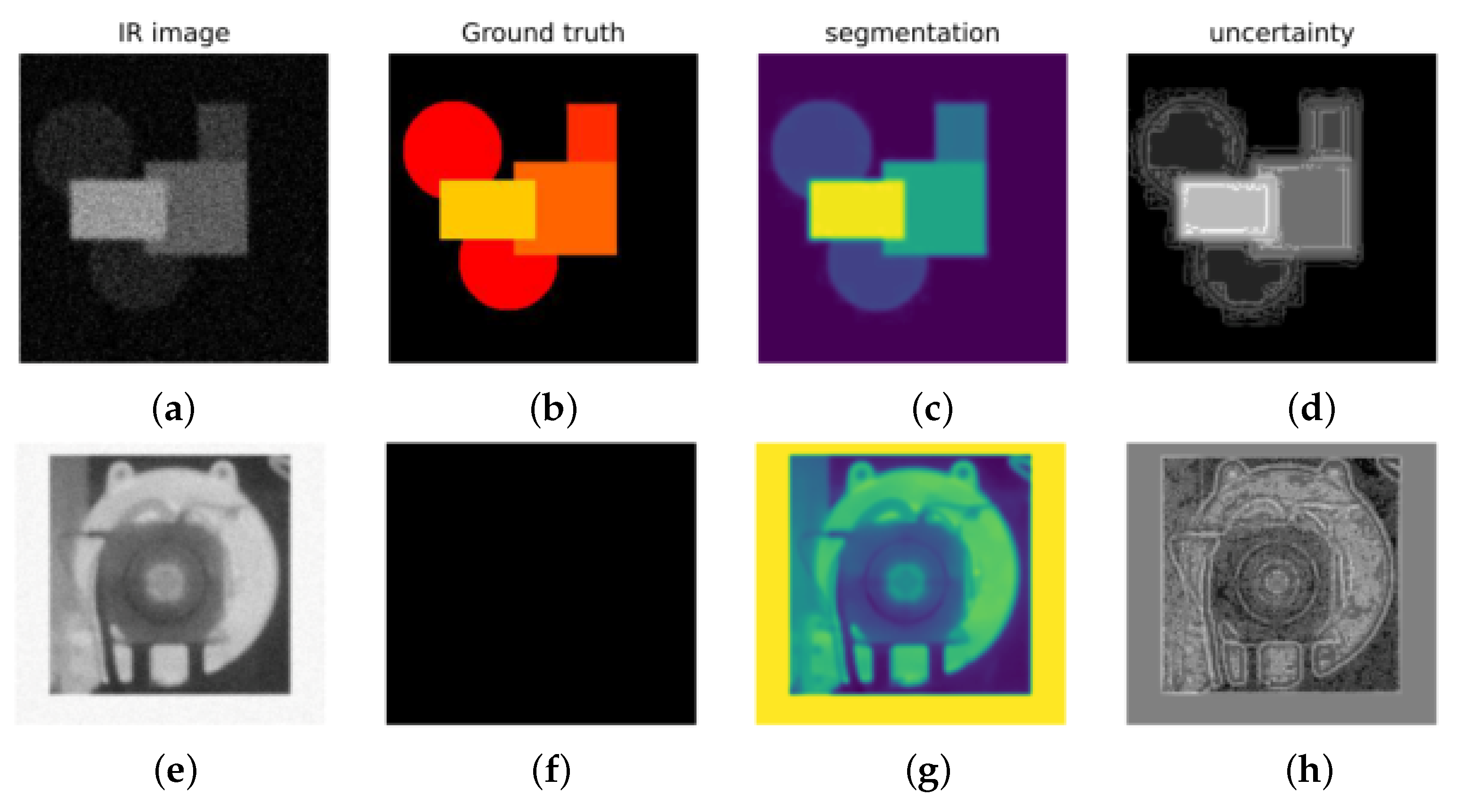
Example of expected results in Bayesian methods. First row from left: (a) simulated IR image, (b) its ground truth labels, (c) the result of the deconvolution and segmentation, and (d) uncertainties. Second row: (e) a real IR image, (f) no ground truth, (g) the result of its deconvolution and segmentation, and (h) uncertainties.
Figure 9.
Example of expected results in Bayesian methods. First row from left: (a) simulated IR image, (b) its ground truth labels, (c) the result of the deconvolution and segmentation, and (d) uncertainties. Second row: (e) a real IR image, (f) no ground truth, (g) the result of its deconvolution and segmentation, and (h) uncertainties.
| Disclaimer/Publisher’s Note: The statements, opinions and data contained in all publications are solely those of the individual author(s) and contributor(s) and not of MDPI and/or the editor(s). MDPI and/or the editor(s) disclaim responsibility for any injury to people or property resulting from any ideas, methods, instructions or products referred to in the content. |
© 2023 by the authors. Licensee MDPI, Basel, Switzerland. This article is an open access article distributed under the terms and conditions of the Creative Commons Attribution (CC BY) license (https://creativecommons.org/licenses/by/4.0/).


