Impact of Flexibility Implementation on the Control of a Solar District Heating System

Abstract

Renewable energy sources, distributed generation, multi-energy carriers, distributed storage, and low-temperature district heating systems, among others, are demanding a change in the way thermal networks are conceived, understood, and operated. Governments around the world are moving to increase the renewable share in energy distribution networks through legislation like the European Directive 2012/27 in Europe, and solar energy integration into district heating systems is arising as an interesting option to reduce operation costs and carbon footprint. This conveys an important investment that adds complexity to the management of thermal networks and often delays the return on investment due to the unpredictability of renewable energy sources, like solar radiation. To this end, this paper presents an optimisation methodology to aid in the operative control of an existing solar district heating system located in the northwest of France. The modelling of the system, which includes a large-scale solar field, a biomass boiler, a gas boiler, and thermal energy storage, was previously built in Dymola. The optimisation of this network was performed using MATLAB’s genetic algorithm (GA) and running the Dymola model as functional mock-up units, FMUs, using Simulink’s FMI Kit. The results show that the methodology presented here can reduce the current operation costs and improve the use of the daily storage of the DH system by a combination of mass flow control and the implementation of a flexibility function for the end-users. The cost-per-kWh was reduced by as much as 16% in a single day, and the share of heat supplied by the solar field on this day was increased by 5.22%.

1. Introduction

Today, district heating systems account for around 12% of the total heat demand in the building sector in Europe. In the case of France, the Heat Road Map for 2050 expects that DH will expand to provide at least 25% of domestic and commercial heat by the end of 2050, but this fraction was 7% in 2019 [1].

Thanks to DH’s ability to collect, store, and transport heat from industrial processes, waste management activities, and surplus electricity from renewable sources, it could become an important tool to offset the temporal and spatial mismatches that exist among the generation, supply, and demand of energy [2]. However, to propose these new services, outdated reference control strategies [3] have to be rethought, as illustrated by the numerous studies on optimal control strategy development [3,4,5,6,7].

By construction, DH optimisation results in a hard optimisation problem because of their MINLP formulation (mixed integer non-linear program). To avoid excessive computational times, one approach can consist of linearising the problem, as in [8], for example. The reported work presents a linearized control-oriented model of borehole thermal energy storage (BTES) with a weekly control time-step and a yearly horizon. The control tests the operating conditions of the storage system under two different electricity CO₂ intensity conditions: one constant during the year and another that is relaxed during the summer. Due to seasonal variations, having a higher heat pump efficiency in winter while accepting a lower one in summer helped the control achieve CO₂ emissions savings of 2.2% to 4.3%.

While linear programming can be employed for optimizing DH systems, the inherent non-linearity of heat networks makes non-linear approaches more attractive, as illustrated, for example, in [9]. A model-based predictive control strategy for the district heating system at the Drake Landing Solar Community in Okotoks, Canada has been proposed, aiming to optimize the temperature difference across solar collectors and the flow rate in the BTES loop to minimize pump electricity consumption while maintaining a solar fraction of 90%. The flow rate was optimised at constant values for 4 h over the next 48 h, with a control horizon of 12 h to account for day and night. Yearly evaluations demonstrated potential pump energy savings of 38% and a reduction in greenhouse gas emissions of up to 32%.

While various tools exist for solving non-linear optimisation problems, the literature indicates a preference for using metaheuristic algorithms, such as the genetic algorithm, as seen in [10,11]. The study in [12] introduced a method for optimizing DH networks with distributed generation plants. A genetic algorithm optimised the system dispatch by evaluating the network’s state based on temperatures and flows at generation plants, achieving simultaneous optimisation of all heat plants. The results indicate fuel and pumping cost savings. Wang et al. [13] proposed an optimisation model using a genetic algorithm to minimize power consumption in distribution pumps within a DH network, integrating renewable energy sources. The results highlight that slight changes in renewable heat source power can significantly impact pump power demand. Hirvonen et al. [14] presented a study optimizing a solar community in Finland, utilizing TRN-SYS© for simulation and a genetic algorithm for optimisation. The system comprised solar collectors, solar panels, centralized short-term storage, and borehole thermal storage, with the results showcasing the potential for up to 44% of heat demand from the storage system and an 80% reduction in electricity consumption compared to the base case.

As systems grow in complexity or when variables have conflicting effects on solutions, a multi-objective approach is often employed. In [15], the authors aimed to optimize supply capacities and the yearly operation of a DH network with thermal storage, considering total cost, carbon dioxide emissions, and exergy destruction minimization as objectives. The simulation model, written in Julia, used the Clp linear programming solver to obtain solutions. This study was later extended in [16] to propose an “exergy tax” alongside a carbon tax, effectively reducing natural gas consumption in heat-only boilers.

While historical optimisation efforts in DH have predominantly focused on technical and economic aspects, a notable shift involves actively incorporating end-users and the distribution network into optimisation routines and objectives. A key focus in DH optimisation is now on the concept of “flexibility,” defined as a DH network’s ability to shift its energy supply/demand in time or magnitude. This introduces the potential for demand response (DR) and network response strategies in addition to existing dispatch strategies [2], where various flexibility sources are explored, including the thermal inertia of buildings, network heat inertia, storage utilization, and smart thermal networks.

Illustrating the impact of heat inertia on supply flexibility, Wernstedt et al. [17] demonstrated the potential to curtail up to 10% of demand for short periods without consumer notice, reducing demand at substations by around 4%. In [18], a model predicted the power demand of commercial buildings and possible alterations to use them as short-term energy storage to balance grid power flows. Zhou et al. [19] investigated the effects of implementing DR and electrical energy storage on distribution systems, focusing on energy payback, flexibility, and storage efficiency. A recent study [20] explored the potential of DR on energy supply in buildings, accounting for heat inertia. The results indicate that leveraging building heat inertia as short-term storage enables DR events, where supply is completely curtailed, for over 1.5 h before occupants feel discomfort.

Based on this review of the literature, this paper aims to evaluate the use of a GA optimisation strategy based on mass flow control coupled to a flexibility function to reduce the cost function of a real DH network with solar generation and energy storage while potentially increasing its solar fraction. It focuses on the methodology presentation and on first results.

2. Methodology

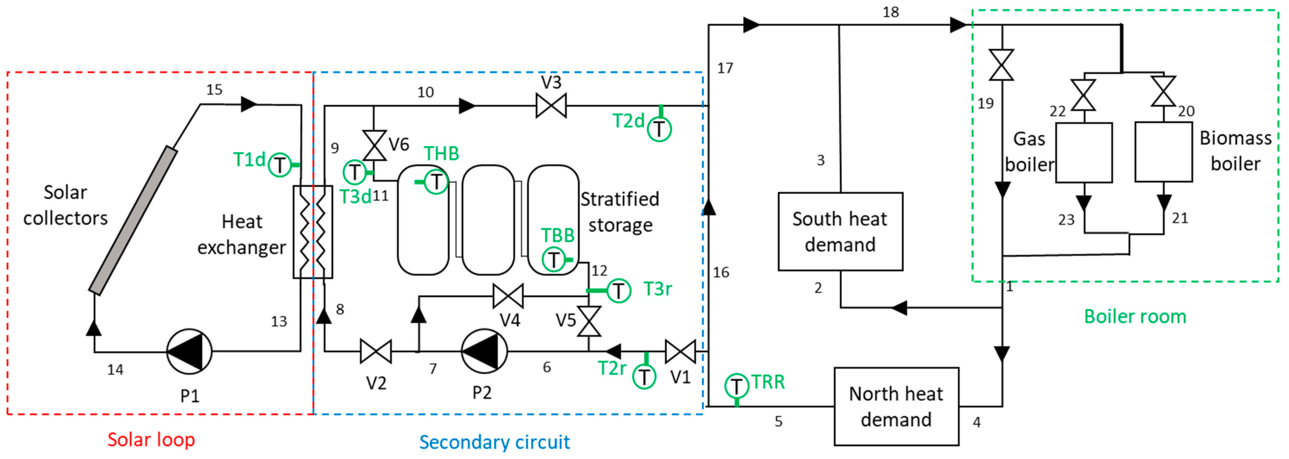
2.1. Case Description

The methodology described in this paper was applied to a simulation model built in Dymola [21] representing an existing solar district heating system in the Northwest of France, in the city of Chateaubriant. This model was developed in the frame of SunSTONE, a project that aims to develop a smart control tool for DH in a system with a high solar fraction DH and seasonal thermal storage [22]. To achieve this, a virtual twin of an existing DH system was built in Dymola, converted into a functional mock-up unit using Visual Basic, and run in a MATLAB optimisation through Simulink’s FMI Kit (Figure 1).

A simplified layout of the model created in Dymola, referred to here as the SunSTONE model, is shown in Figure 2. The DH network supplies two clusters of consumers around 2.5 km away through two branches (North and South). The total annual heat demand of the system is of 18.6 GWh, which supplies heat for domestic and commercial space heating and hot water. The returning flows from the two branches are mixed before entering the boiler room, composed of a gas boiler and a biomass boiler. A solar thermal field on the North branch is used to preheat the returning flow before it is mixed with the return flow from the South branch. The solar field is composed of 200 flat-plate collectors with an inclination of 30°. One hundred and forty-six of these panels face south and 54 face 7° southeast. A secondary loop containing three tanks for short-term thermal storage (STTS) is connected to the solar field through a heat exchanger. The main characteristics are summarised in

Table 1. Technical data of the main Chateaubriant components.

Component	Nominal Capacity/Size
Gas boiler	6 MWth
Biomass boiler	3 MWth/0.75 MWth (min.)
Heat pump	40 kWel
Solar field	1.7 MWth peak (2340 m2)
STTS	150 m3

; for a full description of the SunSTONE model, see [23].

The operation costs were dynamically evaluated using the Dymola tool (the energy, exergy, and cost balances are detailed in [23]) based on exergo-economic analysis conducted according to the specific exergy costing (SPECO) method [24]. In this manner, the optimised costs did not solely stem from decreased fuel usage; rather, they resulted from comprehensive alterations to the exergy streams within the system, encompassing the annualized capital cost of the component. This calculation takes into account the component’s lifespan and the prevailing interest rate. These costs are consolidated into a singular metric referred to as the cost per kilowatt-hour (kWh) of the system. This metric was computed for each operational period, equivalent to every 20 min. The main economic assumptions are summarised in

Table 2. Economic data.

Parameter	Value
Cost of electricity [EUR/kWh]	0.14
Cost of gas [EUR/kWh]	0.039
Cost of biomass [EUR/kWh]	0.023
Gas boiler investment cost [Mio EUR]	1.20
Biomass boiler investment cost [Mio EUR]	2.10
Solar collector field investment cost [Mio EUR]	1.35
Lifetime of all components except gas boiler [year]	20
Gas boiler lifetime [year]	25
Interest rate [%]	3.75

.

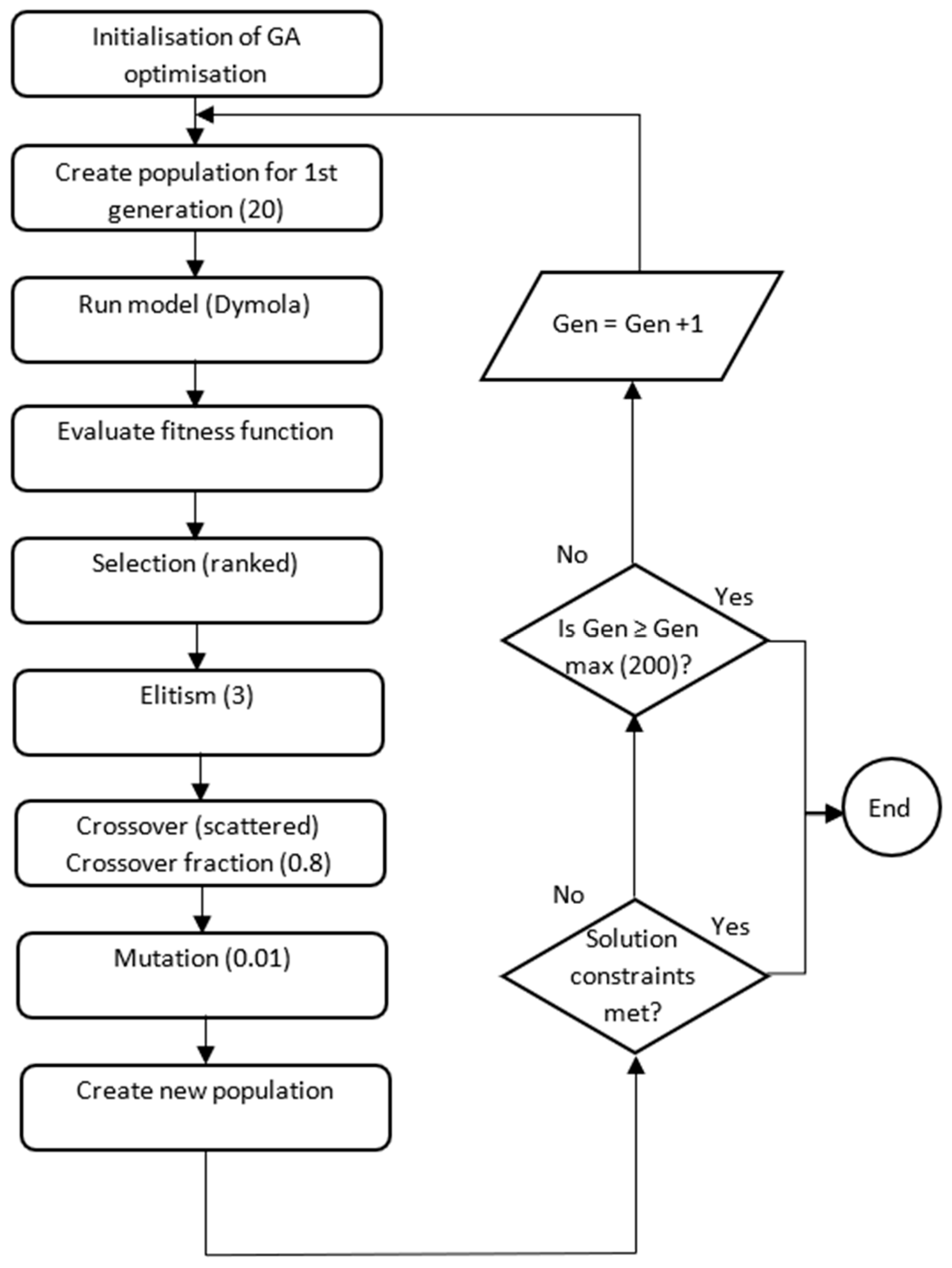
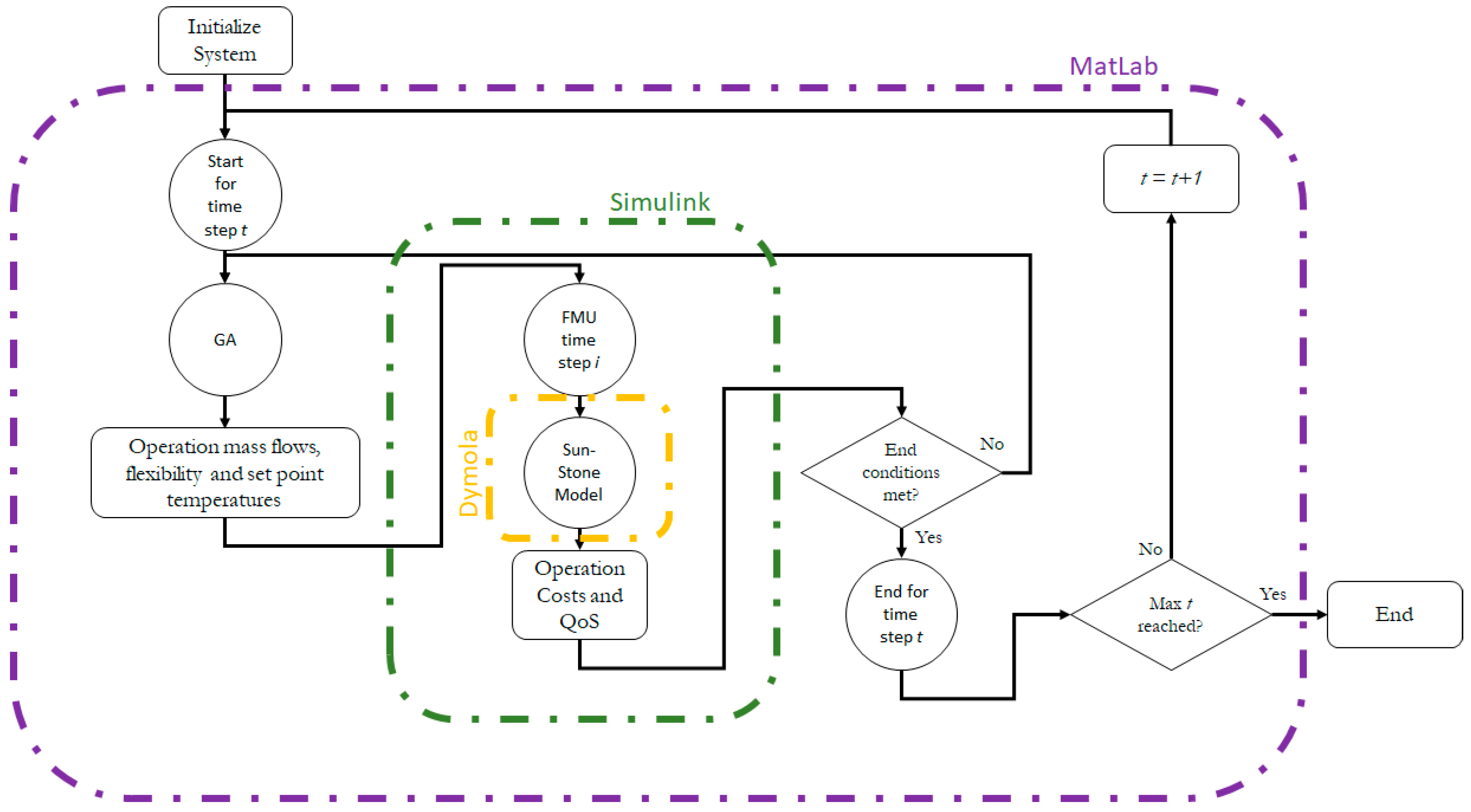
2.2. Optimisation Problem Solving Strategy

The proposed optimisation aims to reduce the cost per kWh associated with the day-to-day operation of the network described above. To achieve this, it was necessary to find the heat flows in the network (temperature and mass flow rate) that would allow the supply to reach the consumers without compromising the quality of service (QoS) while minimising the overproduction of heat and using the available storage. An example of such an approach for the optimisation of DH networks can be found in [25].

GA is an optimisation algorithm based on metaheuristics, which are popular optimisation techniques widely regarded as being efficient approaches for hard optimisation problems [26]. Hence, it has been extensively used to optimise district heating systems, which fall in this category of hard problem because of the non-linearities and the mix of integer and continuous variables obtained by default in their formulation (see, for example, [27] or [9]). GA is inspired by the natural evolution of populations as seen in the wild [28]. It can arrive at near-optimum solutions in cases where non-continuous variables are present so that no deterministic mathematical modelling is possible without having to adapt deeply to each problem, as well as cases when the model is better approached as a black box. GA is able to explore a large space without becoming stuck in local maximum or minimum solutions when properly constructed [29].

Typically, GA consists of a set of variables, a fitness function, and a set of constraints. In a GA optimisation process, the variables (called chromosomes) are arranged into a chain and fed into the fitness function to give a solution. If the chromosomes, the solution, and any mid-steps are all within the constraints, the solution is considered feasible and stored, otherwise it is discarded. Each feasible solution is called an individual, with a combination of individuals being called a population. The population size is usually set to a specific desired value and solutions are searched until the number of individuals matches the population [30].

To find the optimum value of the fitness function, several populations must be analysed, each of them being called a generation. Every new generation relates to the previous one by the processes of selection, elitism, crossover, and mutation [30]:

• Selection: the individuals of a population are sorted according to the value of the fitness function and chosen or not for crossover (akin to natural selection).
• Elitism: the higher-ranked individuals are passed on to the next generation with no change (akin to cloning).
• Crossover: two individuals are chosen as parents and their chromosomes are combined to create new “child” individuals that, if they are a feasible solution, pass to the new generation (akin to sexual reproduction).
• Mutation: single chromosomes of an individual have a chance to acquire a new value; if feasible, the child solution passes on to the next generation (similar to a natural mutation).

In our case, the size of the population was set to 20, the maximum number of generations to 200, the crossover scheme was to be scattered with a crossover fraction of 0.8, the mutation chance was set to 0.01, and the elite count was set to 3. The individuals were composed of 36 chromosomes in sets of 4. Each set corresponded to 20 min of operation, the chromosomes in a set including the mass flow rates on each branch (North and South), and the flexibility function of each substation associated to a cluster of consumers (North and South). The nine 20 min sets therefore correspond to an optimisation horizon of three hours. The diagram of an individual chromosome can be seen in Figure 3; the diagram of the GA optimisation can be seen in Figure 4.

While the GA explores different mass flow rates, the supply temperature of the DHN is calculated inside the SunSTONE model as a function of the ambient temperature. By varying the mass flows, each proposed operation by the GA gives different return temperatures that could go directly into the generation loop, into the solar loop, or into the storage loop. The fitness function evaluates the variables to find the best combination that supply the demand at the lowest operating cost (Equation (1)).

$$MIN:f\left({Cost}^t\right)={\sum }_{i=0}^t\left({kWh}_{Gen}^i\times C^i\right)+g\left({kWh}_{gen}^t\right)$$

(1)

where ${kWh}_{Gen}^i={kWh}_{sol}^i+{kWh}_{bio}^i+{kWh}_{gaz}^i$.

In Equation (1), $t$ is the optimisation period, $i$ the intra-optimisation time step, ${Cost}^t$ the total cost of operation for the evaluated period, ${kWh}_{Gen}^i$ the total generation, ${kWh}_{sol}^i$ the heat generation from the solar field, ${kWh}_{bio}^i$ the heat generation from the biomass boiler, ${kWh}_{gaz}^i$ the heat generation from the gas plant, and $C^i$ the total cost over the time step.

A penalty function $g\left({kWh}_{gen}^t\right)$ affects the fitness function when the quality of service (QoS) is compromised or when energy is being wasted (Equation (2)).

$$g\left({kWh}_{gen}^t\right)={SnD}^t\times {\overline{C}}^t\times exp\left(\frac{{SnD}^t}{Q_D^t}\right)$$

(2)

In this equation, ${kWh}_{gen}^t$ is the total energy generated in period $t$, $SnD$ represents the deficit (demand not supplied) or the surplus (overgeneration), ${\overline{C}}^t$ the average cost per kWh, and $Q_D^t$ the total demand for the period. As in [25], the exponential increases the value of the penalty function more and more as the deficit or surplus increases.

The GA optimisation also includes a flexibility function as a variable. Flexibility functions can be as simple or as complex as desired. For this methodology, which does not focus on the development of flexibility functions, the function was defined as the proportion of the heat supply that can be interrupted without adversely affecting the QoS of the end-users when network rebalancing is required or the network is at risk of losing its QoS (i.e., the simulation shows very high deficits over a given period). Flexibility is encoded in chromosomes by an integer value between “1” and “5”. A value of “1” indicates that all the demand is supplied to the branch, “2” that there is a 0.5% reduction in the supply, and every unit after indicates a further 0.5% supply curtailment to a maximum of 2% when the function reaches a value of “5”. A constraint function was added to guarantee that no consecutive 20 min periods have a flexibility function coefficient greater than “1”. These coefficients are shown in blue in Figure 3.

With the optimisation algorithm and fitness function defined above, the SunSTONE model was optimised as shown in Figure 5. The GA was started with an initial population formed of seven seeded individuals and thirteen random ones. The variables were the mass flows and the value of the flexibility function. The variables were used to simulate the next 3 h in 20 min intervals.

The SunSTONE model was run for every individual and the GA operated as described in Figure 5. When an optimum solution is found, the first 12 chromosomes of the fittest individual were saved as the solution for the first hour, and the optimisation advanced by 1 h. In this way, each hour was optimised three times: once with the two previous hours, once with the previous hour and the following, and once with the following two hours. The 24 remaining chromosomes were used to create four of the seven seed individuals for the next optimisation period (the remaining three are the lower bound, the upper bound, and the measured values obtained as part of the SunSTONE project). The 3 h period (namely the optimisation horizon), which advanced by 1 h for every successful optimisation (the optimisation sliding window), ensured that local solutions did not adversely affect the solution of subsequent time periods. A comparison of the effects of single versus sliding window optimisation can be found in [25].

The optimisation took between 10 and 25 min to optimise each hour of operation. Due to the use of a horizon, information on future demands and weather conditions was required for each optimisation cycle. In the methodology presented, all optimisations were performed using data measured at the site during a previous year. For real-life implementation, this information can come from a predictive model or from historical and environmental data that update the information every time the optimisation window moves to the next hour. In this way, the optimisation continues until the entire designated period is evaluated, i.e., a day, a week, or even a year, and the individual results can be used for daily control.

3. Results and Discussion

February 14 with data from 2019 was chosen for the present study (characteristics in Figure 6). Since it was a winter day with good solar irradiation, a significant fraction of the supply could be provided by the solar collectors and the daily heat storage tank.

Figure 7 shows the cost per kWh generated for each case. The average cost for the reference case is barely above 0.050 EUR/kWh, while for the optimisation solution it is of 0.047 EUR/kWh. The main difference between them is the spread of the costs, as 50% of the costs from the reference case are between 0.044 EUR/kWh and 0.086 EUR/kWh, with the min-max being at 0.037 EUR/kWh and 0.105 EUR/kWh, respectively. For the optimised case, 50% of the costs are between 0.033 EUR/kWh and 0.064 EUR/kWh, with the min-max being at 0.018 EUR/kWh and 0.098 EUR/kWh. Some values can be found out of this range, but they are few in number and do not affect the overall results.

To understand the reduction in specific costs achieved, the duration curves of the system are shown in Figure 8. The optimisation case has similar generation to the reference case but it is distributed differently among the three heat sources (biomass boiler, gas boiler and solar field). In the optimisation, the biomass boiler’s use is reduced by 1.5% while the use of the gas boiler is increased by 28.23%. In the optimisation, the solar field also yields 5.22% more heat than in the reference case.

Figure 9 shows that the optimisation has a wider range of mass flows during this day’s operation than the reference case. The average mass flows for the reference case are of 26 kg/s in the North Branch and of 21 kg/s in the South Branch compared to 35 kg/s and 37 kg/s, respectively, for the optimisation case. The main difference between the two cases comes from the range of mass flows in which each of them works: while all flows in the reference case remain between 7 kg/s and 30 kg/s, those for the optimisation range from 9 kg/s to 54 kg/s with flows distributed in this range.

In order to assess the sensitivity to constraints in flow variation, three distinct cases were tested: no constraints for the change in mass flow between time steps (yellow), hard constraint of ±30 kg/s between time steps (green), and what we call a soft constraint of the change between time steps (blue) and the results reported in Figure 10. In this case, the constraint of ±30 kg/s was maintained if, and only if, the solution for the studied window was better than for the reference case. Otherwise, it was allowed to search for the best change in mass flow unconstrained. When unconstrained, the model gave a solution that was better than the reference case but required the system to change mass flows rapidly and steeply. These changes are unrealistic for the system and thus the solution is not viable. With the hard constraint (no change greater than 30 kg/s between time steps), the obtained solution exhibits little variation between time steps and is viable, but is worse than the reference case in terms of performance. The soft constraint results in greater variation in mass flows, but maintains the change in mass flow below 6 kg/s in most time steps, which is viable. The soft constraint was kept for the rest of the study.

The average return temperature distributions were plotted in Figure 11 for the reference and the optimised cases. Comparing the average values, the optimisation resulted in a significant increase for both branches (South Branch: 76 °C for the reference vs. 82 °C for the optimisation; North Branch: 81 °C for the reference vs. 89 °C for the optimisation). This trend is a direct consequence of the change in control strategy, which allows overproduction to a certain extent, resulting in an increase in the temperature of the distribution network.

To add information to the temperature distribution, the state of the storage is presented (Figure 12). The storage was depleted in the morning and began charging at midday in both cases. In the reference case, charging continued for almost five hours, after which the storage was rapidly discharged to meet demand. After this initial discharge, the storage went through a period of alternating charge and discharge phases. This behaviour can be explained by the fact that the reference case generally overproduces during peak hours and then stores the heat that is not consumed. This mode of operation contrasts with the optimisation case, where storage management changes. Instead of having a period of charging during the midday hours followed by discharging, optimisation makes more dynamic use of the stored energy to reduce the use of fuels during this period. This reduces not only the amount of energy stored, but also the costs. Because the optimisation also reduces overproduction by guaranteeing supply through control, there is less excess heat sent to the storage tanks after hours of sunshine.

Finally, Figure 13 presents the results of the flexibility function. Each bar indicates an instance on which supply in a specific branch is reduced by the amount indicated by the height of the bar. Both branches used flexibility a similar number of times, 16 times for the North Branch, 18 times for the South. The extent of the flexibility in the North Branch remained below 1% during most of its occurrences, while the South Branch required flexibilities higher than 1.5% for half of its occurrences. These results show that the network studied does benefit from flexibility, but not to the same extent as other networks (see [25]), where flexibility can be used all the time.

The combination of all these results describes how controlling the mass flow rates and implementing a flexibility function can be used to lower the operation costs over a selected period (not necessarily a single day) in combination with modelling and optimisation:

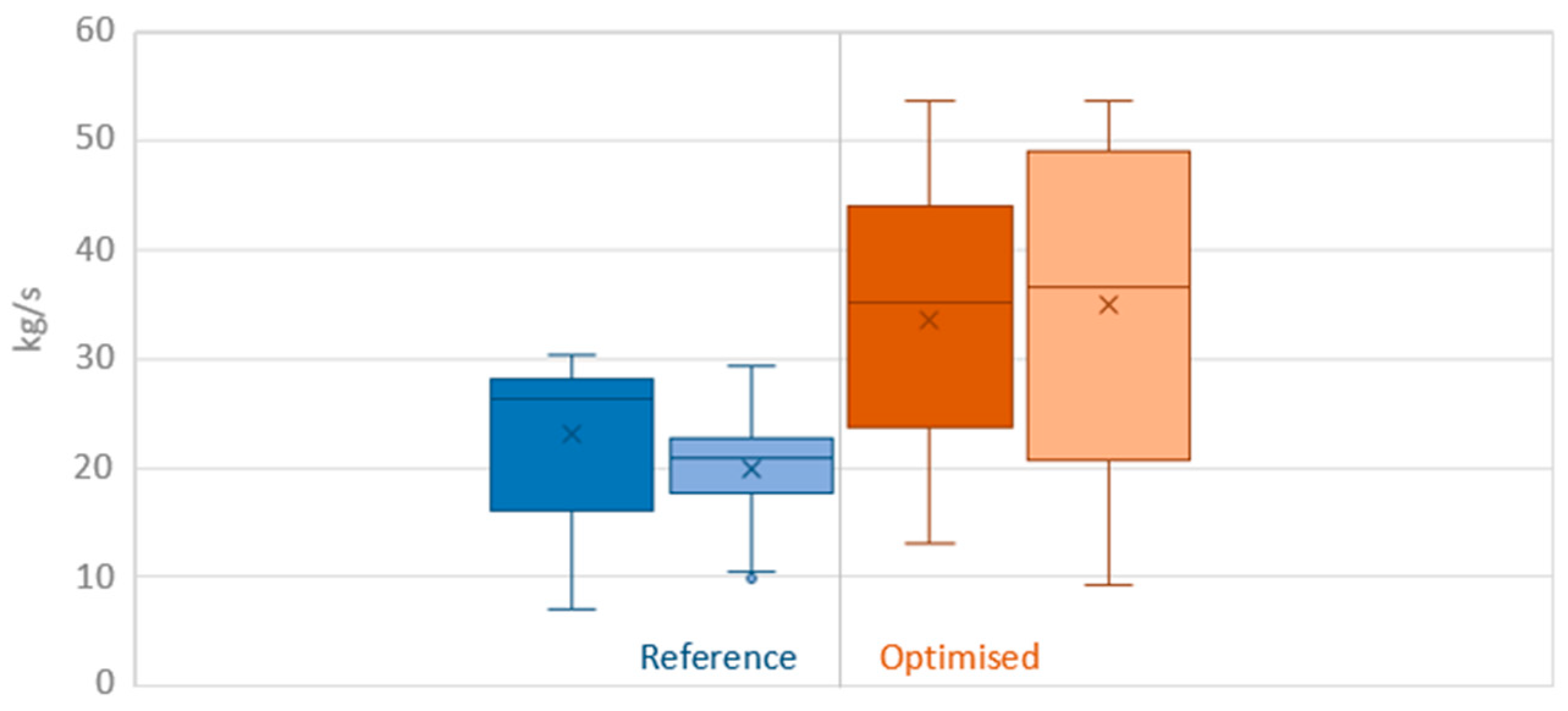
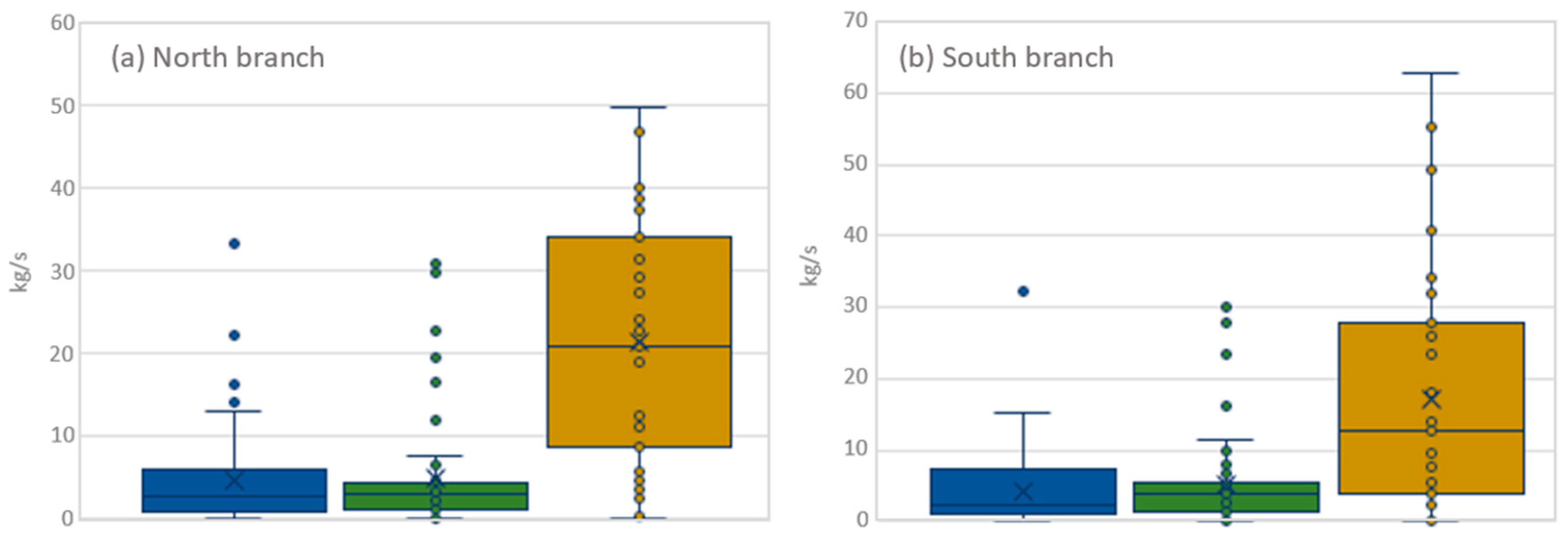
• Having a model capable of predicting how changes in the operation of a network affect its behaviour, combined with optimisation enabling the benefits of heat network inertia to be exploited. The ability to vary the mass flows ensures that energy already in the system is not wasted and that supply arrives on time. This is performed in a number of ways. When there is surplus energy in the system, mass flows can be reduced, thus lowering the return temperature. When demand is expected to go up, mass flows can be increased to raise the supply temperature of the network in anticipation. When demand goes up before the network is ready to meet it, mass flows can be increased to reduce the time during which end users risk a loss of QoS.
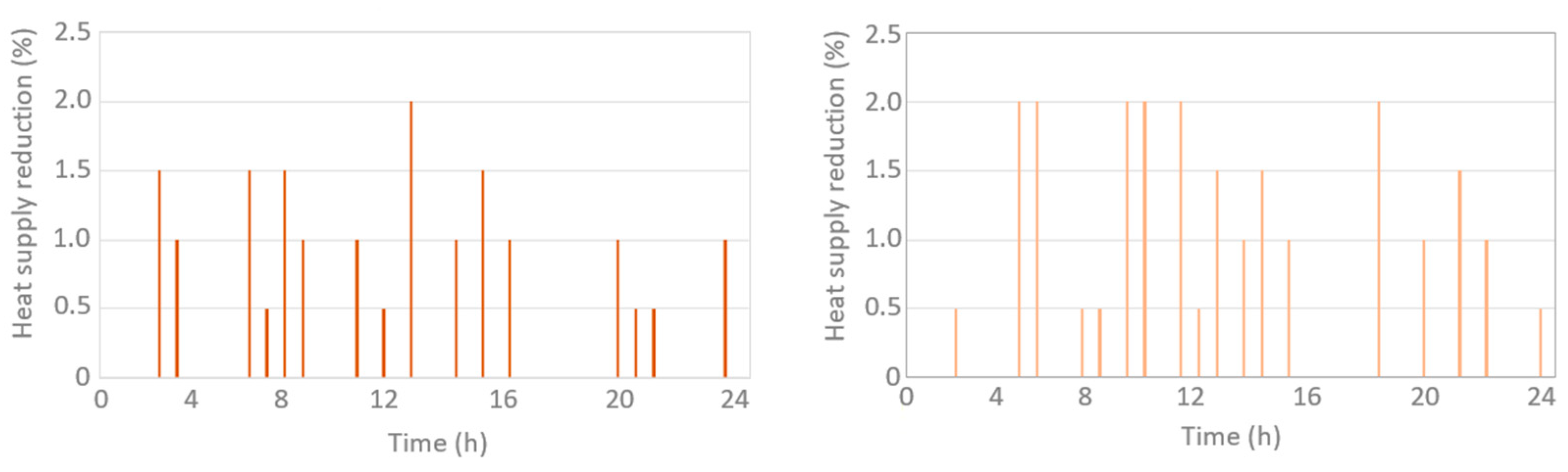
• The inertia of the network alone might not be sufficient to play the role of buffer whenever steep changes in supply or demand occur. While it can be harnessed to reduce costs, when sudden or major imbalances occur, it is also feasible to exploit the flexibility of the end users. Buildings do not immediately lose their comfort zone when heat is interrupted (unlike electricity, where any curtailment is immediately felt), allowing a small window in which supply can be reduced or completely cut out without the consumer noticing. This window varies from end user to end user, but a general flexibility function can be used to help the demand to rebalance the network and to prevent any major losses in the QoS. The use of a flexibility function is cheaper than reactive generation, aiding also in reducing costs.
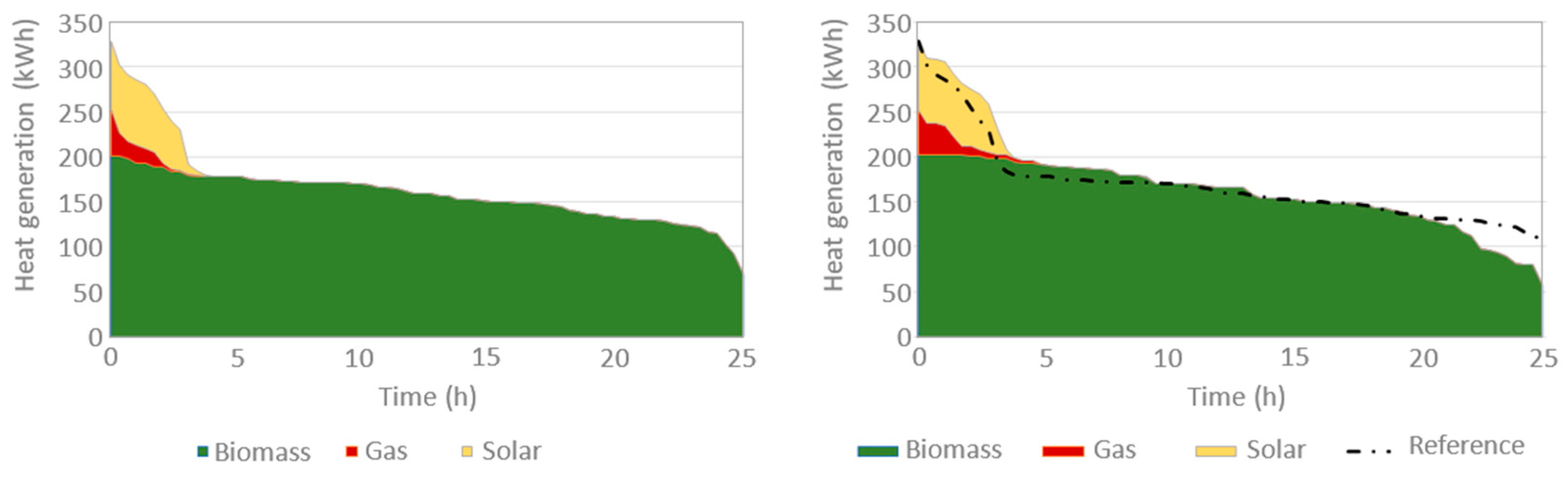
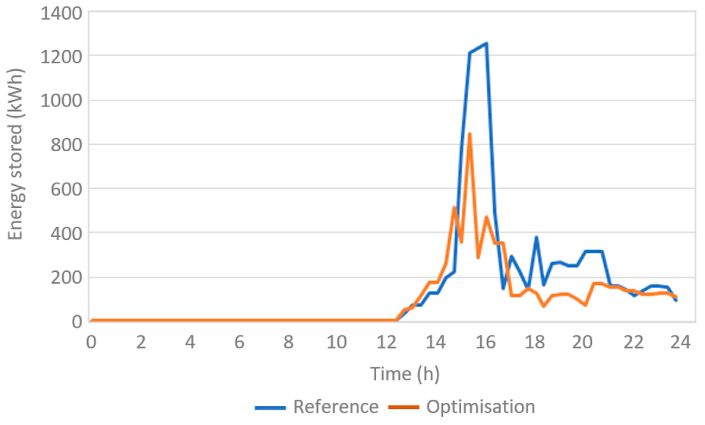
• A second use of the model in combination with optimisation, regardless of having a flexibility function or not, is a different management of existing storage. Instead of using storage for excess energy during sunny hours and overproduction during evening hours, optimisation proposes using it more dynamically to avoid or reduce the use of fuels in the boiler room. In this way, even if the storage does not reach its maximum load, costs will still be reduced, and the solar fraction of the system met.

All these effects combined explain how optimisation achieves reduction in operation costs while maintaining, and even increasing at times, the QoS.

4. Conclusions

This article aims to assess the impact of an optimal control on solar district heating (SDH) networks’ performance. A penalty function was introduced to reduce the heat supplied to a consumer substation when an event could lead to a significant increase in network costs if the entire supply had to be guaranteed. To achieve this, the proposed methodology uses a SDH model developed by INSA via Dymola in combination with a GA optimisation based on mass flow control, aiming at reducing the specific cost of heat (EUR/kWh).

The solution resulting from GA optimisation has a specific cost 16.03% lower on average, and an increase in heat supplied from the solar field of 5.22%.

In addition, after properly defining the constraints for the mass flow rates, the solution has a wider range of mass flow rates and higher return temperatures than the reference case. The total generation is similar to that of the reference case, but higher use of the gas plant and longer duration curves at high capacities were obtained.

As for the penalty function, 34 instances of flexibility exist in the optimisation solution for the day studied, with the South Branch having 18 and the North Branch 16. The characteristics of the network, in particular the existence of storage, limit the use of the flexibility, but it nevertheless has positive effects on network management and cost reduction. Indeed, from these first results, it appears that including a “quality of service“ approach for the optimisation of the control of a solar district heating network can lead to significant cost savings (i.e., 6% in the present case) and result in new strategies for short-term storage.

Lastly, this optimisation, while complex and mathematically intensive, was able to produce results for a whole hour of operation in less than 25 min, making it a viable option for daily control but not necessarily for real-time control.

As a perspective, work is currently under progress to extend the application of the proposed methodology to more complete cases (incl. considered time period). To tackle the computing time issue, surrogate modelling will be explored as well [31].

References

1. Connolly, D.; Lund, H.; Mathiesen, B.V.; Werner, S.; Möller, B.; Persson, U.; Boermans, T.; Trier, D.; Østergaard, P.A.; Nielsen, S. Heat Roadmap Europe: Combining District Heating with Heat Savings to Decarbonise the EU Energy System. Energy Policy 2014, 65, 475–489. [Google Scholar] [CrossRef]
2. Schrammel, H.; Kelz, J.; Gruber-Glatzl, W.; Halmdienst, C.; Schröttner, J.; Leusbrock, I. Increasing Flexibility towards a Virtual District Heating Network. Energy Rep. 2021, 7, 517–525. [Google Scholar] [CrossRef]
3. Mazhar, A.R.; Liu, S.; Shukla, A. A State of Art Review on the District Heating Systems. Renew. Sustain. Energy Rev. 2018, 96, 420–439. [Google Scholar] [CrossRef]
4. Bouhafs, F.; Mackay, M.; Merabti, M. Links to the Future: Communication Requirements and Challenges in the Smart Grid. IEEE Power Energy Mag. 2012, 10, 24–32. [Google Scholar] [CrossRef]
5. Vesterlund, M.; Toffolo, A.; Dahl, J. Optimization of Multi-Source Complex District Heating Network, a Case Study. Energy 2017, 126, 53–63. [Google Scholar] [CrossRef]
6. Zheng, J.; Zhou, Z.; Zhao, J.; Wang, J. Function Method for Dynamic Temperature Simulation of District Heating Network. Appl. Therm. Eng. 2017, 123, 682–688. [Google Scholar] [CrossRef]
7. Vandermeulen, A.; van der Heijde, B.; Helsen, L. Controlling District Heating and Cooling Networks to Unlock Flexibility: A Review. Energy 2018, 151, 103–115. [Google Scholar] [CrossRef]
8. Fiorentini, M.; Baldini, L. Control-Oriented Modelling and Operational Optimization of a Borehole Thermal Energy Storage. Appl. Therm. Eng. 2021, 199, 117518. [Google Scholar] [CrossRef]
9. Saloux, E.; Candanedo, J.A. Model-Based Predictive Control to Minimize Primary Energy Use in a Solar District Heating System with Seasonal Thermal Energy Storage. Appl. Energy 2021, 291, 116840. [Google Scholar] [CrossRef]
10. Abokersh, M.H.; Saikia, K.; Cabeza, L.F.; Boer, D.; Vallès, M. Flexible Heat Pump Integration to Improve Sustainable Transition toward 4th Generation District Heating. Energy Convers. Manag. 2020, 225, 113379. [Google Scholar] [CrossRef]
11. Capone, M.; Guelpa, E.; Mancò, G.; Verda, V. Integration of Storage and Thermal Demand Response to Unlock Flexibility in District Multi-Energy Systems. Energy 2021, 237, 121601. [Google Scholar] [CrossRef]
12. Fang, T.; Lahdelma, R. Genetic Optimization of Multi-Plant Heat Production in District Heating Networks. Appl. Energy 2015, 159, 610–619. [Google Scholar] [CrossRef]
13. Wang, H.; Wang, H.; Zhou, H.; Zhu, T. Modeling and Optimization for Hydraulic Performance Design in Multi-Source District Heating with Fluctuating Renewables. Energy Convers. Manag. 2018, 156, 113–129. [Google Scholar] [CrossRef]
14. Hirvonen, J.; ur Rehman, H.; Deb, K.; Sirén, K. Neural Network Metamodelling in Multi-Objective Optimization of a High Latitude Solar Community. Sol. Energy 2017, 155, 323–335. [Google Scholar] [CrossRef]
15. Dorotić, H.; Pukšec, T.; Duić, N. Economical, Environmental and Exergetic Multi-Objective Optimization of District Heating Systems on Hourly Level for a Whole Year. Appl. Energy 2019, 251, 113394. [Google Scholar] [CrossRef]
16. Dorotić, H.; Pukšec, T.; Duić, N. Analysis of Displacing Natural Gas Boiler Units in District Heating Systems by Using Multi-Objective Optimization and Different Taxing Approaches. Energy Convers. Manag. 2020, 205, 112411. [Google Scholar] [CrossRef]
17. Wernstedt, F.; Davidsson, P.; Johansson, C. Demand Side Management in District Heating Systems. In Proceedings of the 6th International Joint Conference on Autonomous Agents and Multiagent Systems, Honolulu, HI, USA, 14–18 May 2007; Association for Computing Machinery: New York, NY, USA, 2007; pp. 1–7. [Google Scholar]
18. Xue, X.; Wang, S.; Sun, Y.; Xiao, F. An Interactive Building Power Demand Management Strategy for Facilitating Smart Grid Optimization. Appl. Energy 2014, 116, 297–310. [Google Scholar] [CrossRef]
19. Zhou, Y.; Mancarella, P.; Mutale, J. Modelling and Assessment of the Contribution of Demand Response and Electrical Energy Storage to Adequacy of Supply. Sustain. Energy Grids Netw. 2015, 3, 12–23. [Google Scholar] [CrossRef]
20. Li, W.; Yang, L.; Ji, Y.; Xu, P. Estimating Demand Response Potential under Coupled Thermal Inertia of Building and Air-Conditioning System. Energy Build. 2019, 182, 19–29. [Google Scholar] [CrossRef]
21. Dymola—Dassault Systèmes®. Available online: https://www.3ds.com/products-services/catia/products/dymola/ (accessed on 1 March 2022).
22. Smart Solar HeaTing NetwOrk with SeasoNal StoragE. Available online: https://anr.fr/Project-ANR-17-CE05-0035 (accessed on 15 November 2023).
23. Veyron, M.; Voirand, A.; Mion, N.; Maragna, C.; Mugnier, D.; Clausse, M. Dynamic Exergy and Economic Assessment of the Implementation of Seasonal Underground Thermal Energy Storage in Existing Solar District Heating. Energy 2022, 261, 124917. [Google Scholar] [CrossRef]
24. Lazzaretto, A.; Tsatsaronis, G. SPECO: A Systematic and General Methodology for Calculating Efficiencies and Costs in Thermal Systems. Energy 2006, 31, 1257–1289. [Google Scholar] [CrossRef]
25. Schwarz, M.B. Energy, Economic and Quality of Service Assessment Using Dynamic Modelling and Optimization for Smart Management of District Heating Networks. Ph.D. Thesis, Ecole Nationale Supérieure Mines-Télécom Atlantique, Instituto superior técnico (Lisbonne), Lisboa, Portugal, 2021. [Google Scholar]
26. Boussaïd, I.; Lepagnot, J.; Siarry, P. A Survey on Optimization Metaheuristics. Inf. Sci. 2013, 237, 82–117. [Google Scholar] [CrossRef]
27. van der Heijde, B.; Vandermeulen, A.; Salenbien, R.; Helsen, L. Integrated Optimal Design and Control of Fourth Generation District Heating Networks with Thermal Energy Storage. Energies 2019, 12, 2766. [Google Scholar] [CrossRef]
28. Mellouk, L.; Aaroud, A.; Benhaddou, D.; Zine-Dine, K.; Boulmalf, M. Overview of Mathematical Methods for Energy Management Optimization in Smart Grids. In Proceedings of the 2015 3rd International Renewable and Sustainable Energy Conference (IRSEC), Marrakech, Morocco, 10–13 December 2015; pp. 1–5. [Google Scholar]
29. Abuelnasr, M.; El-Khattam, W.; Helal, I. Examining the Influence of Micro-Grids Topologies on Optimal Energy Management Systems Decisions Using Genetic Algorithm. Ain Shams Eng. J. 2018, 9, 2807–2814. [Google Scholar] [CrossRef]
30. Kramer, O. Genetic Algorithm Essentials; Studies in Computational Intelligence; Springer International Publishing: Berlin/Heidelberg, Germany, 2017; ISBN 978-3-319-52155-8. [Google Scholar]
31. Boussaid, T.; Rousset, F.; Scuturici, V.-M.; Clausse, M. Evaluation of Graph Neural Networks as Surrogate Model for District Heating Networks Simulation. In Proceedings of the 36th International Conference on Efficiency, Cost, Optimization, Simulation and Environmental Impact of Energy Systems (ECOS 2023), ECOS 2023, Las Palmas de Gran Canaria, Spain, 25–30 June 2023; pp. 3182–3193. [Google Scholar]
Figure 1. Description of the model’s layers.
Solar 04 00001 g001
Figure 2. DH system layout [23].
Solar 04 00001 g002
Figure 3. Chromosome structure.
Solar 04 00001 g003
Figure 4. Genetic algorithm workflow.
Solar 04 00001 g004
Figure 5. Optimisation problem solving workflow.
Solar 04 00001 g005
Figure 6. Solar irradiation, outdoor temperature and DH demand for the 14th of February.
Solar 04 00001 g006
Figure 7. Comparison of the distributions of heat specific costs for the two control strategies (high solar radiation case).
Solar 04 00001 g007
Figure 8. Heat generation duration curves for the reference (left) and optimisation (right) cases.
Solar 04 00001 g008
Figure 9. Comparison of the reference and optimised mass flow rates during a high solar irradiation day. North Branch reference; South Branch reference; North Branch optimisation; South Branch optimisation.
Solar 04 00001 g009
Figure 10. Sensitivity analysis for mass flow variation and its constraints, (a) North Branch, (b) South Branch. no constraint; constraint ± 30 kg/s; soft constraint.
Solar 04 00001 g010
Figure 11. Comparison of the reference and optimised return temperature during a high solar irradiation day. North Branch reference; South Branch reference; North Branch optimisation; South Branch optimisation.
Solar 04 00001 g011
Figure 12. State of the storage for a single day with high solar irradiation.
Solar 04 00001 g012
Figure 13. Results from the flexibility function for the North Branch (left) and South Branch (right).
Solar 04 00001 g013