Novel Fractional-Order Proportional-Integral Controller for Hybrid Power System with Solar Grid and Reheated Thermal Generator

Abstract

This paper presents a new fractional-order proportional-integral, (PI)${}^{\lambda }$ (FO[PI]) type structure to investigate the load frequency control (LFC) problem. In the literature, some controllers’ extensive tuning options may slow or complicate the optimization process. Due to the intricacy of the tuning, even if there are fewer tuning parameters, a robust structure can be obtained. The (PI)${}^{\lambda }$ structure deviates from the standard FOPI, integer PID, or PI-PD controllers with the same or fewer tuning parameters. The efficacy of a tri-parametric fractional-order controller is examined on a two-area interconnected hybrid power system comprising a photovoltaic (PV) grid and a Reheated Thermal Generator (RTG). In order to obtain optimal performance with lower control efforts, a novel dual-performance index is developed for the LFC problem. Various analyses are also proven to perform better than other optimized controllers from the recent literature. The presented scheme is significantly robust to disturbance interruptions, non-linearities, and parameter perturbations. It is also observed that there are no stability issues due to communication time delays. It is highlighted that the improvement can be obtained without adding complex structure or controller parameters.

1. Introduction

Nikola Tesla receives credit for inventing Alternating Current (AC) systems, which enabled global electricity. Since then, the AC grid’s economic and environmental performances have been virtually faultless. The power system must produce enough electricity to meet demand regardless of weather or other disturbances. The system comprises several electrical components, including generators, control loops, transmission lines, and safety switches. Furthermore, because a continuous power supply is essential in the modern period, studying power generation as having a renewable energy source is extremely challenging. The network is separated into multiple “control zones” under this configuration, each of which may be thought of as a separate “generation ” [1]. Frequency and interchange tie-line power will deviate from their normal range if the loading state of any control region suddenly changes or if there are transients in the renewable energy source(s). Balancing load generation, schedule, and tie-line power is crucial to keep the entire power system running smoothly. Load Frequency Control (LFC) was developed to prepare for this eventuality. To effectively manage demand and disruption [2], LFC works to keep the system’s frequency and tie-line power within a specified range. The LFC is used first to meet a region’s load requirements and eliminate frequency variance. Maintaining tight controls over the system’s frequency fluctuations is crucial. This is due to the following factors: Since the primary magnetic flux is fluctuating, the speed of AC motors is affected, turbine blades can be damaged, and the transformer winding can overheat. Where needed, keeping the power frequency and voltage depends heavily on the LFC [3].

Many approaches and control structures have been created in recent years, demonstrating efficiency, optimality, and robustness. Controllers are selected according to the desired characteristics. The Proportional–Integral–Directive (PID) controller is standard and well-adopted. This controller has devised variations to accomplish preferences of optimal qualities; they include internal model control (IMC), PI-PD structures, and I-PD models. Nonetheless, a two-parameter framework such as PI control can achieve a satisfactory steady-state response. Parameter optimization, on the other hand, is essential. While numerous concepts were utilized in published works, the development of the meta-heuristic algorithm and its subsequent widespread adoption in the scientific community is a notable exception. Integer-order controllers have done reasonably well, but they can always be better. In the recent decade, control engineering has increasingly used fractional calculus, leading to fractional-order proportional–integral–derivative (FOPID) controllers. The most recent and relevant literature was meticulously researched for this investigation. The following section provides an illustrated literature review on LFC and AVR to help readers comprehend the study’s impetus.

Recent, extensive efforts have been made to guarantee the improved performance of the power system under both normal and perturbed situations. The development of LFC tactics requires constant vigilance. The literature published within the last six years was evaluated for this assessment to emphasize more current works. Some researchers have found more optimal parameter tweaking, while others have redesigned the controller from the ground up. In these investigations, control engineers have frequently used meta-heuristic methods for fine-tuning. In this article, we have examined the LFC of multiple regional power grids. In [4,5], integer-order PI was obtained using the slime mould algorithm (SMA) and firefly algorithm, respectively, for two-area hybrid power systems, namely PV and RTG. A modified whale optimization algorithm (WOA) was used for PID [3]. The same method was used for exploring optimum and practical solutions in [6]. To fine-tune the controller parameters, the optimization technique is applied individually to a two-area thermal power plant and a two-area hydro-thermal-gas power plant with an AC-DC tie-line. Then, the chaotic crow search algorithm was applied to tune nine controllers in a hybrid energy-distributed power system and hydro-thermal [7]. These nine controllers include PI, PIDF, PID, 2DOF-PID, 3DOF-PID, FOPID, CC-PI-PID, tilt–integral–derivative (TID) and CC-TID. Similarly, the opposition-based volleyball premier league algorithm was recently used to tune LFC controllers in multi-area systems with IES-based modified HVDC tie-line and electric vehicles [8]. However, a controller has many tuning parameters, namely, CC-2DOF (PI)-PDF. Similarly, the super-twisting algorithm [9], bacterial foraging optimization technique [10], firefly algorithm [11,12], quasi oppositional harmony search algorithm [13], and ant colony algorithm [14] have been adopted for various variants of PIDs or hybrid fuzzy-PIDs.

A simple but effective form of closed-loop control is a two-degrees-of-freedom (2DoF) structure and has proven quite helpful for the AVR [15]. Recently, FOPID and TID controllers with 2DoF were tested in a two-area power system composed of a wind turbine generator and redox flow battery [16]. Another 2DoF scheme for a four-area system was found in [17]. A well-known FOPID [18] and fractional fuzzy PID for multi-source power system [19] were presented for better results. A 3-DoF TID control [1] has been utilized for two, three, four, and five area systems. The FO control strategy with theorems to back has been shown in [20], utilising reduced-order modeling via IMC and CRONE principles for single and two-area systems. Moreover, a simple FOPI tuning was easy to apply for any order system model [21,22]. Recently, a study presented a method to handle the virtual inertia within inter-connected power systems via FOPI [23]. Furthermore, an integral tilt derivative with filter (ITDF) control scheme was presented for frequency regulation in a multi-microgrid [24] recently. Similarly, the filter with PID was applied in a marine microgrid integrated with a renewable energy source in [25].

For the same LFC design problem, some researchers have opted fuzzy logic to bring in a change of control. In [26], the LFC has been used via type-2 fuzzy for a multi-area power system. In addition, a type-2 fuzzy with PID was used for two-area networks by [27,28]. The LFC problem was also seen in smart grids [29] using fuzzy logic and genetic algorithm. A hybrid fuzzy with the neural network was proposed for a two-area interconnected power system with an extra static synchronous series compensator and PID [30]. In addition, a PID with fuzzy in two and three areas of thermal, hydro and gas turbine power plants has been discussed in [31,32]. It has also been noticed that the two-input one-output Mamdani type fuzzy PID controller might be effective when many energy sources are used, particularly in a one-area network [33]. It is also shown the modern control strategy can deal with coupling-type complications in hybrid renewable power systems [34]. Adding filters to controllers has shown exceptional results, for example, in works presented using PID with filter [3], multi-stage fuzzy PID [35], TID with filter [24,36]. After a comprehensive literature study, the main motivations of our work are summarized briefly below.

1.1. Motivation from Literature

According to the research, the most common controller is PID, PI-PD, or cascade PID, owing to their simple designs. However, the extensive tuning options of some controllers can slow down or complicate the optimization process. In some cases, the disturbance and dynamic load fluctuations are insufficient. According to reviews, unified LFC analyses of a reheated thermal generator with all non-linearities such as a generation rate constraint (GRC), governor dead band (GDB), and a PV system have not yet been achieved, necessitating more research. Modern fractional-order approaches can occasionally exceed the previous methods [37,38]. Due to the intricacy and efficiency of the tuning, even if there are fewer tuning parameters, a robust structure such as PI is still necessary. According to the literature review, the outcome of the LFC system is heavily influenced by the controller configuration and the technique used for selecting and tuning the controller parameters. It is worth noting that RTG-RTG is the most extensively interconnected system, while PV-RTG is rather unusual. Since the PV-RTG type is the most challenging, we chose such hybrid power generators to explore in this paper. 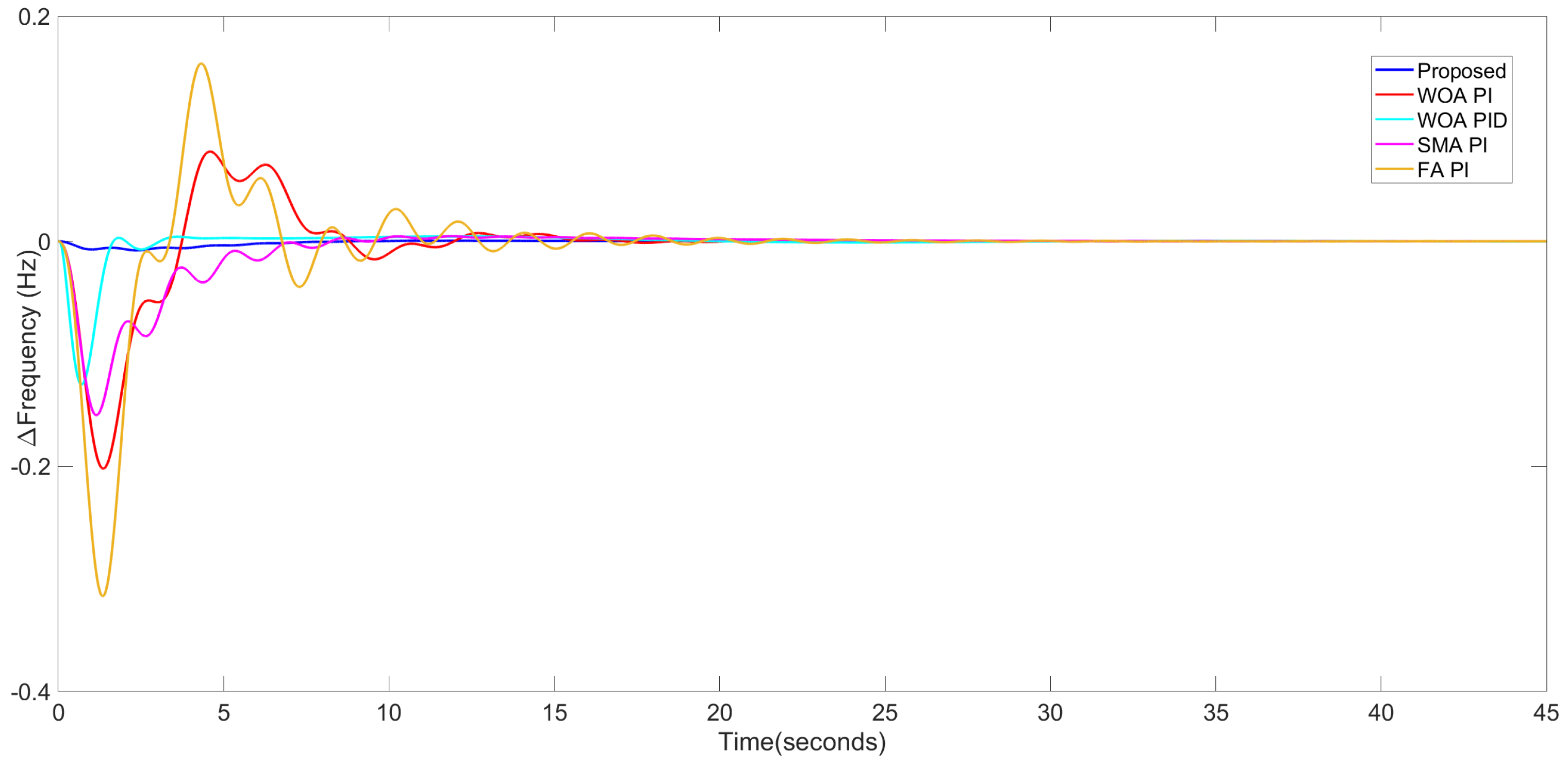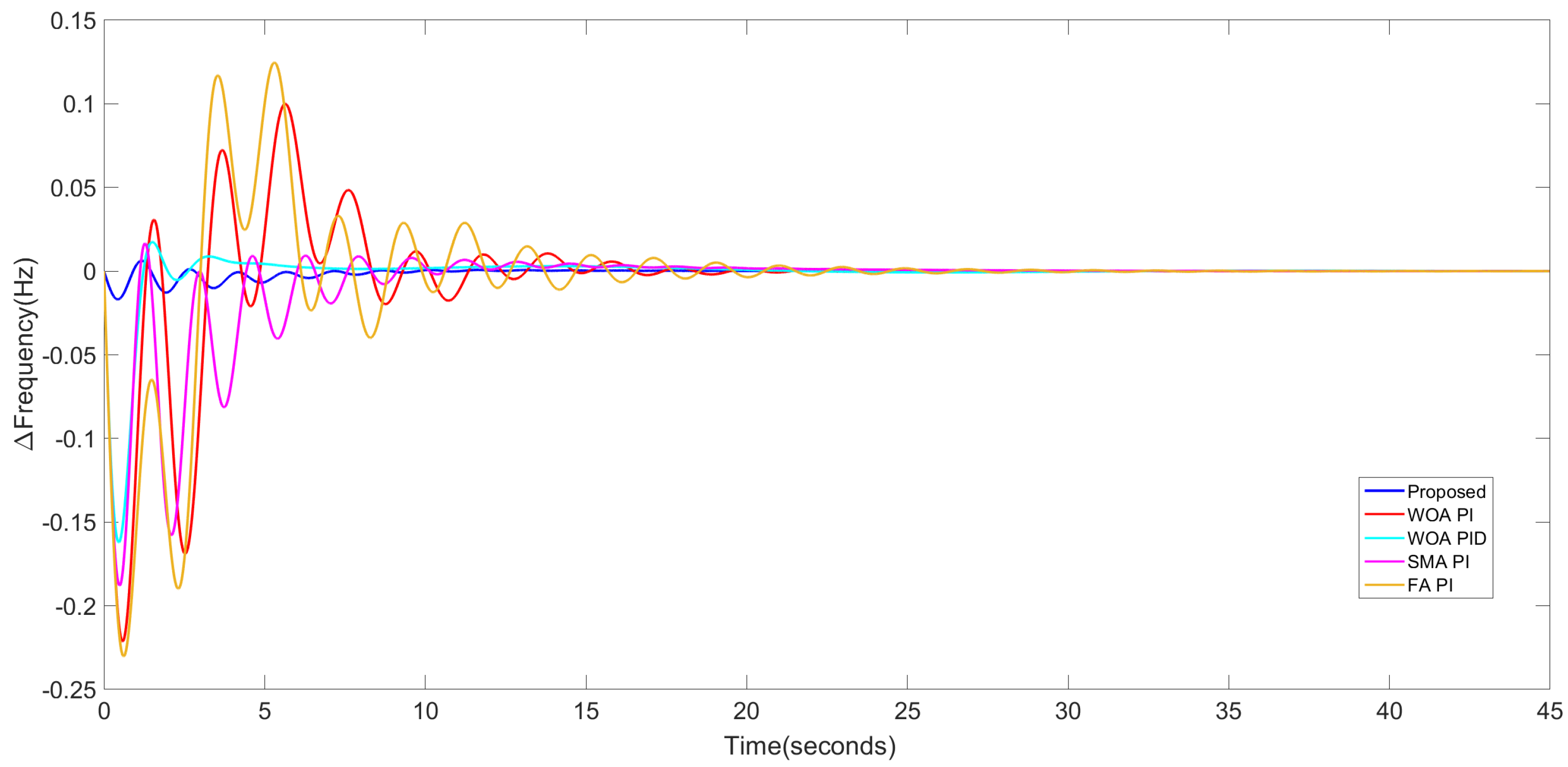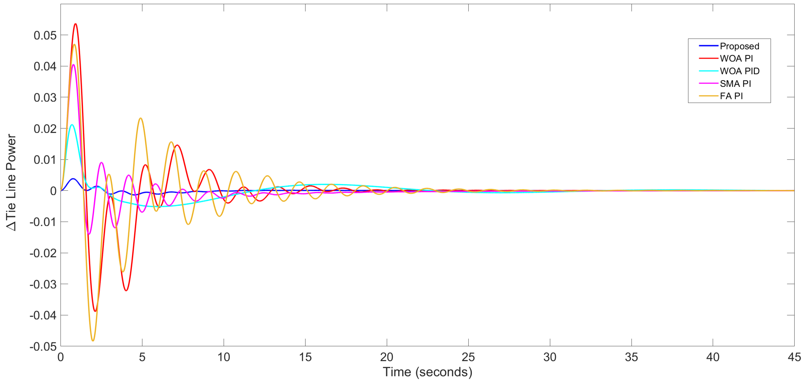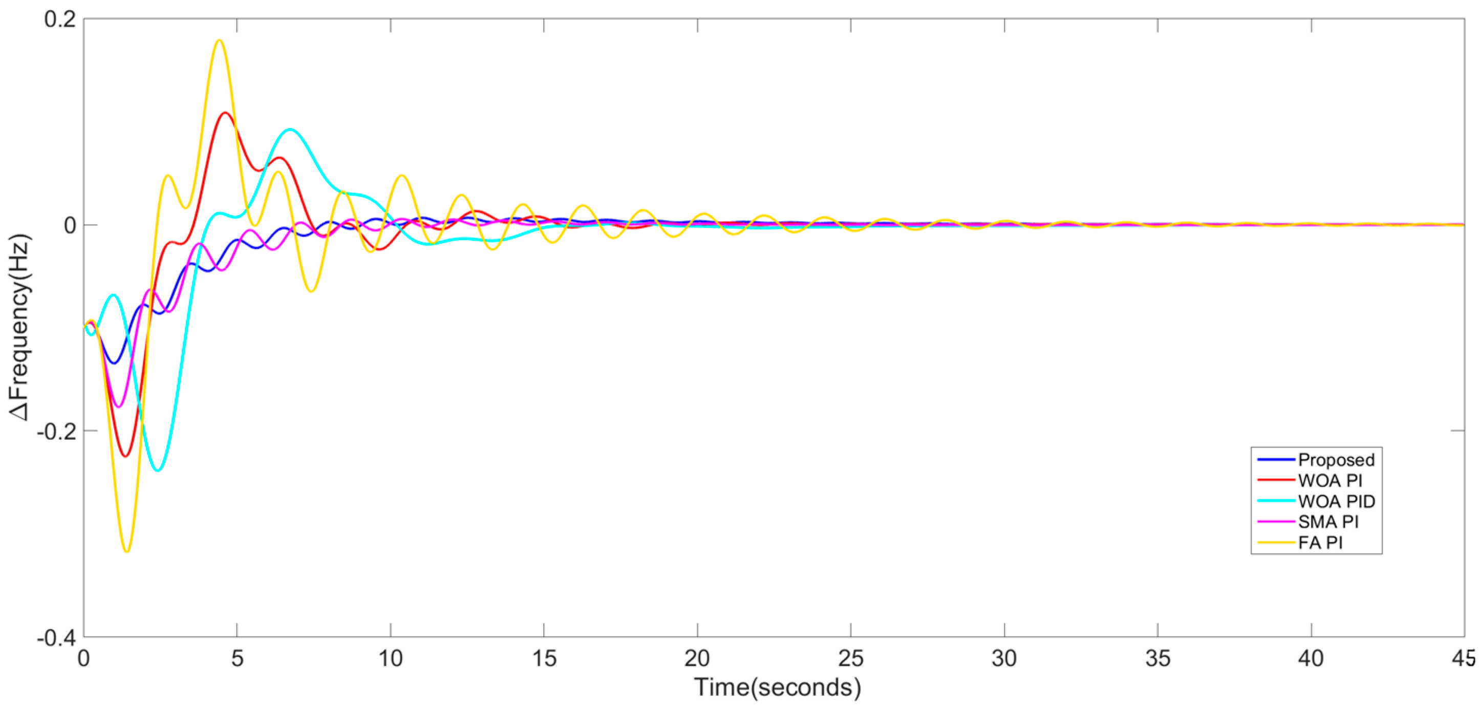The dual-performance metrics are designed to fulfil the WOA optimization technique [39]. We tested with WOA-tuned parameters because of their great convergence speed and accuracy in solving tuning challenges. The simulation findings show that the proposed methods efficiently reduce the frequency and tie-power deviations compared to the classical PI-tuned using the same and other meta-heuristic algorithms.

1.2. Major Contributions

The key contributions to the present work are listed below.

• A focused review is discussed to determine interconnected systems’ types. It can be helpful to see the various control schemes with the LFC method.
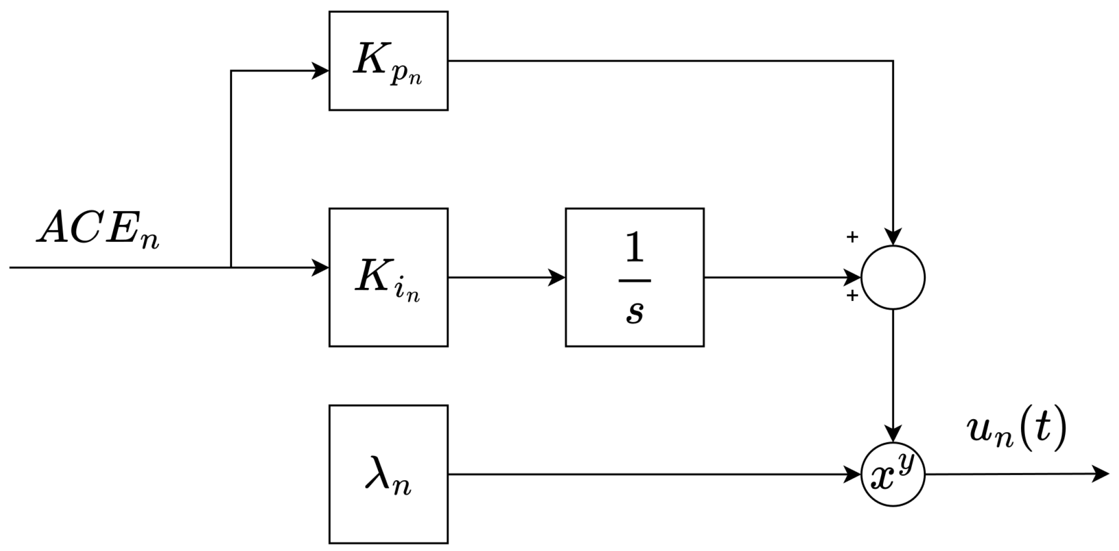
• In contrast to the complicated and big parameter type controllers, a novel tri-parametric fractional-order controller, full-order FO[PI] is provided to demonstrate the advantages over current approaches, i.e., [3,4,5].
• To do this, we create a novel dual-performance index.
• Despite power system nonlinearities, including GRC and GDB, the suggested structure maintains a high level of reliability.
• A modern controller can mitigate the effects of both major changes in system parameters and communication time delay (CTD).

Finally, the rest of the paper is organised as follows. Section 2 describes the power system models simulated in this work. Then, Section 3 concentrates on the design of the proposed scheme. The various investigations are presented in Section 4. Finally, the conclusion is derived under Section 5.

2. PV-RTG Interconnected Hybrid System

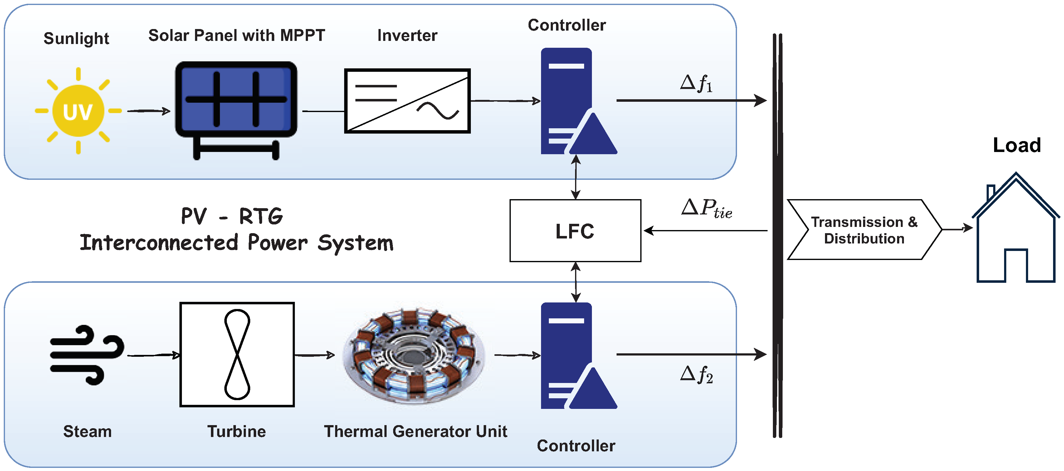
Let us take an application example per the Fiji Islands’ power system architecture. The current real power output is around 112 MW with diesel generators [40]. An alternative can be a hybrid power system to ensure a smooth transition to a renewable energy source, as shown in Figure 1. The first area comprises a solar PV grid of around 50 MW with a high-power solar farm. A second area is a reheated thermal generator having a power output of 62 MW. The voltage output is 240 kV with a frequency of 50 Hz.

The actual description of the power system is difficult and useless for the simulation study due to its nonlinear, time-varying character. Since LFC analysis is based on small-signal modelling, it is necessary to examine a linearly approximated model of the actual power system, as shown in Figure 2. Further study was found in the literature on various control strategies of PV farms to support grid frequency. These controls include synthetic inertia, governor, and AGC control. These approaches were applied to the high PV model effectively [41]. However, the interconnected PV-RTG power system helps to create grid inertia in frequency control in our case. It could be interesting to study the impact of different parameters in PV inertia control and their correlation and impact on frequency response in the future.

From the literature, it has been noted that most presented works have been focused on interconnected power systems having thermal, hydro, and gas. Very little work has been conducted on a hybrid power system combined with PV [3]. The power frequency deviation ($\Delta f$) and the tie-line power deviation ($\Delta P_{tie}$) must return to their rated values during load variations in any area. Therefore, a synthesized measure called area control error (ACE) is used with an LFC as the feedback variable. For the case of two types of power system, each $AC{E}_n$ denotes the nth system ($n=1,2$). In particular, they are defined as below.

$$AC{E}_1\left(s\right)=\Delta P_{tie}+B_1\Delta f_1\left(s\right)$$

(1)

$$AC{E}_2\left(s\right)=-\Delta P_{tie}+B_2\Delta f_2\left(s\right)$$

(2)

The tie-line power deviation from the tie-line exchange power can be calculated as

$$\Delta P_{tie}=\frac{T_{12}}{s}(\Delta f_1-\Delta f_2)$$

(3)

where $T_{12}$ is the tie-line synchronizing coefficient (p.u MW/radian) between PV and RTG measuring the stiffness of the connection and the unit of $\Delta P_{tie}$ is p.u MW. Now for the interconnected power systems, decentralized controllers $C_1\left(s\right)$ and $C_2\left(s\right)$ can be synthesized on the assumption of $\Delta P_{tie}\left(s\right)=0$, as $T_{12}=0$ [20]. Thus, the generalized transfer function for the RTG control area can be written below.

$$G_{RTG}\left(s\right)=B_2\frac{G_{gov}\left(s\right)G_{turb}\left(s\right)P_{re-heat}\left(s\right)G_{genp}\left(s\right)}{1+\frac{G_{gov}\left(s\right)G_{turb}\left(s\right)G_{re-heat}\left(s\right)G_{genp}\left(s\right)}{R}}$$

(4)

where $G_{gov}$, $G_{turb}$, $G_{re-heat}$, and $G_{genp}$ are the transfer functions of the governor, turbine, re-heater, and the generator power systems, respectively. It is noted that this is a generalized transfer function for the scenario when only the thermal system is connected in an interconnected power system. For the chosen work, the scenario is altered with the addition of solar PV. The following subsections discuss the mathematical modeling of each system.

2.1. PV System Model

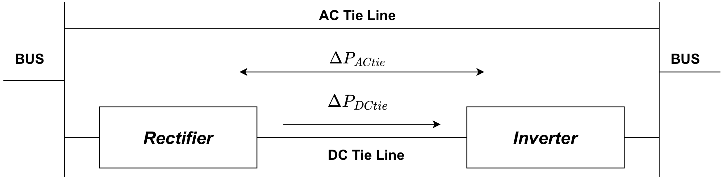
The PV cell model consists of a current source directly proportional to PV array intensity in parallel with a diode and small series contact resistance. The station has an active power rating of 50 MW and comprises 250 PV panels, each with a capacity of 200 KW, according to [42]. The system configuration consists of 50 shunt threads with 5 series panels in each thread. The maximum power point tracking (MPPT) stage and the inverter stage comprise the PV–grid interface. The major goal of the first stage is to ensure that the PV power station operates at peak efficiency using MPPT. The inverter’s primary function is to regulate the power flow between the PV system and the grid. The full mathematical modeling can be found in [5]. Two factors that affect the energy attained from the solar panel are irradiation and temperature. The MPPT algorithm is implemented to achieve maximum efficiency of the PV system. A PV cell is generally shown with current–voltage and power–voltage characteristic curves to understand the effects of temperature and irradiation. Equation (5) gives the total transfer function of the PV system, which includes the PV panel, inverter, MPPT, and filter. The values considered are given in

Table 1. PV and RTG parameters’ values.

PV System	RTG System	Other
$A=-18$	$K_g$ = 1 $T_g$ = 0.08 s	$T_{12}$ = 0.545 p.u MW/radian
$B=900$	$K_t$ = 1 $T_t$ = 0.3 s	$1/R=$ 0.4 Hz/p.u. MW
$C=100$	$K_r$ = 0.33 $T_r$ = 10 s	$B_1$ = $B_2$ = 0.8 p.u. MW/Hz
$D=50$	$K_P$ = 120 $T_P$ = 20 s

. The systems are interconnected via AC tie-line in parallel with HVDC link as shown in Figure 3.

$$G_{PV}\left(s\right)=\frac{As+B}{s^2+Cs+D}$$

(5)

2.2. Thermal System Model

A thermal system consists of a governor, re-heater, turbine, and generator unit. The transfer function equations from (6) to (9) are shown below for each unit.

$$G_{gov}\left(s\right)=\frac{K_g}{s{T}_g+1}$$

(6)

$$G_{tur}\left(s\right)=\frac{K_t}{s{T}_t+1}$$

(7)

$$G_{re-heat}\left(s\right)=\frac{s{K}_r{T}_r+1}{s{T}_r+1}$$

(8)

$$G_{genp}\left(s\right)=\frac{K_P}{s{T}_P+1}$$

(9)

The values of gains and time constants of each component are listed in Table 1.

3. A Fractional-Order Control Scheme

In subnormal system frequency settings, the thermal power plant has the most severe impact. It is possible because the subnormal frequency reduces the blast of induced draught fans and compels the generation power to be reduced. Reduced generator power, for example, can result in a total shutdown. There is little question that with the right controller architecture, the LFC problem may be solved satisfactorily. It is critical to choose suitable time control techniques and structure for the controller.

3.1. Concept Explanation

The structure for the new type of fractional-order controller, namely FO[PI], is written below and illustrated in Figure 4.

$$C_n={\left[K_{p_n}+\frac{K_{i_n}}{s}\right]}^{{\lambda }_n}$$

(10)

Here, $n=1$ or 2 for PV and RTG, respectively. The FO[PI] has $K_{p_n}$, $K_{i_n}$, and non-integral order ${\lambda }_n$ to calculate in the optimization problem. The following literature, [3,4,5], is considered for reference comparisons. It should be noticed that the lowest and upper bounds for tuning $\lambda$ have been set to zero and two, respectively. The selection of these relatively small values is based on the research given in [21]. It demonstrates that a high order value may have an impact on the system’s stability.

As with the case of any controller, tuning to obtain the optimal parameters is paramount. A total of six parameters are to be tuned as per the studied hybrid interconnected systems. Choosing a competent method is necessary. As shown in the literature, meta-heuristic algorithms are very popular and efficient. In particular, Particle Swarm Optimization (PSO) is a widely and commonly used algorithm. However, the proposed scheme uses the Whale Optimization Algorithm (WOA) due to the fact that it is quite robust to global optimization. The swarm intelligence optimization algorithm, WOA, replicates humpback whale hunting. The program mimics whale predatory behaviour to tackle the goal problem [39]. The updated pseudo-code steps as per the designed optimization index are presented in

Table 2. The pseudo-code for dual optimization.

Initialize the whale’s population

Set algorithm parameters vector ($\eta$)

Set performance index (11)

Calculate the fitness of all search agents

While (termination criteria not satisfied)

Encircle prey

Bubble net hunt

Search the prey

Compute the dual fitness value (13)

End While

Return the best result ($\eta *$)

End

.

3.2. Dual Performance Measure for Tuning

Parameter settings are crucial when constructing a controller. LFC for a two-area power system should include a target function that optimizes parameters for quick responsiveness, quicker settling time, and minimized overshoot. In real life, large variations in the control signal might increase expenses and maintenance [43]. Excessive power system activity may create valve or actuator motions that wear or break mechanical components such as springs or linkages. Thus, optimal settings involve checking controller output variations.

The dual performance requirement is imposed while developing the proposed controller. The first measure minimizes the Integral Squared Time Error (ISTE) criterion. The ISTE is chosen due to its ability to penalize significant errors since the square of a large error will be much more meaningful. The ISTE index can be described below.

$$J_{ISTE}\left(\eta \right)=\underset{0}{\overset{\infty }{\int }}{\left(te(\eta ,t)\right)}^2\mathrm{dt}$$

(11)

where $\eta$ is a set of parameters to obtain optimally. The second requirement is enforced together to restrict the control signal output. Analytically, it can be indexed as below.

$$J_u=\underset{\eta }{min}\underset{0}{\overset{\infty }{\int }}\left|\frac{du}{dt}\right|\mathrm{dt}$$

(12)

The controller’s smoothness and low input utilization (energy) are seen as indicators of its quality, resulting in lower total system maintenance costs. As per the PV-RTG system in this work, the controller will be designed to satisfy both criteria stated in (11) and (12). The new performance measure as per LFC problem is therefore defined as follows.

$$\begin{array}{c}{J}_{ISTE}=\underset{{\eta }^{*}}{min}\underset{0}{\overset{\infty }{\int }}[{\left(tAC{E}_1\right)}^2+{\left(tAC{E}_2\right)}^2]\mathrm{dt}\hfill \\ \mathrm{subject}\mathrm{to}{J}_u=\underset{{\eta }^{*}}{min}\underset{0}{\overset{\infty }{\int }}\left|\frac{du}{dt}\right|\mathrm{dt}\hfill \end{array}$$

(13)

where $\Delta f_1\left(t\right)$ and $\Delta f_2\left(t\right)$ are the changes in frequency in PV and RTG systems, respectively. $\Delta P_{tie}\left(t\right)$ is the tie-line power change. The vector ${\eta }^{*}$ is the optimal values of parameters calculated using the WOA algorithm. Note that ${\eta }^{*}$ has parameters $K_{p1}$, $K_{i1}$, ${\lambda }_1$, $K_{p2}$, $K_{i2}$, and ${\lambda }_2$.

In the following section, the results obtained from the new controller structure and dual performance index in (13) are presented. The results are compared with the latest methods presented by Shakibjoo et al. [3], Khamies et al. [4] and Abd-Elazim and Ali [5].

4. Validations

4.1. Implementation of the System Model and WOA

The model of the system, as shown in Figure 2, is developed in a MATLAB/Simulink^® environment at the computer including Intel^® core™ i7 at 2.60 GHz 2.81 GHz CPU and 8 GB RAM. The WOA has been set up with the number of search agents as 1, and iterations are chosen as 50. These parameters’ upper and lower bounds have been chosen as −2 and 2, respectively. The developed model is simulated in a separate program (by .m file using initial population/controller parameters) and via Simulink, considering conditions discussed in the subsections below. The objective function for each individual is calculated in another program’s power system model (*.mdl file) and transferred to a MATLAB file through the workspace. The objective function in (13) was used as the performance measure to evaluate the populations. After a fixed number of iterations, the best parameters are obtained as given in

Table 3. Estimated controller parameters for studied hybrid power system.

Parameter	Proposed WOA FO[PI]	WOA PI [3]	WOA PID [3]	SMA PI [4]	FA PI [5]
$K_{p1}$	−0.225	−0.225	−0.107	−0.056	−0.577
$K_{i1}$	−0.056	−0.456	−0.091	−0.619	−0.881
${\lambda }_1$	0.952	1.000	−0.611	1.000	1.000
$K_{p2}$	−2.124	−0.987	−1.894	−0.472	−0.831
$K_{i2}$	−0.310	−0.897	−1.894	−1.999	−0.763
${\lambda }_2$	0.825	1.000	−0.251	1.000	1.000

.

4.2. Analysis

Verifying the performance with various situations, measurement parameters, and analysis is important. The parameters from recently published and from the proposed techniques are given in Table 3. Note that the second, third, and fourth columns in the table show the values given by other methods. We note again that [3] used the same WOA; [4] used the Slime Mould Algorithm (SMA); and [5] used the Firefly Algorithm (FA) for the tuning and optimizing the PI parameter values. In all comparative plots, we have shown the FO[PI] as Proposed, Shakibjoo et al.’s [3] approaches as WOA PI and WOA PID, Khamies et al. [4] as SMA-PI and Abd-Elazim and Ali [5] as FA PI. For these references, the same interconnected PV-RTG power system model was verified. To establish the acceptance of the proposed method, major analyses have been conducted, which are disturbance analysis and parameter perturbation analysis. In addition, we have considered a practical condition of the power system’s non-linearity as physical limitations such as GRC and GDB in the analysis. Furthermore, a time delay with a value of half a second is added on both control action and control input with the same parameters as in Table 3.

4.2.1. Disturbance Analysis

The disturbance input analysis is key verification for any controller design. This analysis assesses how the closed-loop system behaves to step disturbances. A disturbance signal denoted by $\Delta Load$ is injected in both PV and RTG. In order to verify the performance, a constant step input and a dynamic load perturbation (DLP) are used in the analysis. This way, a total of three scenarios has been established. Scenario-1 is conducted with 0.1 pu step disturbance in the RTG system. Scenario-2 verifies with 0.1 pu step disturbances in PV and RTG simultaneously. Finally, Scenario-3 tests a dynamic load perturbation using the test signal shown in Figure 5.

Scenario 1: Change in Demand of RTG System

A 10% step increase in demand of RTG system has been used. The output responses are shown in Figure 6, Figure 7 and Figure 8. The comparison investigation shows that the provided technique outperforms [3,4,5] methods.

Table 4. Scenario 1 Numerical Study.

Methods	Peak Overshoot (×10${}^{-2}$)			Peak Undershoot (×10${}^{-2}$)			Settling Time (s)
	$\Delta {\mathit{f}}_{\mathbf{1}}$	$\Delta {\mathit{f}}_{\mathbf{2}}$	$\Delta {\mathit{P}}_{\mathit{tie}}$	$\Delta {\mathit{f}}_{\mathbf{1}}$	$\Delta {\mathit{f}}_{\mathbf{2}}$	$\Delta {\mathit{P}}_{\mathit{tie}}$	$\Delta {\mathit{f}}_{\mathbf{1}}$	$\Delta {\mathit{f}}_{\mathbf{2}}$	$\Delta {\mathit{P}}_{\mathit{tie}}$
Proposed WOA FO[PI]	0.326	5.462	3.865	−8.613	−16.920	−1.160	17.866	19.875	22.738
WOA PI [3]	7.977	9.949	5.366	−20.200	−22.110	−3.883	32.016	32.066	30.785
WOA PID [3]	4.720	5.183	6.920	−16.960	−18.060	−2.729	24.073	23.172	22.738
SMA PI [4]	0.459	18.790	4.053	−15.460	−18.790	−1.403	21.797	21.508	28.781
FA PI [5]	15.810	12.470	4.704	−31.550	−23.020	−4.835	28.932	32.673	41.749

also suggests that the new structure outperforms others in overshoot, undershoot, and settling time. Note that FO[PI] is superior to the same tree-parameters scheme of PID, with the same optimization method, WOA.

Nevertheless, the presented structure worked well with the improved responses. Measuring the value of fluctuations in the controller outputs is also required. As discussed in Section 3.2, the supremacy of the dual performance index (13) is reflected in the plotted values in Figure 9. It is observed that the input of the plants varies much less than others. It is therefore confirmed that the proposed controller can minimize the variations in the controller’s output; thus, it will reduce the maintenance cost and wear of moving parts.

Scenario 2: Change in Demand in Both Areas

In this verification, let us take 10% increase in demand from both areas. The results are shown in Figure 10, Figure 11 and Figure 12.

Table 5. Scenario 2 Numerical Study.

Methods	Peak Overshoot (×10${}^{-2}$)			Peak Undershoot (×10${}^{-2}$)			Settling Time (s)
	$\Delta {\mathit{f}}_{\mathbf{1}}$	$\Delta {\mathit{f}}_{\mathbf{2}}$	$\Delta {\mathit{P}}_{\mathit{tie}}$	$\Delta {\mathit{f}}_{\mathbf{1}}$	$\Delta {\mathit{f}}_{\mathbf{2}}$	$\Delta {\mathit{P}}_{\mathit{tie}}$	$\Delta {\mathit{f}}_{\mathbf{1}}$	$\Delta {\mathit{f}}_{\mathbf{2}}$	$\Delta {\mathit{P}}_{\mathit{tie}}$
Proposed WOA FO[PI]	0.364	0.600	1.785	−13.100	−20.000	−2.015	17.001	19.270	18.143
WOA PI [3]	9.754	10.180	3.772	−21.930	−26.710	−4.761	31.145	33.483	38.743
WOA PID [3]	5.336	5.108	4.233	−19.130	−22.940	−4.124	23.168	23.605	39.516
SMA PI [4]	0.255	0.527	2.344	−15.300	−22.390	−2.293	22.442	23.012	50.000
FA PI [5]	15.670	13.770	3.642	−30.640	−27.570	−5.056	28.798	38.271	40.159

shows the measured values from all methods. Again, the presented controller works better than the recently reported controllers. In summary, the fractional-order controller is suitable for the stated system. It rejects disturbances best by returning to the original state fastest in both circumstances. From the results, it is also noted that the proposed FO[PI] is capable of providing minimum overshoot and undershoot.

Scenario 3: Dynamic Load Perturbation Test

The results presented in the above two scenarios are based on unit step load perturbation. However, in an actual power system, all the control areas simultaneously experience various load changes and magnitudes at different times. Taking that into consideration, for PV, 5% pulse width load is injected at 57 s, and in RTG, −10% step load is injected at 30 s. Such a disturbance signal is illustrated in Figure 5. The deviations verify the affirmation of robustness regarding disturbance rejection to the frequency and tie-line power. The results are illustrated in Figure 13, Figure 14 and Figure 15. It has been observed that the whole system approached a steady-state value more speedily with the proposed controllers than the other controllers. This compatibility handles the projected multiple load changes and significantly improves system performance.

It is noted from all three scenarios that the FO[PI] controller has performed better with respect to settling time value. For a fair comparison, the controller values are calculated from the exact initial guess and the number of iterations from WOA. It is required to claim efficacy with a simple FO[PI] controller. Though the structure of FO[PI] has three parameters to tune, such as FOPI and PID, it has a lower settling time than all previous structures; thus, the system’s output obtained a steady-state value quickly. As per the result, one can claim that the FO[PI] is better than others with respect to settling time.

4.2.2. Parameter Perturbation Analysis

Parameter perturbation studies mimic actual situations where plant parameters may change after initial setup. Small parameter changes can trigger major power system breakdowns. RTG settings are adjusted accordingly. These modifications are limited to the nominal parameter values’ permissible range. Thus, we considered it as shown in

Table 6. Considered parameter perturbations.

Case No.	${\mathit{T}}_{\mathit{g}}$ Variation	${\mathit{T}}_{\mathit{t}}$ Variation
Case 1	+40%	+40%
Case 2	−40%	−40%

. The 40% increase and decrease in the Governor Time ($T_g$) and Turbine Time ($T_t$) constants are considered.

Perturbed Governor Time Constant

Case 1: 40% increased ${\mathbf{T}}_{\mathbf{g}}$ value

The responses with the same methods are shown in Figure 16, Figure 17 and Figure 18.

Table 7. Response data for Case 1 in $T_g$.

Methods	Increase by 40%
	Peak Overshoot (×10${}^{-\mathbf{2}}$)			Peak Undershoot (×10${}^{-\mathbf{2}}$)			Settling Time
	$\Delta {\mathit{f}}_{\mathbf{1}}$	$\Delta {\mathit{f}}_{\mathbf{2}}$	$\Delta {\mathit{P}}_{\mathit{tie}}$	$\Delta {\mathit{f}}_{\mathbf{1}}$	$\Delta {\mathit{f}}_{\mathbf{2}}$	$\Delta {\mathit{P}}_{\mathit{tie}}$	$\Delta {\mathit{f}}_{\mathbf{1}}$	$\Delta {\mathit{f}}_{\mathbf{2}}$	$\Delta {\mathit{P}}_{\mathit{tie}}$
Proposed WOA FO[PI]	0.808	3.559	2.051	−13.670	−21.200	−2.388	22.565	37.695	29.167
WOA PI [3]	11.040	12.460	4.008	−22.830	−27.600	−5.315	28.211	39.342	32.926
WOA PID [3]	5.535	5.737	4.509	−19.63	−23.65	−4.327	23.772	25.340	41.337
SMA PI [4]	0.671	3.101	2.570	−17.990	−23.320	−2.767	26.703	38.779	39.429
FA PI [5]	17.550	16.020	3.827	−31.880	−28.430	−5.492	34.332	39.646	40.600

gives the numerical comparison values. In the tested cases, the proposed controllers perform well under perturbations and do not give noticeable oscillations, which can cause major disruptions.

Case 2: 40% decreased ${\mathit{T}}_{\mathit{g}}$ value

Again, the responses with the same methods are shown in Figure 19, Figure 20 and Figure 21.

Table 8. Response data for Case 2 in $T_g$.

Methods	Increase by 40%
	Peak Overshoot (×10${}^{-\mathbf{2}}$)			Peak Undershoot (×10${}^{-\mathbf{2}}$)			Settling Time
	$\Delta {\mathit{f}}_{\mathbf{1}}$	$\Delta {\mathit{f}}_{\mathbf{2}}$	$\Delta {\mathit{P}}_{\mathit{tie}}$	$\Delta {\mathit{f}}_{\mathbf{1}}$	$\Delta {\mathit{f}}_{\mathbf{2}}$	$\Delta {\mathit{P}}_{\mathit{tie}}$	$\Delta {\mathit{f}}_{\mathbf{1}}$	$\Delta {\mathit{f}}_{\mathbf{2}}$	$\Delta {\mathit{P}}_{\mathit{tie}}$
Proposed WOA FO[PI]	0.353	0.286	7.628	−12.570	−18.990	−6.733	24.906	19.747	22.262
WOA PI [3]	8.698	8.405	3.525	−21.100	−25.730	−4.310	28.418	25.296	37.999
WOA PID [3]	5.205	4.697	4.000	−18.680	−22.130	−3.998	26.250	35.267	44.588
SMA PI [4]	0.295	0.197	2.099	−16.340	−21.210	−1.863	24.998	20.484	44.371
FA PI [5]	13.940	11.710	3.439	−29.390	−26.560	−4.631	27.724	24.386	31.366

gives the numerical comparison values. In the tested cases, the proposed controllers perform well under perturbations and do not give noticeable oscillations which can cause major disruptions.

Perturbed Turbine Time Constant

Case 1: 40% increased ${\mathit{T}}_{\mathit{t}}$ value

The nominal value response is compared to the cases mentioned earlier. Figure 22, Figure 23 and Figure 24 are shown with perturbed responses in all cases in both areas.

Table 9. Response data for Case 1 in $T_t$.

Methods	Increase by 40%
	Peak Overshoot (×10${}^{-\mathbf{2}}$)			Peak Undershoot (×10${}^{-\mathbf{2}}$)			Settling Time
	$\Delta {\mathit{f}}_{\mathbf{1}}$	$\Delta {\mathit{f}}_{\mathbf{2}}$	$\Delta {\mathit{P}}_{\mathit{tie}}$	$\Delta {\mathit{f}}_{\mathbf{1}}$	$\Delta {\mathit{f}}_{\mathbf{2}}$	$\Delta {\mathit{P}}_{\mathit{tie}}$	$\Delta {\mathit{f}}_{\mathbf{1}}$	$\Delta {\mathit{f}}_{\mathbf{2}}$	$\Delta {\mathit{P}}_{\mathit{tie}}$
Proposed WOA FO[PI]	1.036	4.598	2.389	−14.510	−22.220	−2.851	27.522	34.289	35.918
WOA PI [3]	13.360	14.810	4.342	−24.300	−28.540	−6.024	32.392	39.634	39.733
WOA PID [3]	6.968	8.795	5.052	−20.830	−24.880	−5.156	30.927	35.582	39.689
SMA PI [4]	1.148	4.490	2.886	−93.500	−24.160	−3.250	33.211	35.366	42.117
FA PI [5]	20.610	18.780	4.083	−34.050	−29.430	−5.970	39.375	41.746	43.634

gives the numerical comparison values. Again, it is clear to say that under this condition, the proposed method also resulted in an excellent output.

Case 2: 40% decreased ${\mathit{T}}_{\mathit{t}}$ value

Nominal responses are compared to the cases mentioned earlier. Figure 25, Figure 26 and Figure 27 are given with perturbed outputs in all cases in both areas.

Table 10. Response data for Case 2 in $T_t$.

Methods	Decrease by 40%
	Peak Overshoot (×10${}^{-\mathbf{2}}$)			Peak Undershoot (×10${}^{-\mathbf{2}}$)			Settling Time
	$\Delta {\mathit{f}}_{\mathbf{1}}$	$\Delta {\mathit{f}}_{\mathbf{2}}$	$\Delta {\mathit{P}}_{\mathit{tie}}$	$\Delta {\mathit{f}}_{\mathbf{1}}$	$\Delta {\mathit{f}}_{\mathbf{2}}$	$\Delta {\mathit{P}}_{\mathit{tie}}$	$\Delta {\mathit{f}}_{\mathbf{1}}$	$\Delta {\mathit{f}}_{\mathbf{2}}$	$\Delta {\mathit{P}}_{\mathit{tie}}$
Proposed WOA FO[PI]	0.334	0.276	1.073	−11.640	−17.230	−1.251	18.403	23.996	37.218
WOA PI [3]	6.820	6.366	3.068	−19.300	−24.200	−3.380	21.221	25.123	39.386
WOA PID [3]	4.674	3.757	3.421	−17.450	−20.470	−3.580	24.473	30.542	43.374
SMA PI [4]	0.192	0.134	1.688	−14.750	−19.810	−1.177	20.788	22.526	45.000
FA PI [5]	10.650	8.378	3.070	−26.750	−25.110	−3.840	24.776	24.863	30.802

gives the numerical comparison values. Again, it is proved that the new (PI)${}^{\lambda }$ has better robustness, even in the presence of maximum parameter changes.

4.2.3. Stability Analysis with Nonlinearities

With some challenges, let us validate the proposed scheme’s stability and effectiveness. The nonlinearities such as GRC and GDB have been added to area-2 (RTG system). The steam turbine’s thermodynamics and mechanical parts create the GRC, whereas the hydraulic relay’s overlapping values, backlash, and linkage friction cause the GDB [6]. In the presence of such nonlinearities, the proposed scheme resulted in better quality, as shown in Figure 28, Figure 29 and Figure 30. It is worth claiming that the proposed (PI)${}^{\lambda }$ handles the effects of GBC and GDB with less overshoot and undershoot.

Table 11. Results with non-linearities.

Methods
	Peak Overshoot (×10${}^{-\mathbf{2}}$)			Peak Undershoot (×10${}^{-\mathbf{2}}$)			Settling Time
	$\Delta {\mathit{f}}_{\mathbf{1}}$	$\Delta {\mathit{f}}_{\mathbf{2}}$	$\Delta {\mathit{P}}_{\mathit{tie}}$	$\Delta {\mathit{f}}_{\mathbf{1}}$	$\Delta {\mathit{f}}_{\mathbf{2}}$	$\Delta {\mathit{P}}_{\mathit{tie}}$	$\Delta {\mathit{f}}_{\mathbf{1}}$	$\Delta {\mathit{f}}_{\mathbf{2}}$	$\Delta {\mathit{P}}_{\mathit{tie}}$
Proposed WOA FO[PI]	0.043	0.622	0.381	−0.810	−1.688	−0.138	15.436	19.270	18.143
WOA PI [3]	7.930	9.990	5.362	−20.180	−22.020	−3.877	27.229	25.166	32.666
WOA PID [3]	0.404	1.734	2.119	−12.730	−16.210	−0.512	22.399	19.790	35.311
SMA PI [4]	0.443	1.662	4.035	−15.460	−18.71	−1.390	32.059	28.895	28.084
FA PI [5]	15.810	12.430	4.668	−31.440	−23.000	−4.820	36.246	30.238	39.001

shows the numerical supremacy of the proposed schemes over the reported works. The frequency and tie-line power can settle to steady-state values quickly and retain the system’s stability.

4.2.4. Addition of Communication Time Delays

To investigate further, a communication time delay (CTD) with a value of half a second is added before and after the controllers, as seen in Figure 2. This test aims to ascertain whether the delay impulsively affects the time response of the whole system.

Table 12. Results after considering communication delays.

Methods
	Peak Overshoot (×10${}^{-\mathbf{2}}$)			Peak Undershoot (×10${}^{-\mathbf{2}}$)			Settling Time
	$\Delta {\mathit{f}}_{\mathbf{1}}$	$\Delta {\mathit{f}}_{\mathbf{2}}$	$\Delta {\mathit{P}}_{\mathit{tie}}$	$\Delta {\mathit{f}}_{\mathbf{1}}$	$\Delta {\mathit{f}}_{\mathbf{2}}$	$\Delta {\mathit{P}}_{\mathit{tie}}$	$\Delta {\mathit{f}}_{\mathbf{1}}$	$\Delta {\mathit{f}}_{\mathbf{2}}$	$\Delta {\mathit{P}}_{\mathit{tie}}$
Proposed WOA FO[PI]	0.120	2.034	2.088	0.091	−0.026	−2.347	32.184	19.270	33.389
WOA PI [3]	0.139	14.000	3.999	−0.016	−0.036	−5.249	33.577	25.166	37.096
WOA PID [3]	9.225	7.963	4.495	−0.104	−0.169	−5.676	45.000	19.790	45.000
SMA PI [4]	0.540	2.934	2.563	−0.0455	−0.2010	−2.703	45.000	28.895	45.000
FA PI [5]	0.179	16.500	3.877	−0.387	−0.288	−5.621	45.000	30.238	45.000

shows the numerical supremacy of the proposed scheme over the reported works. For reference, the response outputs are provided further by Figure 31, Figure 32 and Figure 33. It can be seen that the proposed (PI)${}^{\lambda }$ could be significantly robust with CTD compared to other control strategies.

5. Conclusions

The impact of PV systems on LFC design problems has received the least attention in the literature. In this research, the entire fractional-order structure like (PI)${}^{\lambda }$ (FO[PI]) was examined for the resilience of power systems from load demand changes and parameter perturbations. This paper studied the LFC problem using dual performance indices and fewer tuning factors. Regarding settling time, the chosen application of a two-interconnected hybrid power system performed better with the fractional-order structure than previously reported techniques. On average, the settling time was shortened by 30%. For real applications, frequency and power output responses oscillate where the proposed technique can reduce those oscillations effectively. More crucially, the system has improved its stability, ensuring strong performance in the face of parameter disruptions and uncertainty. Later, the performance of the primary fractional controller with nonlinearity and communication delay is investigated. Finally, the analysis in this paper validated the efficacy and flexibility of a primary three-parameter fractional-order controller.

Similarly, future works can use a less complex controller to study the LFC problem on a multi-area energy network. It is also possible to modify the presented controller using two or three degrees of freedom with or without a fractional-order setpoint filter to achieve further robustness and faster responses. A similar study can be a future scope considering a less computational burden.

References

1. Guha, D.; Roy, P.; Banerjee, S. Disturbance observer aided optimised fractional-order three degree of freedom tilt integral derivative controller for load frequency control of power systems. IET Gener. Transm. Distrib. 2020, 15, 716–736. [Google Scholar] [CrossRef]
2. Elgerd, O.I.; Happ, H.H. Electric Energy Systems Theory: An Introduction. IEEE Trans. Syst. Man Cybern. 1972, SMC-2, 296–297. [Google Scholar] [CrossRef]
3. Shakibjoo, A.; Kumar, A.; Panda, S. A novel modified whale optimization algorithm for load frequency controller design of a two-area power system composing of PV grid and thermal generator. Neural Comput. Appl. 2020, 32, 8205–8216. [Google Scholar] [CrossRef]
4. Khamies, M.; Magdy, G.; Kamel, S.; Elsayed, S. Slime Mould Algorithm for Frequency Controller design of two-area thermal-PV power system. In Proceedings of the IEEE International Conference on Automation/XXIV Congress of the Chilean Association of Automatic Control (ICA-ACCA), Valparaíso, Chile, 22–26 March 2021; Volume 11, pp. 623–635. [Google Scholar] [CrossRef]
5. Abd-Elazim, S.; Ali, E. Load Frequency controller design of a two-area system composing of PV grid and thermal generator via firefly algorithm. Neural Comput. Appl. 2018, 30, 607–616. [Google Scholar] [CrossRef]
6. Guha, D.; Roy, P.; Banerjee, S. Whale optimization algorithm applied to load frequency control of a mixed power system considering nonlinearities and PLL dynamics. Energy Syst. 2020, 11, 699–728. [Google Scholar] [CrossRef]
7. Guha, D.; Roy, P.; Banerjee, S. Performance evolution of different controllers for frequency regulation of a hybrid energy power system employing chaotic crow search algorithm. ISA Trans. 2021, 120, 128–146. [Google Scholar] [CrossRef] [PubMed]
8. Sariki, M.; Shankar, R. Optimal CC-2DOF(PI)-PDF controller for LFC of restructured multi-area power system with IES-based modified HVDC tie-line and electric vehicles. Eng. Sci. Technol. Int. J. 2022, 32, 101058–101072. [Google Scholar] [CrossRef]
9. Poulose, A.; Ramesh, K. Super-Twisting Algorithm based Load Frequency Control of a Two Area Interconnected Power System. In Proceedings of the 2019 20th International Conference on Intelligent System Application to Power Systems (ISAP), New Delhi, India, 10–14 December 2019; pp. 1–5. [Google Scholar] [CrossRef]
10. Debbarma, S.; Saikia, L.C.; Sinha, N. AGC of a multi-area thermal system under deregulated environment using a non-integer controller. Electr. Power Syst. Res. 2013, 95, 175–183. [Google Scholar] [CrossRef]
11. Pradhan, P.; Sahu, R.; Panda, S. Firefly algorithm optimized fuzzy PID controller for AGC of multi-area multi-source power systems with UPFC and SMES. Eng. Sci. Technol. Int. J. 2016, 19, 338–354. [Google Scholar] [CrossRef]
12. Sahu, R.; Panda, S.; Pradhan, P. Design and analysis of hybrid firefly algorithm-pattern search based fuzzy PID controller for LFC of multi area power systems. Int. J. Electr. Power Energy Syst. 2015, 69, 200–212. [Google Scholar] [CrossRef]
13. Shankar, G.; Mukherjee, V. Quasi oppositional harmony search algorithm based controller tuning for load frequency control of multi-source multi-area power system. Int. J. Electr. Power Energy Syst. 2016, 75, 289–302. [Google Scholar] [CrossRef]
14. Abo-Elyousr, F.K. Load frequency controller design for two area interconnected power system with DFIG based wind turbine via ant colony algorithm. In Proceedings of the 2016 Eighteenth International Middle East Power Systems Conference (MEPCON), Cairo, Egypt, 27–29 December 2016; pp. 253–260. [Google Scholar] [CrossRef]
15. Padiachy, V.; Mehta, U.; Azid, S.; Prasad, S.; Kumar, R. Two degree of freedom fractional PI scheme for automatic voltage regulation. Eng. Sci. Technol. Int. J. 2021, 30, 101046. [Google Scholar] [CrossRef]
16. Oshnoei, S.; Oshnoei, A.; Haghjoo, F. Novel load frequency control scheme for an interconnected two-area power system including wind turbine generation and redox flow battery. Int. J. Electr. Power Energy Syst. 2021, 130, 107033. [Google Scholar] [CrossRef]
17. Singh, J.; Chatterjee, K.; Vishwakarma, C.B. Two degree of freedom internal model control-PID design for LFC of power systems via logarithmic approximations. ISA Trans. 2018, 72, 185–196. [Google Scholar] [CrossRef] [PubMed]
18. Zamani, A.; Barakati, S.; Darmian, S. Design of a fractional order PID controller using GBMO algorithm for load–frequency control with governor saturation consideration. ISA Trans. 2016, 64, 56–66. [Google Scholar] [CrossRef]
19. Morsali, J.; Zare, K.; Hagh, M. Applying fractional order PID to design TCSC-based damping controller in coordination with automatic generation control of interconnected multi-source power system. Eng. Sci. Technol. Int. J. 2021, 20, 578–588. [Google Scholar] [CrossRef]
20. Saxena, S. Load frequency control strategy via fractional-order controller and reduced-order modeling. Int. J. Electr. Power Energy Syst. 2019, 104, 603–614. [Google Scholar] [CrossRef]
21. Mehta, U.; Lechappe, V.; Singh, O.P. Simple FOPI tuning method for real-order time delay systems. In Advances in Systems, Control and Automation; Springer: Berlin/Heidelberg, Germany, 2018; pp. 459–468. [Google Scholar]
22. Shankaran, V.P.; Azid, S.I.; Mehta, U. Fractional-order PI plus D controller for second-order integrating plants: Stabilization and tuning method. ISA Trans. 2022, 129, 592–604. [Google Scholar] [CrossRef]
23. Abo-Elyousr, F.K.; Sharaf, A.M. A novel modified robust load frequency controller scheme. Energy Syst. 2020, 11, 1175–1198. [Google Scholar] [CrossRef]
24. Singh, K.; Arya, Y. Jaya-ITDF control strategy-based frequency regulation of multi-microgrid utilizing energy stored in high-voltage direct current-link capacitors. Soft Comput. 2023, 27, 5951–5970. [Google Scholar] [CrossRef]
25. Zhang, G.; Khan, I.A.; Daraz, A.; Basit, A.; Khan, M.I. Load Frequency Control of Marine Microgrid System Integrated with Renewable Energy Sources. J. Mar. Sci. Eng. 2023, 11, 844. [Google Scholar] [CrossRef]
26. Khadanga, R.; Moradzadeh, M.; Moussavi, S.Z.; Mohammadzadeh, A.; Vandevelde, L. Load frequency control for multi-area power systems: A new type-2 fuzzy approach based on Levenberg–Marquardt algorithm. ISA Trans. 2021, 21, 40–52. [Google Scholar] [CrossRef]
27. Khadanga, R.; Kumar, A.; Panda, S. Frequency control in hybrid distributed power systems via type-2 fuzzy PID controller. IET Renew. Power Gener. 2021, 15, 1706–1723. [Google Scholar] [CrossRef]
28. Meziane, K.; Naoual, P.; Boumhidi, I. Type-2 Fuzzy Logic based on PID controller for AGC of Two-Area with Three Source Power System including Advanced TCSC. Procedia Comput. Sci. 2019, 148, 455–464. [Google Scholar] [CrossRef]
29. Ismail, M.; Bendary, A. Load Frequency Control for Multi Area Smart Grid based on Advanced Control Techniques. Alex. Eng. J. 2018, 57, 4021–4032. [Google Scholar] [CrossRef]
30. Lone, A.; Yousuf, V.; Prakash, S.; Bazaz, M. Load Frequency Control of Two Area Interconnected Power System using static synchronous series compensator (SSSC) with PID, Fuzzy and Neural Network Based Controllers. In Proceedings of the 2018 2nd IEEE International Conference on Power Electronics, Intelligent Control and Energy Systems (ICPEICES), Delhi, India, 22–24 October 2018; pp. 108–113. [Google Scholar] [CrossRef]
31. Lal, A.; Kumar, R.; Mehta, U. Energy dispatch fuzzy model in hybrid power system. Int. Energy J. 2014, 14, 133–142. [Google Scholar]
32. Sharma, J.; Hote, Y.; Prasad, R. Improved grey wolf optimization technique for fuzzy aided PID controller design for power system frequency control. Sustain. Energy Grids Netw. 2018, 16, 278–299. [Google Scholar] [CrossRef]
33. Murali, V.; Sudha, K. Price based fuzzy automatic generation control for Indian tariff system. Energy Syst. 2019, 10, 231–246. [Google Scholar] [CrossRef]
34. Hasanien, H.; El-Fergany, A. Salp swarm algorithm-based optimal load frequency control of hybrid renewable power systems with communication delay and excitation cross-coupling effect. Electr. Power Syst. Res. 2019, 176, 105938. [Google Scholar] [CrossRef]
35. Arya, Y. AGC of PV-thermal and hydro-thermal power systems using CES and a new multi-stage FPIDF-(1+PI) controller. Renew. Energy 2019, 134, 796–806. [Google Scholar] [CrossRef]
36. Sahu, R.; Panda, S.; Biswal, A.; Sekhar, G. Design and analysis of tilt integral derivative controller with filter for load frequency control of multi-area interconnected power systems. ISA Trans. 2016, 61, 251–264. [Google Scholar] [CrossRef] [PubMed]
37. Kothari, K.; Mehta, U.; Prasad, R. Fractional-Order System Modeling and its Applications. J. Eng. Sci. Technol. Rev. 2019, 12, 1–10. [Google Scholar] [CrossRef]
38. Mehta, U.; Bingi, K.; Saxena, S. Applied Fractional Calculus in Identification and Control; Springer: Singapore, 2022. [Google Scholar] [CrossRef]
39. Mirjalili, S.; Lewis, A. The Whale Optimization Algorithm. Adv. Eng. Softw. 2016, 95, 51–67. [Google Scholar] [CrossRef]
40. Limited, E.F. EFL. Available online: http://efl.com.fj/about-us/ (accessed on 15 December 2021).
41. You, S. Photovoltaic (PV) Virtual Inertia and Fast Frequency Regulation in High PV Power Grids. arXiv 2020, arXiv:2010.11340. [Google Scholar] [CrossRef]
42. Sobhy, M.; Abdelaziz, A.; Hasanien, H.; Ezzat, M. Marine predators algorithm for load frequency control of modern interconnected power systems including renewable energy sources and energy storage units. Ain Shams Eng. J. 2021, 12, 3843–3857. [Google Scholar] [CrossRef]
43. Ranjan, A.; Mehta, U. Fractional filter IMC-TDD controller design for integrating processes. Results Control Optim. 2022, 8, 100155. [Google Scholar] [CrossRef]
Figure 1. PV-RTG interconnected power system.
Solar 03 00018 g001
Figure 2. Linearized model of PV−RTG system.
Solar 03 00018 g002
Figure 3. HVDC line illustration.
Solar 03 00018 g003
Figure 4. New FO[PI] scheme.
Solar 03 00018 g004
Figure 5. Dynamic disturbance signal.
Solar 03 00018 g005
Figure 6. Scenario 1−PV frequency responses.
Solar 03 00018 g006
Figure 7. Scenario 1−RTG frequency responses.
Solar 03 00018 g007
Figure 8. Scenario 1−Tie-line power responses.
Solar 03 00018 g008
Figure 9. Control signal movement in PV system.
Solar 03 00018 g009
Figure 10. Scenario 2−PV frequency response.
Solar 03 00018 g010
Figure 11. Scenario 2−RTG frequency response.
Solar 03 00018 g011
Figure 12. Scenario 2−Tie-line power responses.
Solar 03 00018 g012
Figure 13. Scenario 3−PV frequency responses in load.
Solar 03 00018 g013
Figure 14. Scenario 3−RTG frequency responses in load.
Solar 03 00018 g014
Figure 15. Scenario 3−Tie-line power responses in load.
Solar 03 00018 g015
Figure 16. PV with 40% increased T g .
Solar 03 00018 g016
Figure 17. RTG with 40% increased T g .
Solar 03 00018 g017
Figure 18. Tie-line with 40% increased T g .
Solar 03 00018 g018
Figure 19. PV with 40% decreased T g .
Solar 03 00018 g019
Figure 20. RTG with 40% decreased T g .
Solar 03 00018 g020
Figure 21. Tie−line with 40% decreased T g .
Solar 03 00018 g021
Figure 22. PV with 40% increased T t .
Solar 03 00018 g022
Figure 23. RTG with 40% increased T t .
Solar 03 00018 g023
Figure 24. Tie−line with 40% increased T t .
Solar 03 00018 g024
Figure 25. PV with 40% decreased T t .
Solar 03 00018 g025
Figure 26. RTG with 40% decreased T t .
Solar 03 00018 g026
Figure 27. Tie−line with 40% decreased T t .
Solar 03 00018 g027
Figure 28. PV with nonlinearity.
Solar 03 00018 g028
Figure 29. RTG with nonlinearity.
Solar 03 00018 g029
Figure 30. Tie-line with nonlinearity.
Solar 03 00018 g030
Figure 31. PV with CTD.
Solar 03 00018 g031
Figure 32. RTG with CTD.
Solar 03 00018 g032
Figure 33. Tie-line with CTD.
Solar 03 00018 g033