Article

An Innovative Technique for Energy Assessment of a Highly Efficient Photovoltaic Module

Energy Department, Politecnico di Torino, Corso Duca degli Abruzzi 24, 10129 Torino, Italy
*
Author to whom correspondence should be addressed.
Solar 2022, 2(2), 321-333; https://doi.org/10.3390/solar2020018
Submission received: 16 May 2022 / Revised: 6 June 2022 / Accepted: 13 June 2022 / Published: 16 June 2022
(This article belongs to the Special Issue Solar Technologies—A Snapshot of the Editorial Board)

Abstract

:
For a photovoltaic (PV) generator, knowledge of the parameters describing its equivalent circuit is fundamental to deeply study and simulate its operation in any weather conditions. In the literature, many papers propose methods to determine these parameters starting from experiments. In the most common circuit, there are five of these parameters, and they generally refer to specific weather conditions. Moreover, the dependence on irradiance and temperature is not investigated for the entire set of parameters. In fact, a few papers present some equations describing the dependence of each parameter on weather conditions, but some of their coefficients are unknown. As a consequence, this information cannot be used to predict the PV energy in any individual weather condition. This work proposes an innovative technique to assess the generated energy by PV modules starting from the knowledge of their equivalent parameters. The model is applied to a highly efficient PV generator with all-back contact, monocrystalline silicon technology, and rated power of 370 W. The effectiveness of the model is investigated by comparing its energy prediction with the value estimated by the most common model in the literature to assess PV energy. Generated energy is predicted by assuming PV power to be constant for a time interval of 1 min.

1. Introduction

In recent years, energy demand has been rapidly increasing due to many factors, including the urbanization process and the increasing human population. Despite fossil fuels still supplying most of the energy demand, one of the actual challenges is reducing pollution by improving the exploitation of renewable energy sources (RES), and, thus, the self-sufficiency [1] and self-consumption [2] by RES-based systems. In this context, the most important and reliable technology is the photovoltaic (PV) device thanks to its low installation, operation, and maintenance costs [3], its absence of polluting emissions, and its high availability [4].
Researchers in the PV sector are focusing on different lines of research, and one of the most important is the determination of the parameters in equivalent circuits [5], aiming to fully describe the performance of PV modules. The knowledge of these parameters is fundamental to deeply study and simulate the operation of a PV generator in any weather condition. Indeed, the current-voltage (I-V) curve of a PV generator can be traced starting from these quantities. Moreover, this information can be used in many applications such as mismatch studies in complex grid-connected PV systems [6,7], performance investigation of maximum power point trackers (MPPTs) under different weather conditions [8,9] or in reliability studies to reduce the maintenance operations in PV plants [10]. In this field, many models and algorithms are proposed in the literature to determine the equivalent parameters starting from experimental I-V curves [11]. The proposed models can be of three types: empirical, analytical [12], or evolutionary [13]. The first category is created starting from the observation of experimental data; it does not include complex models, but it may provide unrealistic results and large experimental datasets are required to minimize this risk. Analytical models are mathematical models able to provide a closed-form solution, i.e., the solution is estimated using systems of analytic functions [14]. They provide fast, stable, and exact solutions [15], however, their efficiency significantly decreases under certain conditions, e.g., in case of nonlinear problems. Finally, evolutionary models are effective solutions to investigate the performance related to the design and optimization of complex problems [16]. They use optimization algorithms, and they are applicable to complex geometries and nonlinear problems. However, the provided solutions are approximated, and the solving process may be complex and requires a high computational cost [17]. In the PV context, numerical models are, generally, used because they permit us to determine the parameters of equivalent circuits at any condition. In particular, the most common algorithms are the Levenberg–Marquardt [18], the simulated annealing (SA) [19], the Nelder–Mead (NM) [20], the Newton–Raphson [21], the genetic [22], and the particle swarm optimization algorithms [23].
This work uses a numerical model and proposes an innovative technique to assess the generated energy by PV modules starting from the knowledge of their equivalent parameters. The model is applied to a highly efficient PV generator with all-back contact technology and rated power of 370 W. The quality of the model is investigated by estimating the energy generated by the module: these data are compared with the experiments and with the prediction by the most common model in the literature to assess PV energy [24].
The paper is organized as follows: Section 2 describes the main steps of the proposed methodology. Section 3 presents the measurement system to acquire the current-voltage (I-V) curve of the PV module under test. In Section 4, the main electrical specifications of the tested module are reported. Section 5 presents the results of the methodology, while Section 6 contains the conclusions.

2. Innovative Methodology

The present paper proposes an innovative methodology to assess the generated energy by PV generators. This technique aims to provide lower deviations from experimental data with respect to the model commonly used in the literature. This method consists of four steps. The flowchart of the procedure is reported in Figure 1.

2.1. Step #1—Data Preprocessing

Experimental data may be affected by mismatch, shading, measurement errors, or other issues. In this step, proper filters are applied to the dataset under analysis to exclude I-V curves affected by these issues. In this work, the I-V curves are traced by charging an external capacitive load. However, after the closing of the circuit, fast current peaks and fluctuations may occur with low voltage across the capacitor terminals due to internal parasitic parameters (typically, junction capacitance and, sometimes, inductance linked to the series connection of many cells). Therefore, the first filter aims to remove these current peaks and fluctuations. In the present work, at the beginning of the acquisition, the capacitor is negatively pre-charged. This procedure permits current peaks and fluctuations when the voltage across the terminals of the capacitive load is still negative. Hence, this filter excludes I-V points with V < 0.
Then, a weighted reduction of experimental points may be performed to make the distribution of points in the curves almost uniform between the short-circuit and the open-circuit states. The voltage step between each I-V point is computed, and the data are filtered in order to keep a specific number of points in each curve. In this work, each I-V curve consists of 200 points.
A third filter based on the evaluation of the monotonicity index Imon for the curves is applied to remove I-V curves affected by mismatch or mechanical defects (i.e., cracks). For each curve, Imon, which ranges between 0 and 1 (perfectly monotonic curve), is computed as follows:
I mon = | k = 1 N 1 f ( I k + 1 I k ) N 1 | f ( I k + 1 I k ) = 1   i f   I k + 1 > I k f ( I k + 1 I k ) = 0   i f   I k + 1 = I k f ( I k + 1 I k ) = 1   i f   I k + 1 < I k
where Ik and Ik+1 are the kth and (k + 1)th current values in the I-V curve, respectively, and N is the number of points of each characteristic curve.
Finally, an additional filter removes the curves acquired under variable irradiance and wind speed (vwind). This filter computes the irradiance difference ∆G between the values at the beginning (Ginit) and at the ending (Gend) of the I-V curve tracing, removing the curves with:
Δ G G init > 3 % ,   v wind > 5   m s

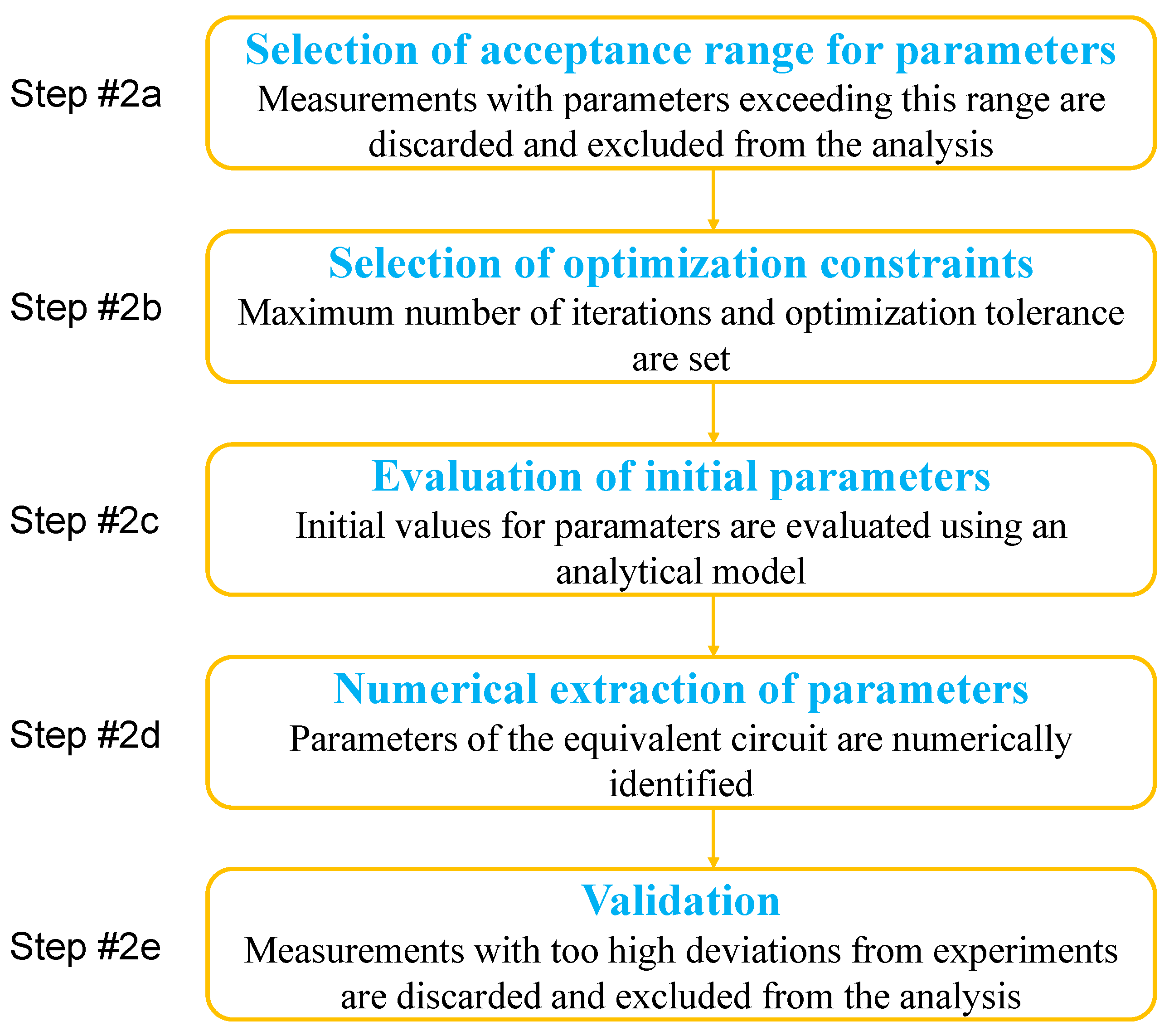
2.2. Step #2—Parameters Extraction

The I-V curve of PV generators can be described by proper equivalent circuits with different parameters. In this step, the five parameters of the single diode model (SDM) [25] are numerically determined using proper algorithms. First, the following acceptance ranges for the five parameters of the SDM are set (Table 1):
Measurements with numerically determined parameters not included in these ranges will be excluded from the analysis.
Then, the main constraints of the adopted algorithms are set. In this case, a cascading combination of the simulated annealing and Nelder–Mead algorithms is used. Indeed, the convergence of the Nelder–Mead algorithm is not guaranteed because its behavior in the neighborhood of local minima of the objective function is not optimal. For this reason, first, the simulated annealing algorithm is applied to identify an initial set of parameters for the Nelder–Mead algorithm sufficiently far from local minima. The suggested constraints for the two algorithms are the following in Table 2:
The initial values for the parameters of the SDM are analytically determined according to the method proposed in Section II of [26]. Then, the parameters are numerically determined with the algorithms by solving the following equation of the SDM:
I = I ph I 0 · ( e q · V j n · k B · T 1 ) ( V + R s I ) R sh
where q is the electron charge (1.6∙10−19 C), kB is the Boltzmann constant (1.38∙10−23 J/K), Vj is the voltage across the terminals of the p-n junction, Iph is the photogenerated current, I0 is the reverse saturation current, n is the diode ideality factor, Rs is the series resistance, and Rsh is the shunt resistance.
Finally, their values are validated. First, it is verified that the obtained parameters are included in the acceptance ranges of step #2a. Then, the I-V curve is traced according to previous equation using the obtained parameters, and the power deviation ∆P at the maximum power point is evaluated. Curves with ∆P > 1% are excluded from the analysis. The flowchart of step #2 is reported in Figure 2.

2.3. Step #3—Nonlinear Regression

As previously mentioned, the equations describing the dependency of each parameter on weather conditions are the following [18]:
I ph = a [ 1 + α ( T c T c , STC ) ] G G STC
where α is the temperature coefficient for short-circuit current (1/K), Tc is PV temperature, Tc,STC is 25 °C, G is solar is solar irradiance (W/m2), GSTC is 1000 W/m2, a is the coefficient to be optimized, which is the photogenerated current at STC.
I 0 = b ( T c T c , STC ) 3 exp ( ( E g , STC T STC E g ( T c ) T c ) 1 k B   )
where Eg(Tc) and Eg,STC are the energy gap of the semiconductor material evaluated at temperature Tc and at STC, respectively. The coefficient b will be optimized, and it corresponds to the reverse saturation current at STC.
n = c + d G + e T c
The behavior of n is not clear in the literature. Thus, a polynomial dependence on G and Tc is supposed by means of coefficients c, d and e. This assumption will be valid according to the results of step #3.
R s = f T c T c , STC ( 1 g log ( G G STC ) )
where g is an adimensional coefficient quantifying the dependence of Rs on G, while the coefficient f is the series resistance at STC.
R sh = h G STC G
where h corresponds to the shunt resistance at STC.
However, [18] does not provide information regarding the green coefficients. In this step, these coefficients are numerically determined and optimized: nonlinear regressions are applied using iterative least squares estimations starting from the parameters determined from the experiments. In particular, the following least squares indicator needs to be minimized:
min i = 1 N ( y i , exp y i , mod ) 2
This indicator evaluates the deviation between the generic parameter from experiments (yi,exp) and the parameter estimated by the model (yi,mod) at the ith couple of weather condition (irradiance and temperature). Its minimization is iterative and permits to identify the optimal coefficients in green.

2.4. Step #4—Power and energy estimation

This step consists of using the optimized equations to evaluate, for each weather condition (irradiance and temperature) from the experimental campaign, the maximum PV power, and the generated energy in the campaign. For each measurement, the corresponding weather conditions are used to estimate the values of the parameters for the SDM according to the optimized equations from previous step. Then, the I-V curves are traced by solving Equation (3), and the maximum power is identified. This value is compared with the experimental data and with the corresponding quantity estimated by the most common model used in the literature, i.e., the Osterwald model (OM) [24]:
P = P STC · G G STC · ( 1 + γ · Δ T )
where PSTC is the rated power in STC, γ is the temperature coefficient for power (provided by the manufacturer), and ∆T = (Tc − 25 °C). Finally, the generated energy is computed by assuming PV power to be constant for an extended time interval (1 min) with respect to the duration of the transient charging of the capacitor (<<1 s at high irradiance). The deviations between the experimental data and the values estimated by the different models are calculated as:
Δ E opt = ( E opt E exp ) E exp
Δ E opt = ( E Ost E exp ) E exp
where Eopt and EOst are the energy values evaluated by the optimized equations and by the OM, respectively, and Eexp is the quantity from experiments.

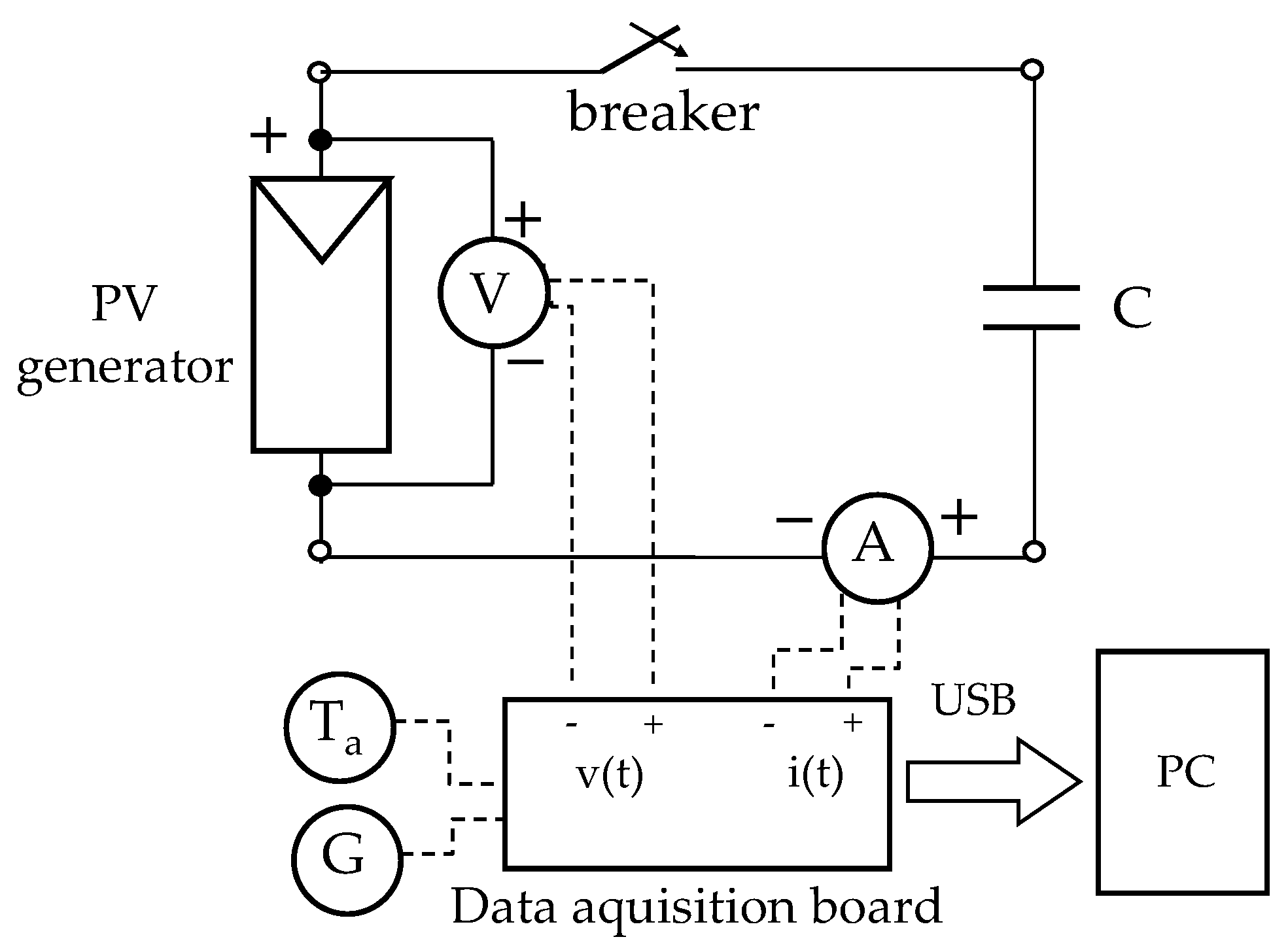
3. Measurement System

Four procedures can be adopted to trace the I-V curve of PV generators and they are based on different principles of operation to control the current provided by the PV module between the short-circuit (V = 0, I = Isc) and the open-circuit state (V = Voc, I = 0) [27]. In particular, they are based on the transient charge of a capacitive load, on a resistive load with variable resistance, on an electronic load, or on a MPPT.
In this work, the first method is used: the PV generator feeds a capacitive load that is initially discharged. In the circuit, a power breaker permits control of the opening and closing of the circuit. When the breaker closes the circuit, the load is fulfilled by the PV generator from short-circuit to open-circuit conditions. A common issue with this method is that current peaks may occur at the beginning of the charging transient, i.e., immediately after the circuit is closed. A common practice is to exclude this first part of the acquired signals from subsequent analyses. However, this operation leads to a loss of information close to the short-circuit point. To solve this issue, a negative pre-charge may be applied to the capacitive load: this procedure permits current peaks when voltage is still negative. As a consequence, the excluded region of the I-V curve is not of interest and the loss of information is avoided. The capacitance of the capacitive load must be properly selected as a function of the desired duration of the charging transient t. Indeed, according to [28], this quantity is a function of the short-circuit current Isc, the open-circuit voltage Voc, the number of parallel-connected PV strings Np, the number of PV modules in series per string Ns (each module consists of Nc series-connected cells), and the capacitance C of the capacitor in the following way:
t = 1.82 · C · N s · V oc N p · I sc
During the measurement of single PV modules, a capacitor with C equal to 10 mF is suggested in order to achieve a transient duration between 0.1 and 0.2 s. In this work, the I-V curves of the PV module are traced using an automatic data acquisition system (ADAS) to store simultaneously the irradiance G, the air temperature Ta, and the current and voltage signals. The acquisition of the I-V curves is performed with a capacitive load, and the duration of its charging transient is < 1 s at each irradiance level. The ADAS is periodically calibrated and it consists of the components listed below [29]:
  • A notebook PC with a LabVIEW software to emulate a digital storage oscilloscope.
  • A multifunction data acquisition board with one A/D converter (successive approximation technology, 16 bit-resolution, sampling rate up to 1.25 MSa/s, maximum input of ±10 V, internal amplifier gains for lower ranges) and multiplexer.
  • A differential voltage probe with two attenuation ratios 20:1 and 200:1 for voltage levels up to 140 V and 1400 V, respectively.
  • Two current probes (Hall effect) with an output sensitivity of 100 mV/A for current values up to ±30 A, one for current measurement and the other one for trigger source.
  • A pyranometer to acquire irradiance with uncertainty < 2%.
  • A thermometer to acquire ambient temperature.
  • A temperature probe to acquire the temperature on the rear side of the module.
  • A capacitive load with capacitance equal to 10 mF.
The schematic of the measurement circuit is presented in Figure 3.

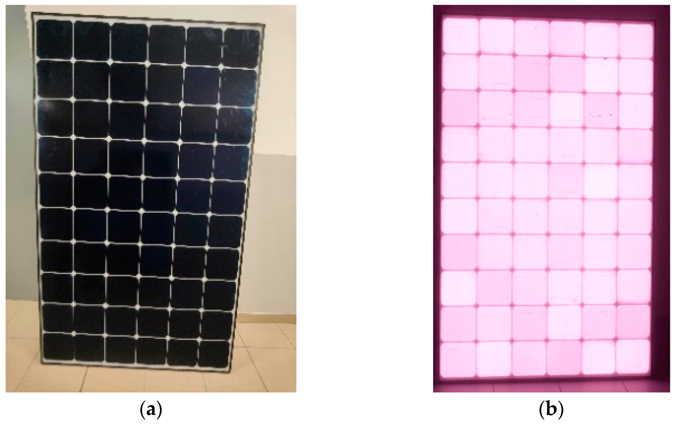
4. PV Module under Test
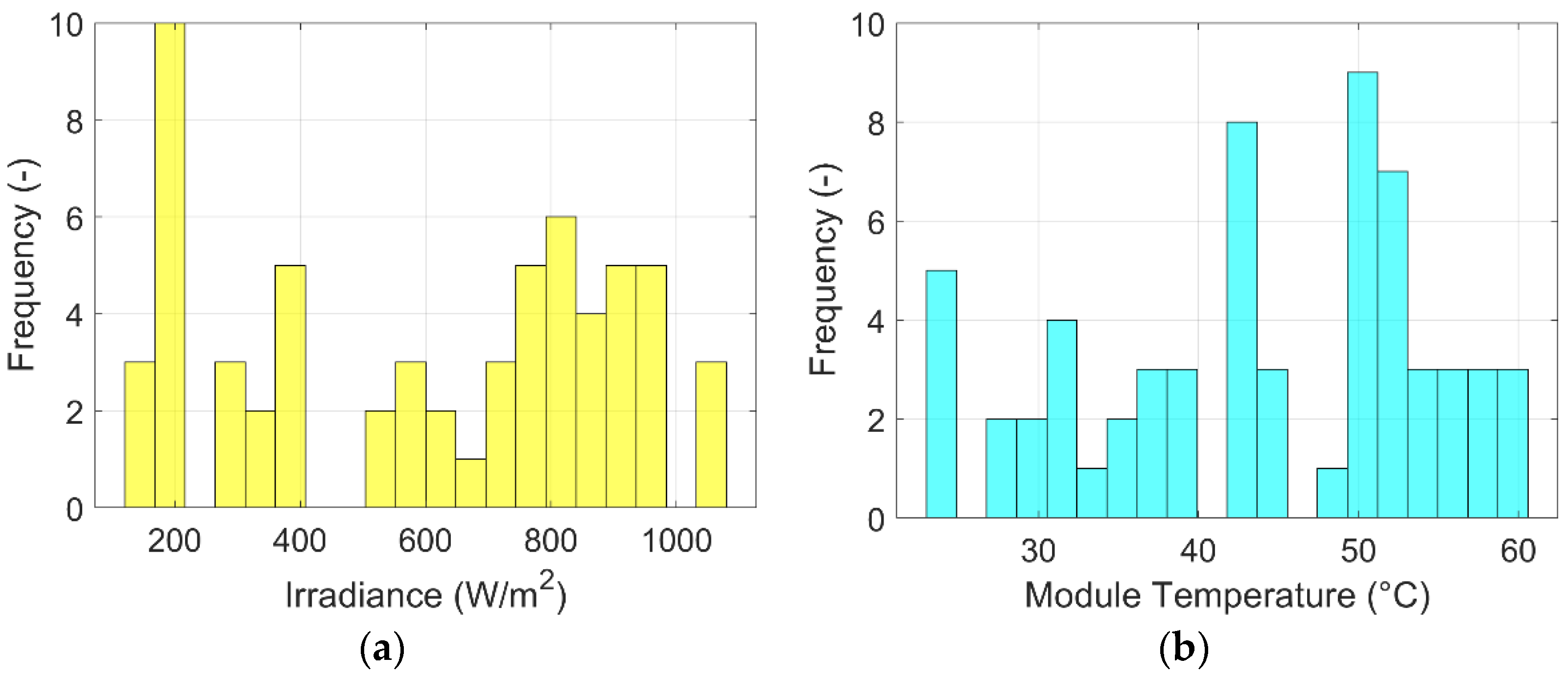
The procedure presented in this work is applied to an all-back contact monocrystalline PV module. The performance of the module was tested before applying the proposed technique: in particular, the I-V curve of the module was determined at standard test conditions (STC) and it was compared with the data provided by the manufacturer. Moreover, an electroluminescence (EL) test [30] was performed to check the presence of defects or mechanical cracks. In particular, the power deviation with respect to manufacturer data is in the uncertainty range of the measurement system, and the EL image in Figure 4 confirms the absence of defects and cracks. According to the manufacturer datasheet, the main electric parameters of the analyzed PV module are summarized in Table 3.

5. Results

The experimental campaign of the module under analysis took place at the Politecnico di Torino (Turin, Italy) in 2021 from March to May, being tested in different weather conditions (62 I-V curves acquired). Figure 5 shows the distribution of the irradiance (yellow bars) and module temperature (blue bars) levels at which the PV performance was measured.
In particular, the irradiance levels range between ≈150 W/m2 and ≈1100 W/m2, while the module temperature is in the range ≈25 °C−≈60 °C. Moreover, the temperature of the module and the wind speed were checked before each test in order to perform the measurements under constant module temperature and in absence of wind. Regarding the numerical extraction of the parameters, a combination of the simulated annealing and the Nelder–Mead algorithms was adopted. Figure 6 shows the distribution of the normalized root mean square error (NRMSE) for the I-V curve and of the error at the maximum power point (MPP). The first quantity estimates the deviation between the experimental data and the curve determined by the parameters of the equivalent circuit, and it is evaluated as follows:
N R M S E = i = 1 N ( I i , mod I i , exp ) 2 N i = 1 N I i ,   exp N 100
where Ii,exp is the current value for the ith point of the I-V curve from experiments, and Ii,mod is the corresponding current value calculated by the model using the parameters of the equivalent circuit. The second parameter is the percentage deviation between the power evaluated at the MPP from experiments and using the parameters.
The numerical extraction was properly performed, obtaining most of NRMSEs < 6∙10−3 and most of the errors at the MPP are in the range −0.5% − +0.5%. The results of step #3 are presented in Figure 7.
The optimized equations (blue curves) and the parameters from experiments (red dots) are presented for each quantity. The optimized coefficients are reported in Table 4.
The effectiveness of the technique is validated by estimating the generated PV power in the measurement conditions. These values (blue curve in Figure 8) are compared with the experiments (green dots) and with the prediction by the OM (red curve). The technique performs better than Osterwald, providing a NRMSE in power prediction of 6.7%. The improvement with respect to the Osterwald error (9.1%) is ≈26%. The energy estimation is performed by assuming constant PV power in a time interval of 1 min. The proposed model underestimates the generated energy (∆Eopt = −0.19%), while the prediction by the OM is overestimated (∆EOst = +8.28%) with respect to the experiments. In a future work, this method will be applied to wider experimental datasets. Figure 9 presents the irradiance and air temperature distribution for a reference year in Turin (hourly updated, for a PV installation with azimuth = 0° and tilt angle = 30°) during sunlight hours.
According to Figure 8, the Osterwald model performs better in the irradiance range ≈600–≈800 W/m2: however, according to Figure 9, most of irradiance levels (≈86%) are not included in this range. Thus, the proposed model is expected to outperform the Osterwald model with wider datasets as well.

6. Conclusions

For a PV generator, the knowledge of its equivalent parameters is fundamental to deeply study and simulate its operation in any weather condition. In the literature, many papers propose methods to extract these parameters from measurements. However, generally, they refer to specific weather conditions, and their dependence on irradiance and temperature is not investigated. Moreover, a few papers present some equations describing the dependence of each parameter on weather conditions, but some of their coefficients are unknown. As a consequence, this information cannot be used to predict the PV energy in any weather condition. This work proposes an innovative technique to assess the generated energy by PV modules starting from the knowledge of their equivalent parameters. The model is applied to a highly efficient PV generator with all-back contact, monocrystalline silicon technology, and rated power of 370 W. An experimental campaign was carried out for this module at Politecnico di Torino (Turin, Italy) in three months of 2021. The module was tested under a wide range of irradiance (width of 850 W/m2) and module temperature (35 °C width of the range). Starting from the equations known in the literature to describe the dependency of each parameter on weather condition, experimental data were used to optimize the values of their coefficients. The PV power generated during the experimental campaign was estimated according to these optimized equations and with the Osterwald model. The deviations with respect to the experiments are quantified by evaluating the corresponding NRMSE for power estimation and estimating the energy deviations from experimental data. The results show that the optimized equations outperform the Osterwald model, reducing the NRMSE on power prediction by ≈26%. Moreover, regarding energy prediction, the error by the model (−0.19%) is noticeably lower than Osterwald (+8.28%). In the future, this method will be applied to wider experimental datasets, and is expected to outperform the Osterwald model in this condition as well. Finally, in future works, more PV modules will be tested, and the risk of overfitting will be minimized by proposing different sets of coefficients for different groups of PV modules. The classification of the modules will be performed according to some criteria (for example, according to the manufacturing date, the rated power, the position of the electrical contacts or other properties).

Author Contributions

Conceptualization, F.S. and G.M.; methodology, F.S. and G.M.; software, G.M. and H.S.; validation, G.M., H.S. and M.A.E.Q.; formal analysis, G.M. and H.S.; investigation, G.M. and A.A.; resources, G.M., H.S. and M.A.E.Q.; data curation, G.M. and H.S.; writing—original draft preparation, G.M. and M.A.E.Q.; writing—review and editing, G.M. and A.A.; visualization, G.M. and A.A.; supervision, F.S. and A.C.; All authors have read and agreed to the published version of the manuscript.

Funding

This research received no external funding.

Institutional Review Board Statement

Not applicable.

Informed Consent Statement

Not applicable.

Data Availability Statement

Not available.

Conflicts of Interest

The authors declare no conflict of interest.

References

  1. Di Leo, P.; Spertino, F.; Fichera, S.; Malgaroli, G.; Ratclif, A. Improvement of Self-Sufficiency for an Innovative Nearly Zero Energy Building by Photovoltaic Generators. In Proceedings of the 2019 IEEE Milan PowerTech, Milan, Italy, 23–27 June 2019. [Google Scholar]
  2. Ciocia, A.; Amato, A.; Di Leo, P.; Fichera, S.; Malgaroli, G.; Spertino, F.; Tzanova, S. Self-Consumption and Self-Sufficiency in Photovoltaic Systems: Effect of Grid Limitation and Storage Installation. Energies 2021, 14, 1591. [Google Scholar] [CrossRef]
  3. Spertino, F.; Fichera, S.; Ciocia, A.; Malgaroli, G.; Di Leo, P.; Ratclif, A. Toward the Complete Self-Sufficiency of an NZEBS Microgrid by Photovoltaic Generators and Heat Pumps: Methods and Applications. IEEE Trans. Ind. Appl. 2019, 55, 7028–7040. [Google Scholar] [CrossRef]
  4. Bahrami, M.; Gavagsaz-Ghoachani, R.; Zandi, M.; Phattanasak, M.; Maranzana, G.; Nahid-Mobarakeh, B.; Pierfederici, S.; Meibody-Tabar, F. Hybrid Maximum Power Point Tracking Algorithm with Improved Dynamic Performance. Renew. Energy 2019, 130, 982–991. [Google Scholar] [CrossRef]
  5. Harrag, A.; Messalti, S. Extraction of Solar Cell Parameters Using Genetic Algorithm. In Proceedings of the 2015 4th International Conference on Electrical Engineering (ICEE), Boumerdes, Algeria, 13–15 December 2015. [Google Scholar]
  6. Spertino, F.; Ciocia, A.; Di Leo, P.; Tommasini, R.; Berardone, I.; Corrado, M.; Infuso, A.; Paggi, M. A Power and Energy Procedure in Operating Photovoltaic Systems to Quantify the Losses According to the Causes. Sol. Energy 2015, 118, 313–326. [Google Scholar] [CrossRef] [Green Version]
  7. Lappalainen, K.; Valkealahti, S. Effects of PV Array Layout, Electrical Configuration and Geographic Orientation on Mismatch Losses Caused by Moving Clouds. Sol. Energy 2017, 144, 548–555. [Google Scholar] [CrossRef]
  8. Mohapatra, A.; Nayak, B.; Das, P.; Mohanty, K.B. A Review on MPPT Techniques of PV System under Partial Shading Condition. Renew. Sustain. Energy Rev. 2017, 80, 854–867. [Google Scholar] [CrossRef]
  9. Ahmad, J.; Spertino, F.; Ciocia, A.; Di Leo, P. A Maximum Power Point Tracker for Module Integrated PV Systems under Rapidly Changing Irradiance Conditions. In Proceedings of the 2015 International Conference on Smart Grid and Clean Energy Technologies (ICSGCE), Offenburg, Germany, 20–23 October 2015. [Google Scholar]
  10. Bizzarri, F.; Nitti, S.; Malgaroli, G. The Use of Drones in the Maintenance of Photovoltaic Fields. In Proceedings of the E3S Web of Conferences, Torino, Italy, 12–16 November 2018; Volume 119. [Google Scholar] [CrossRef]
  11. Kebir, S.T.; Haddadi, M.; Ait-Cheikh, M.S. An Overview of Solar Cells Parameters Extraction Methods. In Proceedings of the 3rd International Conference on Control, Engineering and Information Technology (CEIT), Tlemcen, Algeria, 25–27 May 2015. [Google Scholar]
  12. Nassar-Eddine, I.; Obbadi, A.; Errami, Y.; el Fajri, A.; Agunaou, M. Parameter Estimation of Photovoltaic Modules Using Iterative Method and the Lambert W Function: A Comparative Study. Energy Convers. Manag. 2016, 119, 37–48. [Google Scholar] [CrossRef]
  13. Awadallah, M.A.; Venkatesh, B. Estimation of PV Module Parameters from Datasheet Information Using Optimization Techniques. In Proceedings of the 2015 IEEE International Conference on Industrial Technology (ICIT), Seville, Spain, 17–19 March 2015. [Google Scholar]
  14. Rhouma, M.B.H.; Gastli, A. An Extraction Method for the Parameters of the Solar Cell Single-Diode-Model. In Proceedings of the 2018 2nd European Conference on Electrical Engineering and Computer Science (EECS), Bern, Switzerland, 20–22 December 2018. [Google Scholar]
  15. Ishaque, K.; Salam, Z.; Taheri, H.; Shamsudin, A. Parameter Extraction of Photovoltaic Cell Using Differential Evolution Method. In Proceedings of the 2011 IEEE Applied Power Electronics Colloquium (IAPEC), Johor Bahru, Malaysia, 18–19 April 2011. [Google Scholar]
  16. Muhsen, D.H.; Ghazali, A.B.; Khatib, T.; Abed, I.A. A Comparative Study of Evolutionary Algorithms and Adapting Control Parameters for Estimating the Parameters of a Single-Diode Photovoltaic Module’s Model. Renew. Energy 2016, 96, 377–389. [Google Scholar] [CrossRef]
  17. Khare, A.; Rangnekar, S. A Review of Particle Swarm Optimization and Its Applications in Solar Photovoltaic System. Appl. Soft Comput. J. 2013, 13, 2997–3006. [Google Scholar] [CrossRef]
  18. Tossa, A.K.; Soro, Y.M.; Azoumah, Y.; Yamegueu, D. A New Approach to Estimate the Performance and Energy Productivity of Photovoltaic Modules in Real Operating Conditions. Sol. Energy 2014, 110, 543–560. [Google Scholar] [CrossRef]
  19. Jadli, U.; Thakur, P.; Shukla, R.D. A New Parameter Estimation Method of Solar Photovoltaic. IEEE J. Photovolt. 2018, 8, 239–247. [Google Scholar] [CrossRef]
  20. Oudira, H.; Mezache, A.; Chouder, A. Solar Cell Parameters Extraction of Photovoltaic Module Using NeIder-Mead Optimization. In Proceedings of the 2018 IEEE 5th International Congress on Information Science and Technology (CiSt), Marrakech, Morocco, 21–27 October 2018. [Google Scholar]
  21. Reza, M.N.; Mominuzzaman, S.M. Extraction of Equivalent Circuit Parameters for CNT Incorporated Perovskite Solar Cells Using Newton-Raphson Method. In Proceedings of the 2018 10th International Conference on Electrical and Computer Engineering (ICECE), Dhaka, Bangladesh, 20–22 December 2018. [Google Scholar]
  22. Kumar, M.; Shiva Krishna Rao, K.D. Modelling and Parameter Estimation of Solar Cell Using Genetic Algorithm. In Proceedings of the 2019 International Conference on Intelligent Computing and Control Systems (ICCS), Madurai, India, 15–17 May 2019. [Google Scholar]
  23. Merchaoui, M.; Sakly, A.; Mimouni, M.F. Particle Swarm Optimisation with Adaptive Mutation Strategy for Photovoltaic Solar Cell/Module Parameter Extraction. Energy Convers. Manag. 2018, 175, 151–163. [Google Scholar] [CrossRef]
  24. Campanelli, M.B.; Osterwald, C.R. Effective Irradiance Ratios to Improve I-V Curve Measurements and Diode Modeling over a Range of Temperature and Spectral and Total Irradiance. IEEE J. Photovolt. 2016, 6, 48–55. [Google Scholar] [CrossRef]
  25. Humada, A.M.; Hojabri, M.; Mekhilef, S.; Hamada, H.M. Solar Cell Parameters Extraction Based on Single and Double-Diode Models: A Review. Renew. Sustain. Energy Rev. 2016, 56, 494–509. [Google Scholar] [CrossRef] [Green Version]
  26. Majdoul, R.; Abdelmounim, E.; Aboulfatah, M.; Touati, A.W.; Moutabir, A.; Abouloifa, A. Combined Analytical and Numerical Approach to Determine the Four Parameters of the Photovoltaic Cells Models. In Proceedings of the 2015 International Conference on Electrical and Information Technologies (ICEIT), Marrakech, Morocco, 25–27 March 2015. [Google Scholar]
  27. Duran, E.; Piliougine, M.; Sidrach-De-Cardona, M.; Galan, J.; Andujar, J.M. Different Methods to Obtain the I-V Curve of PV Modules: A Review. In Proceedings of the Conference Record of the IEEE Photovoltaic Specialists Conference, San Diego, CA, USA, 11–16 May 2008. [Google Scholar]
  28. Spertino, F.; Ahmad, J.; Ciocia, A.; Di Leo, P.; Murtaza, A.F.; Chiaberge, M. Capacitor Charging Method for I–V Curve Tracer and MPPT in Photovoltaic Systems. Sol. Energy 2015, 119, 461–473. [Google Scholar] [CrossRef] [Green Version]
  29. Ciocia, A.; Di Leo, P.; Fichera, S.; Giordano, F.; Malgaroli, G.; Spertino, F. A Novel Procedure to Adjust the Equivalent Circuit Parameters of Photovoltaic Modules under Shading. In Proceedings of the 2020 International Symposium on Power Electronics, Electrical Drives, Automation and Motion (SPEEDAM), Sorrento, Italy,, 24–26 June 2020. [Google Scholar]
  30. Ciocia, A.; Carullo, A.; Di Leo, P.; Malgaroli, G.; Spertino, F. Realization and Use of an IR Camera for Laboratory and On-Field Electroluminescence Inspections of Silicon Photovoltaic Modules. In Proceedings of the 2019 IEEE 46th Photovoltaic Specialists Conference (PVSC), Chicago, IL, USA, 16–21 June 2019. [Google Scholar]
Figure 1. Flowchart of the methodology.
Solar 02 00018 g001
Figure 2. Flowchart of step #2.
Solar 02 00018 g002
Figure 3. Schematic of the measurement circuit.
Solar 02 00018 g003
Figure 4. PV module under test in visible light (a) and during the EL test (b).
Solar 02 00018 g004
Figure 5. Irradiance (a) and module temperature (b) distribution.
Solar 02 00018 g005
Figure 6. Distribution of NRMSE for the I-V curve (a) and of the error at the MPP (b).
Solar 02 00018 g006
Figure 7. Parameters of the equivalent circuit as functions of G and Tc: Iph (a), I0 (b), n (c,d), Rs (e,f), and Rsh (g).
Solar 02 00018 g007aSolar 02 00018 g007b
Figure 8. Power prediction from the technique and OM vs. experiments.
Solar 02 00018 g008
Figure 9. Irradiance (a) and air temperature (b) distribution (reference year in Turin).
Solar 02 00018 g009
Table 1. Suggested acceptance ranges for the parameters of the SDM.
ParameterRange
Iph0–15 A
I00–10−3 A
n0–4
Rs0–1 Ω
Rsh0–20,000 Ω
Table 2. Suggested constraints for the SA/NM algorithms.
Tolerance10−30
Maximum number of iterations10,000
Table 3. Electrical parameters of PV module from manufacturer datasheet.
Rated power PPV370 W
Short-circuit current Isc10.82 A
Open-circuit voltage Voc42.8 V
Current temperature coefficient α0.04%/°C
Voltage temperature coefficient β−0.24%/°C
Power temperature coefficient γ−0.3%/°C
Nominal Operating Cell Temperature NOCT44 °C
Number of cells in series Nc60
Table 4. Coefficients of the optimized equations.
a10.47 A
b4.17∙10−8 A
c2.48
d7.37∙10−4 m2/W
e−4.62∙10−3 1/K
f0.0037 Ω
g17.19
h112.1 Ω
Publisher’s Note: MDPI stays neutral with regard to jurisdictional claims in published maps and institutional affiliations.

