Article

Recurringly Hypoxic: Bottom Water Oxygen Depletion Is Linked to Temperature and Precipitation in a Great Lakes Estuary

1
Annis Water Resources Institute, Grand Valley State University, Muskegon, MI 49441, USA
2
School for Environment and Sustainability, University of Michigan, Ann Arbor, MI 48109, USA
*
Author to whom correspondence should be addressed.
Hydrobiology 2023, 2(2), 410-430; https://doi.org/10.3390/hydrobiology2020027
Submission received: 8 April 2023 / Revised: 23 May 2023 / Accepted: 30 May 2023 / Published: 17 June 2023
(This article belongs to the Special Issue Feature Papers in Hydrobiology 2022–2023)

Abstract

:
Hypolimnetic hypoxia is expanding globally due to anthropogenic eutrophication and climate warming. Muskegon Lake, a Great Lakes estuary, experiences annually recurring hypoxia, impairing ecological, social, and economic benefits. Using high-frequency, time-series Muskegon Lake Observatory (MLO) data, we quantified the dynamics of hypoxia and developed a hypoxia severity index to estimate the spatiotemporal extent of hypoxia during 2011–2021. We also analyzed United States Geological Survey’s temperature and discharge data on the Muskegon River to explain the annual variability in the hypoxia severity index. Severe hypoxia occurred in warmer years with greater stratification, fewer wind mixing events, warmer winter river temperatures, and less winter and spring precipitation, as in 2012 and 2021. Conversely, milder hypoxia was prevalent in colder years with a later stratification onset, more mixing events, colder river temperatures, and more winter and spring precipitation, as in 2015 and 2019. Thus, knowledge of environmental conditions prior to the onset of stratification may be useful for predicting the potential severity of hypoxia for any year. While consistent multi-year trends in hypoxia were not discernible, our findings suggest that temperature and precipitation are major drivers of hypoxia and that as surface waters warm, it will lead to the further deoxygenation of Earth’s inland waters.

1. Introduction

The bottom waters of marine and freshwater ecosystems are increasingly experiencing hypoxic conditions due to increased eutrophication and climate change [1,2,3,4,5]. Hypoxia is defined as an aquatic ecosystem experiencing dissolved oxygen (DO) at or below 2 mg/L [5,6]. Hypoxia is categorized with this concentration because of the lethal and sub-lethal effects on living organisms corresponding with this threshold, including but not limited to fish kills and deterring fish from inhabiting bottom waters [7,8]. Within this study, we explore the more common <2 mg/L definition of severe hypoxia. DO between 4 mg/L and 2 mg/L is defined as mild hypoxia because sensitive aquatic species within Muskegon Lake, such as the endangered Acipenser fulvescens (Lake Sturgeon), are unable to withstand either threshold, while more resilient species can withstand mild hypoxia [7]. Hypoxia in freshwater and marine ecosystems occurs in four known ways: diel hypoxia, hypolimnetic hypoxia, overwinter hypoxia, and episodic hypoxia [9]. In the present study, hypolimnetic hypoxia will be the sole focus. As climate change and extensive eutrophication continue to intensify, monitoring and understanding trends in hypoxic zones is needed to reduce the negative impacts inflicted upon freshwater and marine ecosystems globally.
The Laurentian Great Lakes basin is the largest contiguous body of freshwater, with ~19% of the liquid freshwater on Earth’s surface, and also a hotspot for hypoxia. Across the Great Lakes region, approximately 20 lakes and estuaries are known to experience hypoxia on a yearly basis [9], including major bodies of water such as Lake Erie, Green Bay, Saginaw Bay, Hamilton Harbour, and Muskegon Lake [10,11,12]. Muskegon Lake, a drowned river mouth Great Lakes estuary that connects the Muskegon River to Lake Michigan, is a dynamic lotic and lentic ecosystem that aquatic and terrestrial species need for survival (Figure 1) [13,14]. Muskegon Lake was initially listed as a Great Lakes Area of Concern (AOC) due to past industrial and agricultural contamination and eutrophication. Restoration and continued research efforts intend to remove Muskegon Lake from its current status as an AOC [15]. At the time of writing, beneficial use impairments that still persist include eutrophication, degradation of benthos, degradation of fish populations, and loss of fish habitat—all of which may be associated with hypoxia in the hypolimnion.
The effects of climate change within the Great Lakes region are major contributors to future hypoxia. Global and regional climate projections of increased air temperature and precipitation patterns suggest that these conditions will play major roles in shaping the future of aquatic ecosystems in the Great Lakes region [4,16,17,18,19,20]. Byun and Hamlet (2018) projected that midwestern U.S. and Great Lakes temperatures will continue to rise with overall increases in air temperature up to 6.5 °C by 2100 under the Representative Concentration Pathway (RCP) 8.5 emissions scenario. Alternatively, under the RCP 4.5 emissions scenario, the temperature increase is projected to be around 3.3 °C by the same year. Moreover, there is an estimated 30% increase in precipitation during the winter and spring seasons, while a 15% decrease in precipitation is anticipated during the summer by the year 2080. The frequency of heat waves across the conterminous United States has more than doubled, from 11 heatwave days in 1996 to 25 heatwave days in 2021. This exposes freshwater organisms to the limits of their physiologic tolerance and endangers the stability of aquatic ecosystems [21]. Furthermore, hypoxia—fueled by eutrophication and facilitated by warming—is often coincident with increased acidity in aquatic ecosystems, where the interactive effects of decreased oxygen and increased acidity may alter food webs [22]. Water temperatures within the Great Lakes basin are expected to respond faster than air temperatures to climate change due to positive ice-albedo feedback [23]. In Lake Superior, surface water temperatures increased more rapidly than local air temperatures due to decreased ice coverage and an earlier onset of stratification [23]. Although surface water temperatures are responding quicker to climate change, air temperatures and surface water temperatures are seasonally correlated in warming trends [24]. As climate change continues to shape Great Lakes regional air temperatures and precipitation, hypoxia dynamics may ultimately vary in concert [19].
Another contributor to hypoxia is eutrophication, which is the symptom of excess nutrient input into an aquatic ecosystem leading to abnormally high productivity. Eutrophication is often caused by runoff from agricultural and industrial pollutants such as fertilizers and industrial waste. As eutrophication impairs vulnerable freshwater ecosystems, phytoplankton grow and then die off, sinking into the hypolimnion and resulting in more organic matter to be decomposed, increasing oxygen consumption [25,26,27]. Within Muskegon Lake, nutrients that enter the system are well retained within the lake, creating current eutrophic conditions from re-suspended past nutrient loads [28]. Eutrophication not only affects ecological functions within a body of water but also affects economic and cultural functions such as the uptake of drinking water and recreational activities [29,30,31]. Lakes with low algal community stability are often overtaken by cyanobacteria species, unlike ecosystems with high algal community stability, which are dominated by diatoms and green algae [32]. Due to the projected increases in precipitation and temperature in the Great Lakes region, cyanobacterial blooms will likely continue to thrive under conditions of decreased phytoplankton stability and increased water column stratification that may generate intensified hypoxia.
For the reasons stated above, Muskegon Lake presents a model Great Lakes habitat for studies of hypoxia dynamics that could serve as a Great Lakes sentinel for future hypoxic conditions within the region (Figure 1) [33]. The objectives of this study were to (1) quantify the temporal characteristics of hypoxia throughout a decade-long high-frequency time-series dataset of hypoxia, (2) identify the environmental and meteorological conditions that separate severe and mild hypoxic years, and (3) predict the future of hypoxia within Muskegon Lake based on temporal trends. By critically analyzing the high-frequency Muskegon Lake Observatory (MLO) environmental data, our research investigates the trends of hypolimnetic hypoxia in Muskegon Lake across years of varying air temperatures, surface water temperatures, and precipitation.

2. Materials and Methods
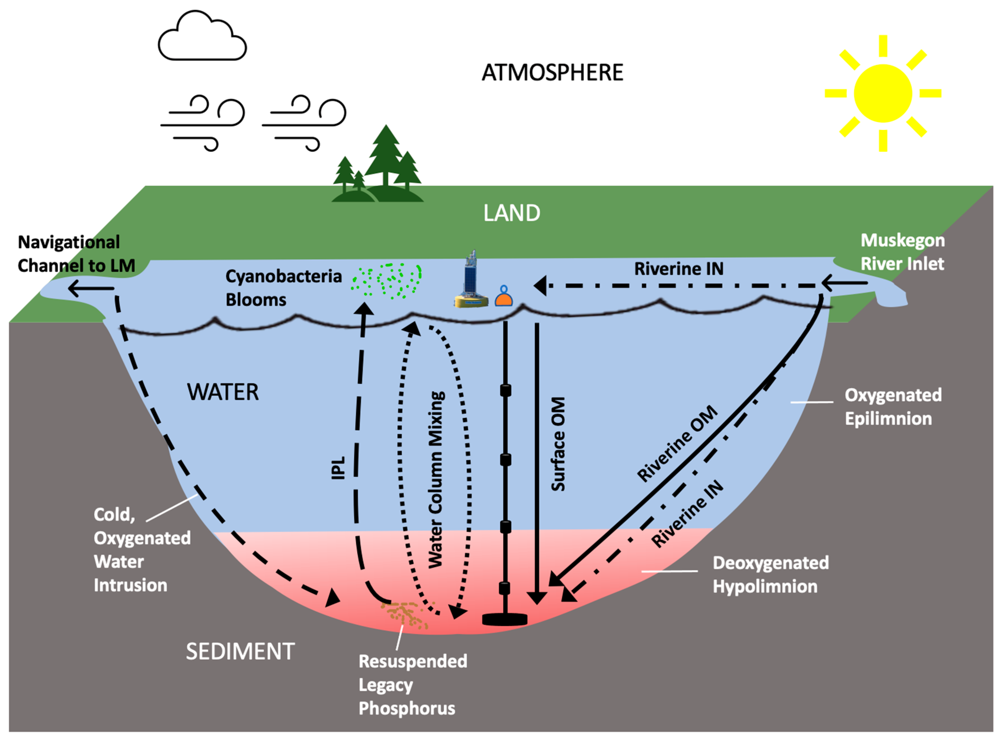
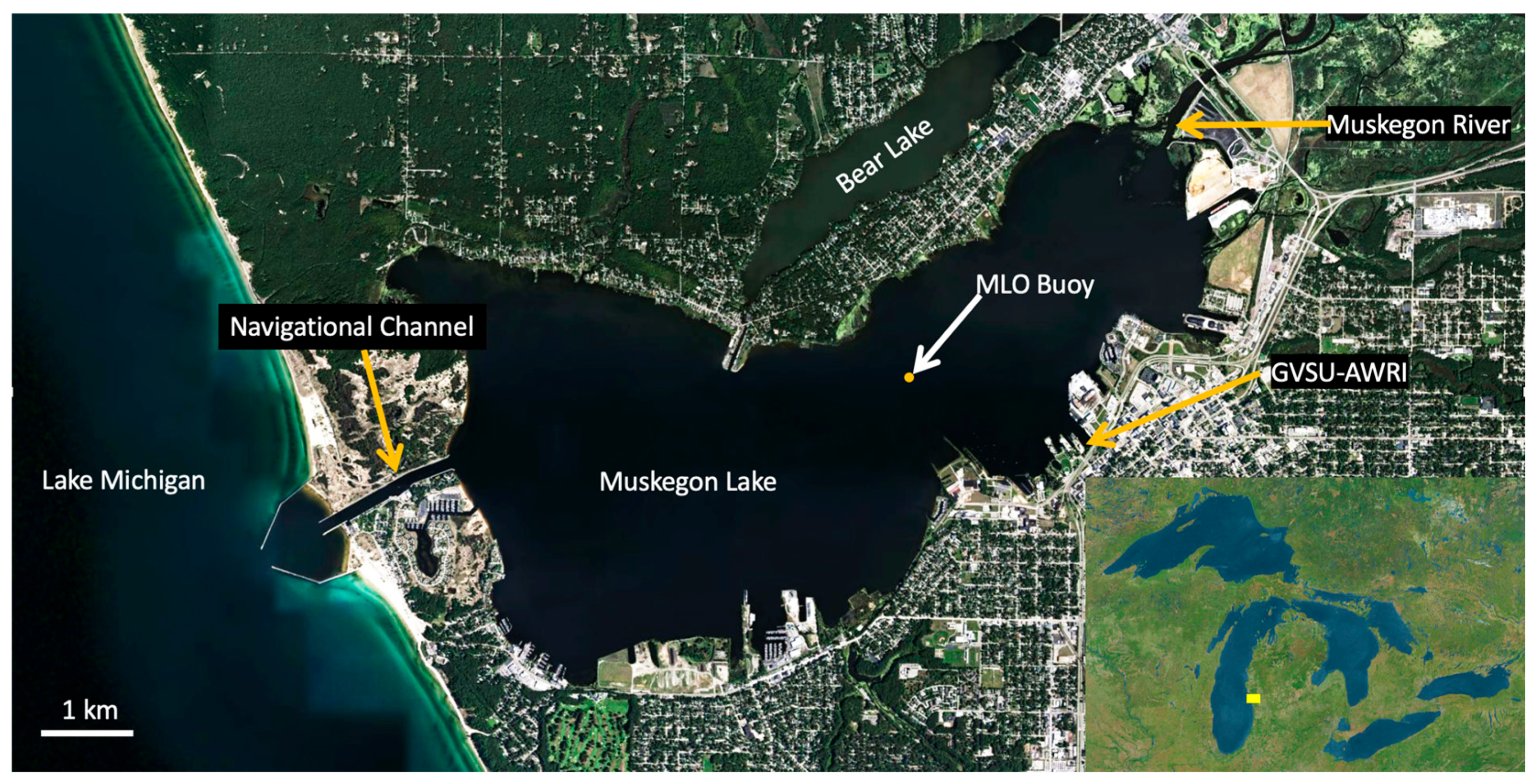
2.1. Study Site

Muskegon Lake (43.23° N, 86.29° W), located in Muskegon, Michigan, USA, is a mesotrophic drowned river mouth Great Lakes estuary (Figure 2). The Muskegon River watershed is the second largest in the state of Michigan, and land use within the Muskegon Lake watershed is predominantly forested (53.2%) and agricultural (23%), with a relatively small but increasing number of urban areas (4.2%) [34]. The estuary has three inflows, including the Muskegon River, Bear Lake, and Ruddiman Creek, with the Muskegon River contributing the most inflow by a considerable margin. A singular outflow through a navigation channel on the west end of the lake drains Muskegon Lake into Lake Michigan. Muskegon Lake has a surface area of 17 km2 and a water volume of 119 million m3. The estuary has an average hydraulic residence time of 23 days, a mean water depth of 7 m, and a maximum water depth of 21 m [35]. Secchi disc depth averaged 2.3 m in Muskegon Lake during the study period, implying that depths below 8 m were consistently aphotic. Muskegon Lake is a Great Lakes Area of Concern (AOC), and continued research and restoration are needed to free the ecosystem from its industrial waste-ridden past [15].

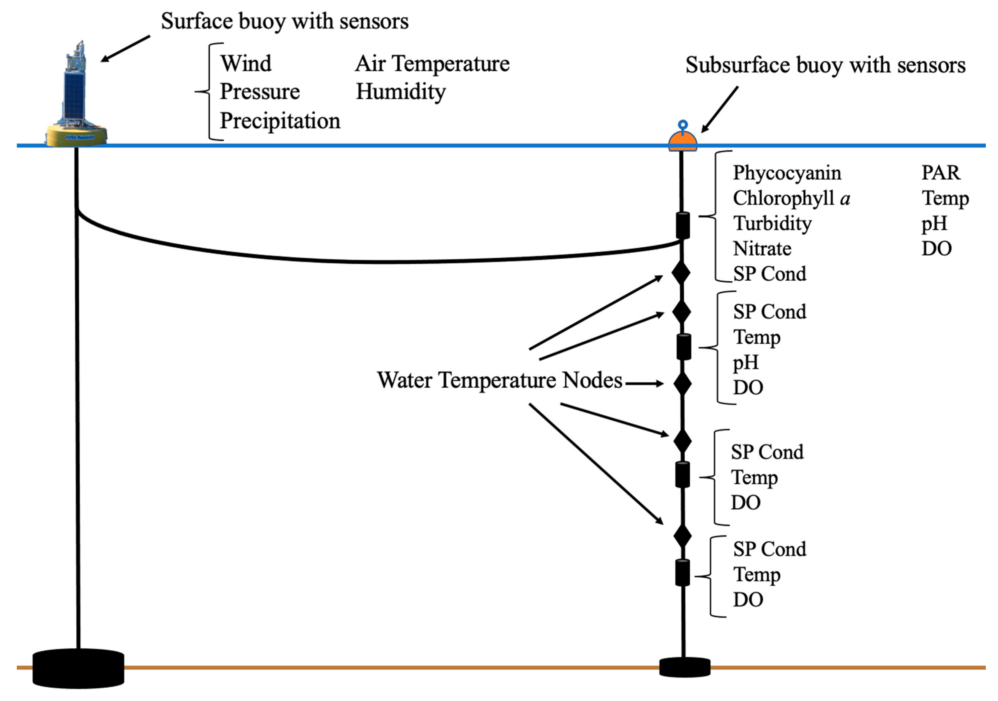
2.2. Muskegon Lake Observatory Data Collection

The Muskegon Lake Observatory (MLO; www.gvsu.edu/buoy, accessed on 30 October 2022) is a high-frequency time-series observatory buoy managed by the Biddanda Lab at the Annis Water Resources Institute (GVSU-AWRI, Muskegon, MI, USA; Figure S1). The buoy is routinely deployed in the bathymetric and hydrographic centers of Muskegon Lake. Since 2011, the MLO has provided meteorological and water quality data for local recreationalists, researchers, teachers, and professors [36]. Sitting atop the buoy, the meteorological station measures wind speed, direction, precipitation, air temperature, humidity, and barometric pressure. The MLO is outfitted with YSI (Yellow Springs Instruments) 6600/6920 sondes at depths of 2, 5, 8, and 11 m, a Turner Designs C3 submersible fluorometer at 2 m, a Satlantic submersible ultraviolet nitrate analyzer at 2 m, a LI-COR photosynthetically active radiation sensor at 2 m, and NEXENS temperature nodes at 2, 4, 6, 8, 10, and 11 m (Figure 3). The water quality parameters measured by these sondes and sensors are chlorophyll a, phycocyanin, dissolved oxygen (DO), and water temperature. All sensors were calibrated before the MLO was deployed each spring. A quality assurance calibration (dirty sensor check) was performed upon the retrieval of the MLO in the fall after every year to ensure the quality of the data throughout the year. Water quality data and meteorological data are acquired every 15 min and every 5 min, respectively. The data utilized in this study are daily averages of the parameters. Missing data occur variably in the data sets due to times of maintenance, servicing of the buoy, and heavy biofouling.

2.3. Data Visualization and Calculations

Stratification and hypoxia in the water column were visualized with DO and water temperature heat maps from 2011–2021. Heat maps were created using daily averaged water temperatures and DO concentrations at 2, 4, 6, 8, 10, and 11 m and 2, 5, 8, and 11 m, respectively. Due to the MLO’s central location, MLO data observed in the heat maps can be used as a proxy to understand hypoxia dynamics throughout Muskegon Lake as a whole [10,37]. Each heat map was scaled to the dates of the earliest MLO deployment and the latest MLO retrieval throughout the decade. The temperature scale incorporated the highest and lowest water temperatures throughout the decade and was synchronized among every heat map. The R package RLakeAnalyzer was used to create the heat maps in RStudio Version 2021 [38]. RLakeAnalyzer interpolates between the depths of the MLO heat maps by discretely calculating the vertical density gradient between the upper and lower sensors [39].
Observing the spatial and temporal extent of MLO water temperature and DO in the heat maps between years provides an overview of hypoxia dynamics on a year-to-year basis. Time-series graphs of air temperature, surface temperature, Schmidt stability, surface chlorophyll-a concentrations, and DO were included to examine their effects on the severity of hypoxia throughout the decade. A histogram of DO below the near anoxia threshold throughout the decade with bins of 0.1 mg/L was drawn to determine which years were most likely anoxic and the duration of anoxia. By utilizing daily averages, it is almost impossible for these averages to equal complete anoxia (0.0 mg/L). Therefore, the histogram analyzes the exact breakdown of near anoxia (<1.0 mg/L) between years to determine the most anoxic years.

2.4. Hypoxic Severity Index

Comparisons of hypoxia across years were determined by the count and DO concentration of mild and severe hypoxic days during a given year through our newly developed hypoxia severity index. Previously developed methods, such as the Hypoxic Factor [40], which evaluates hypoxia on a temporal and spatial basis, and Hypolimnetic Oxygen Demand [41,42], which evaluates hypoxia based on hypolimnetic oxygen decreases at the beginning of seasonal hypoxia, do not consider both duration and severity of hypoxia in one metric such as the hypoxia severity index. Within the present study, the ability to measure the variable severity quickly and easily across years could reveal a change in hypoxia in this ecosystem due to increasing climate change and anthropogenic inputs. Therefore, an index was created to compare hypoxia from one year to another via the following formula, in which mild hypoxia in this study was classified as 4.0 > 2.0 mg/L and severe hypoxia was classified as 2.0 mg/L ≥ 0.0 mg/L:
Hypoxia Severity Index = ((#Severe hypoxic days ×1.5) + #Mild hypoxic days)/Avg. DO of hypoxic days
For instance, if three total days of hypoxia occurred with DO concentrations of 2.0, 1.5, and 1.0, the average DO of hypoxic days would be 1.5. Days of severe hypoxia are weighted by 1.5 to raise the influence of severe hypoxic days due to their greater ecological impact in relation to mild hypoxia in Muskegon Lake [7,43]. A mildly hypoxic year was categorized as one with a shortened stratification period in the water column that coincided with a shorter duration of hypoxia. A severely hypoxic year was categorized as one with a longer stratification period that coincided with a prolonged duration of hypoxia. A sensitivity test was conducted to examine the sensitivity of the three variables to influencing the hypoxic severity index. Linear regression and Pearson correlation were conducted to determine a trend in severity over the study period.
A multiple linear regression analysis was performed to determine which environmental variables induced severe hypoxia. Data was collected from the United States Geological Survey (USGS) gage at the Croton Dam on the Muskegon River [44]. We utilized linear regressions of discharge and temperature at the Croton Dam to free-flowing locations of the Muskegon River, such as the upstream USGS gages in Evart and Big Rapids, Michigan, and determined that the Croton Dam USGS gage provided a reliable representation of the integrated precipitation, discharge, and temperature across the entire Muskegon River watershed from January to July—before the onset of hypoxia. The regression included Muskegon Lake’s daily averaged surface temperature, precipitation, and Schmidt stability recorded by the MLO and Muskegon River discharge and temperature (Table S1). To further examine the correlation between the severity of hypoxia and environmental parameters, a principal component analysis (PCA) was conducted. In the PCA, the hypoxia severity index was compared to monthly averaged phycocyanin, chlorophyll a, Schmidt stability, and surface temperature from June to October to incorporate the entire hypoxic season.

2.5. Schmidt Stability
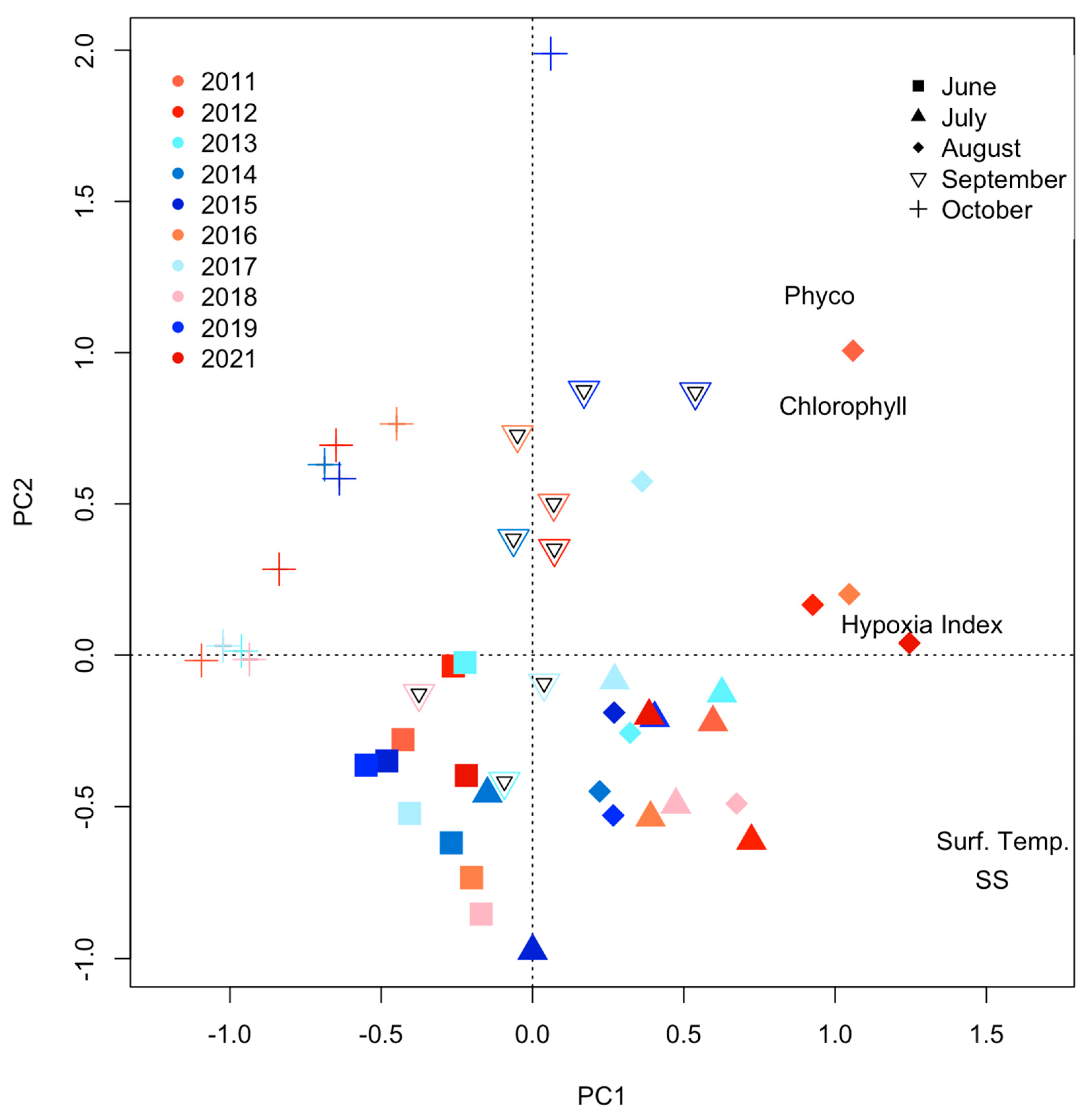
Schmidt stability was calculated utilizing daily averaged water temperature data from 2011 to 2021 [38]. Schmidt stability is an estimated measure of the amount of energy it would take to mix the entire water column evenly. Coefficients of Schmidt stability were calculated from May to September, which included the onset and breakdown of stratification in Muskegon Lake, and compared across years to determine which years endured stronger stratification compared to other years with weaker stratification [45]. Time series graphs were created to visualize the temporal trends of the Schmidt stability coefficients. The R package RLakeAnalyzer was used to generate the Schmidt stability coefficients in RStudio Version 2021 [46,47,48,49].

3. Results

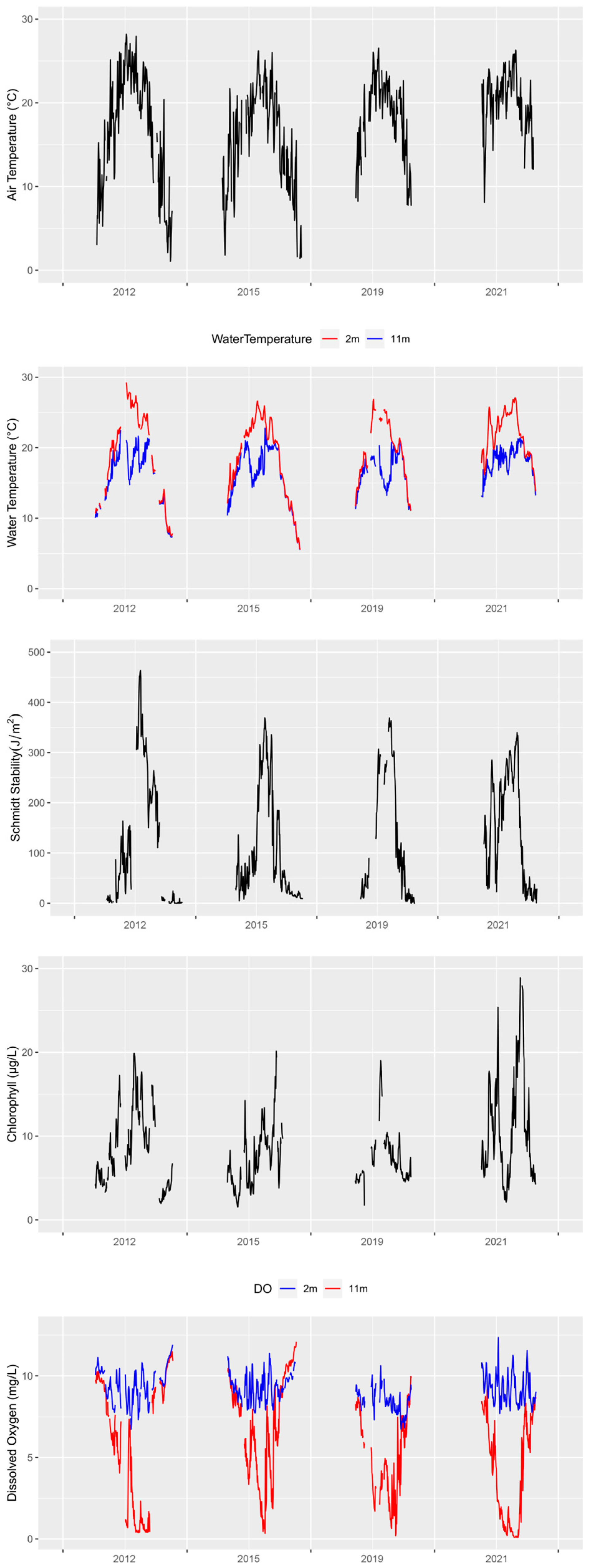
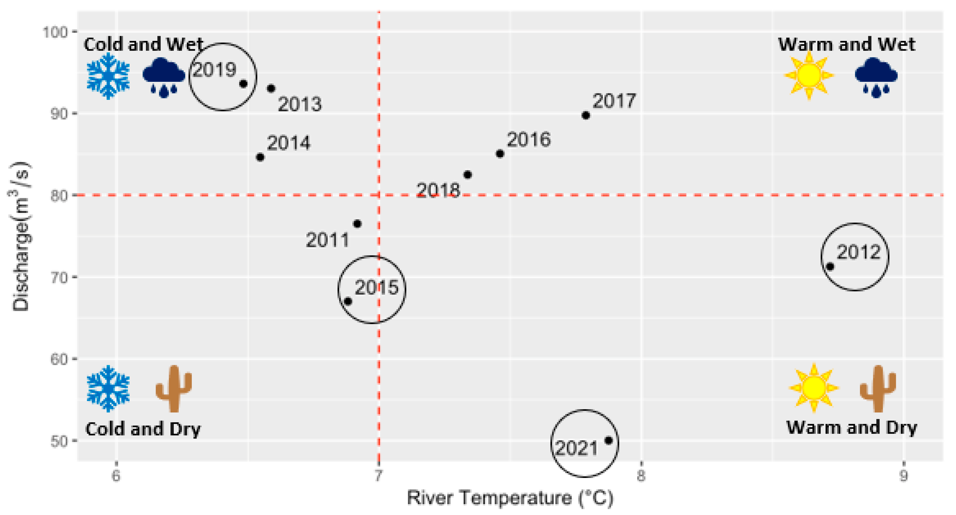
3.1. Environmental Drivers

Time-series graphs of air temperature and surface water temperature revealed a potential connection between these environmental variables and the severity of hypoxia. Less river discharge and higher springtime air and surface water temperatures were correlated with severe hypoxic years, and the opposite was true for mild hypoxic years (Table S1). Longer durations of high chlorophyll conditions signaled a potential excess amount of organic matter infiltrating the hypolimnion, leading to hypoxia, especially during years with stronger or longer durations of stratification (Figure 4 and Figure S2). Eutrophication, riverine discharge, and the temperature of the water column and overlying air coincided with the intensity of hypolimnetic hypoxia in the hypolimnion.

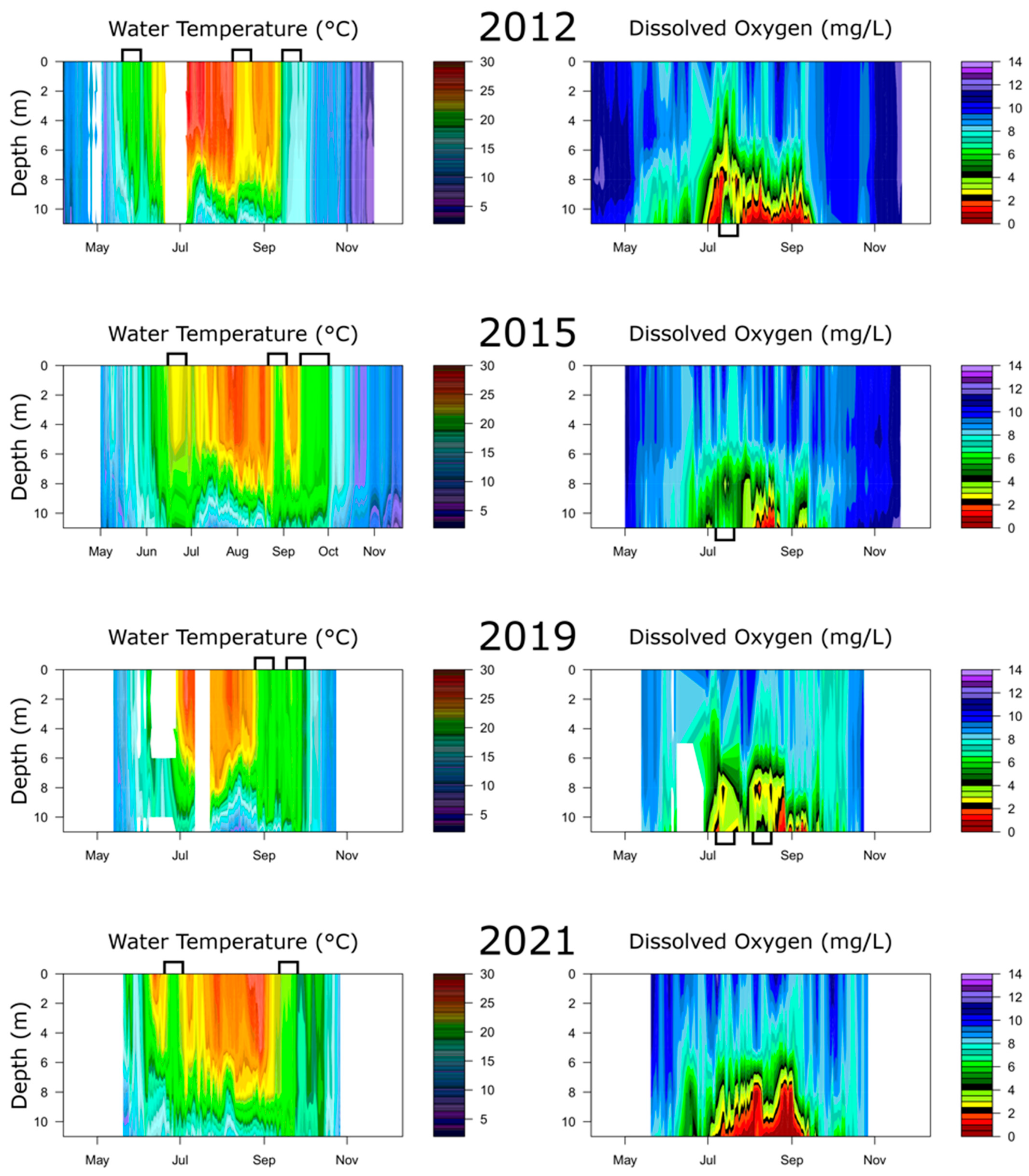
3.2. Comparison of Heat Maps

Heat maps illustrate the variation in stratification and hypoxia across the years. The severity of hypoxia differs greatly on a year-to-year basis, as does the thermal structure that serves as a prelude to hypolimnetic hypoxia in Muskegon Lake. The thermocline and oxycline tended to hover consistently around 6 m depth when hypoxia was most prevalent (Figure 5 and Figure S3). The duration of severe hypoxia was prolonged in the years 2011, 2012, 2016, 2018, and 2021 (Figure 5 and Figure S3). Severe hypoxia was also exacerbated in years with warmer surface temperatures in May and June compared to mild hypoxic years. Increased wind-mixing events and lower surface temperatures correlated with mild hypoxia compared to years with reduced wind-mixing, a more stratified water column, and warmer surface temperatures that correlated with severe hypoxia. A previous study in Muskegon Lake quantified a wind mixing event that deepened the epilimnion by approximately 1.5 m when westerly or southwesterly winds persisted at 7.7 m/s and for at least 10 h [45], so although wind mixing events can relieve some hypoxia from the upper hypolimnion, complete alleviation of hypoxia during summer stratification typically does not occur. Additionally, floating hypoxia, a phenomenon where low DO waters are moved up in the water column and separated from the sediment as cold, dense, oxygenated water from Lake Michigan wedges under the bottom of the hypolimnetic layer, occurs annually but most noticeably following cold water intrusions in 2011, 2013, 2015, 2016, 2018, and 2021 (Figure 5 and Figure S3) [35]. During these intrusion phenomena, the heat maps depict DO concentrations at 8 m depth to be lower than those at 11 m depth. Intrusions can be masked on the stratification heat maps as the cold Lake Michigan water can be of similar temperatures to the hypolimnetic water of Muskegon Lake.

3.3. Comparison of Stratification Strength and Duration

The Schmidt stability values varied greatly on a year-to-year basis. The onset of stratification according to the Schmidt stability values began as early as May (Table S2). The severely hypoxic years of 2011 and 2012 saw peaks of stratification strength above 400 J m−2, whereas another severely hypoxic year, 2021, had prolonged stratification beginning in June with comparatively fewer mixing events than other mild hypoxic years (Figure S4). Mildly hypoxic years tended to peak in stratification strength in mid-August or late July and had lower overall Schmidt stability values, peaking between 350 and 400 J m−2 (Figure S4). However, severely hypoxic years had Schmidt stability values peak in July. Almost every year, the fall lake turnover occurs in early to mid-October. An early onset of stratification and a higher intensity of stratification, as indicated by Schmidt stability indices, resulted in severe hypoxic years (Table 1 and Table S2). Meanwhile, a later onset of stratification and lower Schmidt stability values subsequently resulted in mild hypoxia (Table S2). It should be pointed out that 2015 and 2019 had the shortest duration of stratification, with 54 and 61 days, respectively. Additionally, 2016 and 2018 had the longest duration of stratification, with 122 and 114 days, respectively (Table 1). The earliest onset of stratification occurred in 2021 on May 20th, and the latest onset of stratification happened in 2015 on July 4th, suggesting that the time of the onset of stratification may play a larger role in hypoxia dynamics than the duration itself (Table S2). The missing data from 2018 was due to the sensor malfunctioning. However, the available data indicate that it was a year with a high potential for severe hypoxia. The 2020 field season was shortened due to the COVID-19 epidemic.

3.4. Hypoxia Severity Index

The hypoxia severity index showed that over the decade of MLO monitoring, the most hypoxic years occurred in 2012 and 2021, while 2011, 2013, 2016, 2017, and 2018 were moderately hypoxic years, and 2014, 2015, and 2019 were mildly hypoxic years (Table 1 and Table S3). From the hypoxic index, 2021 and 2012 were determined to be the most severely hypoxic years, with values of 97.06 and 91.27, respectively (Table 1). It should be mentioned that 2015 and 2019 were found to be the most mildly hypoxic years at 20.95 and 25.86, respectively (Table 1). The linear regression determined that hypoxia severity was neither increasing nor decreasing from 2011–2021 (p = 0.894). Similarly, a Pearson correlation was conducted and determined there is a very weak correlation between time and severity of hypoxia (0.049). Additionally, 2020 was removed from the hypoxia index due to the lack of data resulting from the COVID-19 pandemic.
Mild hypoxia at 8 m had the highest occurrences in 2012 and 2013, with 31 and 33 hypoxic days, respectively. Additionally, it had the lowest occurrences in 2015 and 2017, with 12 and 8 hypoxic days, respectively (Table 1 and Table S3). Severe hypoxia at 8 m had the highest incidence in 2011 and 2018, with 40 and 22 hypoxic days, respectively. Moreover, it had the lowest occurrence in 2014 and 2015, with 0 hypoxic days, respectively (Table 1). Near anoxia transpired at 8 m in 3 years only: 2011 (8 days), 2016 (2 days), and 2021 (1 day). At 11 m depth, mild hypoxia had the highest incidence in 2013 and 2019, with 52 and 45 hypoxic days, respectively. Furthermore, it had the lowest incidence in 2012 and 2018, with 6 and 8 days, respectively. Severe hypoxia occurred with the highest incidence during 2013 and 2016, with 40 and 42 hypoxic days, respectively. Additionally, severe hypoxia occurred with the lowest incidence in 2014 and 2015, with 13 and 15 hypoxic days, respectively (Table 1). Meanwhile, near anoxia was observed with the highest occurrence at 11 m depth in 2012 and 2021, with 19 and 28 near anoxic days, respectively (Table 1). Near anoxia was not detected in 2013 and 2014 at 11 m depth (Table 1). There was a portion of missing data during the field season every year except in 2017 and 2021.
Complete anoxia (0 mg/L) is difficult to detect with the daily averages of DO in the MLO dataset as DO fluctuates on a daily cycle. In the histogram of DO concentrations below 1 mg/L across the decade, 2021 was the only year that recorded complete anoxia, which lasted for 3 days (Figure S5). Additionally, 2012 and 2021 observed the longest duration of near anoxia as well as the most severe near anoxic conditions (Figure S5). The findings within the histogram coincide with the hypoxia index, where the most hypoxic years also experienced the most near-anoxic days.
The multiple linear regression determined that integrated precipitation over a majority of the watershed in the form of river discharge at the Croton Dam and river temperature prior to the onset of stratification and hypoxia drive the severity of hypoxia on an annual scale. The model was significant, with a p-value of 0.008 and an adjusted R2 of 0.899. River temperature had a p-value of 0.003 and a positive correlation, indicating that warmer river temperatures in the winter and spring precede a more hypoxic summer. River discharge had a negative correlation with the hypoxia severity index, with a significant p-value of 0.02. The standard residual error of the model was 0.16. The years were then grouped into four categories: cold and wet, cold and dry, hot and wet, and hot and dry. There was no significant trend (R2 = 0.1545) of river temperature versus discharge across the decade, although 7 of the 11 years had above-average discharge for the decade (Figure 6).
The PCA determined that July and August were closely related to surface temperature and Schmidt stability in Muskegon Lake. The hypoxia severity index was weakly correlated with all four environmental variables (Figure 7). The first two principal components were responsible for 73.25% of the cumulative data. September and October were not strongly correlated with any environmental variables.

4. Discussion

4.1. Variable Inter- and Intra-Annual Hypoxia

Previous work determined that hypoxia was an annually recurring feature of Muskegon Lake from 2011–2013, and the present study supports that finding with a decade of data [10]. However, there was no discernable trend in whether Muskegon Lake experienced increases or decreases in hypoxia over the decade, as hypoxia fluctuated considerably from year to year based on the environmental conditions during any particular year. The number of hypoxic days and the severity of hypoxia varied greatly throughout the decade as differing winter and spring precipitation likely led to differing nutrient and organic matter inputs to Muskegon Lake, which may ultimately drive hypoxia. Indeed, several earlier studies have revealed that Muskegon Lake is a net sink for both inorganic nutrients and organic matter received from the Muskegon River, which helps explain how riverine, nutrient-fueled excess phytoplankton production and organic matter-fueled respiration within the lake may contribute to variable bottom water hypoxia [6,7,28,37,50,51]. Therefore, eutrophication was a major issue during dry and severely hypoxic years as the residence time within Muskegon Lake lengthened. Observed changes in increased hypoxia severity were correlated with warmer air and surface water temperatures, as well as increased solar radiation possibly related to climate change [52]. In years with severe hypoxia, Muskegon Lake could fall victim to internal P loading (and presumably denitrification—not measured in the present study) and the release of greenhouse gasses, while reducing the capacity of the lake to act as a sink for nutrients and carbon [53,54]. Multiple stressors and their interactions can push ecosystems from their current stable states into alternative stable states [55,56,57]. A regime shift in the Muskegon Lake ecosystem is a possibility, as the surface waters could shift from a net sink to a net source of greenhouse gas emissions [51,53]. The high variability between years and relatively short time scales suggest that using this trend to extrapolate future conditions is not advisable. Rather, examining the environmental conditions prior to the onset of hypoxia and stratification can play a vital role in understanding the potential severity of hypoxia for any particular year. However, investigating the environmental conditions on a yearly basis can help to further understand the effects of climate change on hypoxic conditions.

4.2. Temperature-Precipitation Regime Regulates Hypoxia

As local and global climates continue to change, so do the anthropogenic influences exacerbating hypoxia [58,59,60,61,62]. The Great Lakes region is expected to continue warming while receiving overall increased precipitation, although seasonally variable, in the form of stronger storm events throughout the next century, especially in the spring and fall [17,63]. Muskegon Lake did not show an overall decadal trend in surface temperature at 2 m depth, but the yearly variance of river temperatures corresponded with the onset and severity of hypoxia. Other studies have also found that warm winter and spring temperatures resulted in an earlier onset of stratification, and warmer summer temperatures deepened the thermocline in temperate lakes [64,65,66]. Years with an early onset of stratification lead to a longer duration of oxygen depletion, while a deepened thermocline reduces the volume of water in the hypolimnion, resulting in less space in the water column to experience oxygen depletion. However, cooler air and surface water temperatures in the winter and spring can diminish the potential for hypoxia later in the year by delaying the onset of stratification, as demonstrated by the observations made in Muskegon Lake in 2014, 2015, and 2019. A study in Cape Cod Bay found that climate change-induced warming drastically expanded the hypoxic zone spatially through the water column during a year with extreme warming of air temperatures during the spring and summer [67]. In the United States, climatological shifts in weather patterns, such as the early onset of spring or a longer duration of spring conditions, can increase inland water temperatures, exacerbating hypoxia [68]. The warmer winter and spring river temperatures in the Muskegon River suggest that this may be partially responsible for the severe hypoxia experienced during the years 2012 and 2021.
Similarly, increased precipitation in the spring can lead to decreased zones of hypoxia by weakening or delaying stratification and shortening the residence time in the estuary despite carrying more nutrients from upstream [69,70]. Years with extensive precipitation during the spring and early summer led to increased nutrient runoff and eutrophication of Muskegon Lake but reduced the residence time, potentially reducing hypoxia [70]. A study comparing global estuaries determined that coastal estuaries with longer residence times, such as the Gulf of St. Lawrence and the Chesapeake Bay, experience more severe hypoxia than systems with shorter residence times, such as the Pearl River [71]. Lakes that retain nutrients also experience increased eutrophication as nutrients remain in the system for an extended period [72,73]. Despite increased eutrophication during years with increased precipitation, the shortened residence time within Muskegon Lake may have reduced primary productivity at the surface, even though Muskegon Lake historically retains approximately one-third of the phosphorus that enters the lake before exiting into Lake Michigan [28]. Recent work [74] has shown a trend of increasing the number of days experiencing liquid precipitation over the last 60 years across the U.S., thus leading to lower severity of hypoxia in these heavy precipitation years. Increasing drought and heat wave frequency across the U.S. could promote more severe hypoxic conditions, similar to those observed in 2012 and 2021 in Muskegon Lake [21,74]. Monitoring seasonal precipitation and river loading is important for understanding the severity of hypoxia on a yearly basis.

4.3. Role of Surface Production and Hypolimnetic Respiration

Warm spring and summer water temperatures further create conditions that promote bloom-forming cyanobacteria [61,75]. An increase in surface productivity has been linked to increased hypoxia and acidification during summer surface blooms in two eutrophic estuaries on western Long Island Sound, NY, reshaping the food webs due to the combined effect of hypoxia and acidification [22]. Sinking surface biomass into the hypolimnion drives oxygen depletion through microbial respiration associated with the decomposition process. The severely hypoxic years experienced in Muskegon Lake were associated with elevated chlorophyll-a concentrations, a pigment that is inclusive of all algae, though other work conducted on Muskegon Lake has shown that years with greater chlorophyll-a levels correlate with greater cyanobacterial biomass specifically [76]. Air temperature also appears to have an influence on both surface and bottom water temperatures. Greater surface water temperatures are one of the environmental conditions promoted by increased air temperatures that encourage the growth of bloom-forming algae—particularly cyanobacteria—while simultaneously acting to increase the thermal gradient between the epilimnion and hypolimnion, diminishing the vertical transport of dissolved oxygen from the epilimnion to the hypolimnion [62,77]. Overall, the findings from the above two subsections indicate that temperature and precipitation regulate hypoxia dynamics in Muskegon Lake, which aligns with their recognized roles as important variables in the Earth system [17,74,78].

4.4. Potential Release and Role of Legacy Phosphorus in Sediment

Internal phosphorus loading (IPL) is the release of legacy-bound phosphorus during anoxic conditions in the hypolimnion when phosphorus desorbs from the sediment [51]. Following such phosphorus releases from the sediment, wind mixing events can mix the water column and bring it to the surface, where phytoplankton may bloom in a previously phosphorus-limited environment. A previous study that quantified phosphorus in the water column determined that IPL appears to have occurred in Muskegon Lake in 2021 following anoxic conditions in the hypolimnion and a wind mixing event. This led to a measurable increase in the development of cyanobacterial blooms approximately one month following the initial detection of IPL-derived soluble reactive phosphorus in the surface water [79]. In years where hypoxia is extremely severe and even anoxic, such as 2021, IPL loading may further exacerbate the hypoxic conditions within an ecosystem, leading to degradation of surface and bottom waters—the latter through a positive feedback loop wherein IPL leads to sinking surface blooms that further worsen hypolimnetic hypoxia, and so on. The exact source of phosphorus in the bottom waters of Muskegon Lake is unknown at this time, as research that indicates that IPL may be occurring [7,79] conflicts with other research that suggests IPL does not occur in Muskegon Lake [51]. Further research is needed to quantify the variable IPL in inland waters and its role as a positive feedback loop under future anthropogenic pressures and climate change scenarios.

4.5. Complexities of Hypoxia Dynamics and Management Implications

Estuary ecosystems are highly complex and dynamic, and as such, there are several environmental variables that work to alter the hypoxic zone’s duration and depth. Other factors, such as wind mixing events, also impact water column stratification and nutrient input into the hypolimnion, both of which can lead to the disruption or formation of hypoxia [80,81]. An earlier study in 2015 found that even severe and sustained wind events were unable to completely mix the hypolimnion during the summer stratified period in Muskegon Lake [45]. Furthermore, strong wind events coming from the north and northwest have been found to cause the upwelling of cold, oxygenated water from Lake Michigan into Muskegon Lake and Green Bay, which acts to temporarily alter hypoxic conditions [35,45,81]. Intrusions of such cold and oxygenated upwelled water from nearshore displace the hypoxic water from contact with the lake bottom and force it shallower in the water column, leading to floating hypoxia. Floating hypoxia can also restrict the habitat of fish species and produce increased predation and overfishing [82,83,84]. Although the consequences of wind mixing events and floating hypoxia are short on the temporal scale, the repetition and severity of the events generate a strained ecosystem characterized by a dynamic hypolimnetic hypoxia regime.
Historical management of hypoxia has been conducted through nutrient reductions in respective watersheds [85]. While these nutrient abatements initially proved successful, re-eutrophication despite nutrient reductions has brought forth continued hypoxic conditions and subsequent consequences at the surface and in the hypolimnion [86,87]. The results of this study suggest that watershed management on an annual scale should consider forecasted precipitation and air temperature to assess the extent and severity of hypoxia. For instance, nutrient abatements may need to be increased in years where particularly warm spring and summer conditions as well as higher precipitation are expected. Understanding the long-term trends of hypoxia is also valuable for managers in the face of climate change. However, these long-term trends may not provide as much information as the environmental conditions within a given year.

5. Conclusions

Bottom-water hypoxia is rapidly expanding as the Earth continues to warm and anthropogenic land use changes increasingly contribute to cultural eutrophication. Muskegon Lake, a mesotrophic Great Lakes estuary, experiences hypoxia on a yearly basis. Our study, utilizing time-series data from a high-frequency lake observatory, provides detailed insight into the dynamics of hypoxia in a Great Lakes estuary throughout a decade as well as the environmental conditions that drive hypoxia during any particular year. The severity of hypoxia did not have a discernible inter-annual trend over the decade of study. Hypoxia was most severe in years with greater strength, an earlier onset, or a longer duration of stratification. In general, lower discharge rates and warmer water and air temperatures in the winter and spring, coupled with fewer wind mixing events, led to more severe and longer durations of hypoxia in the ensuing summer-fall period. On the other hand, years with greater discharge, cooler water and air temperatures, and greater wind mixing events during the spring and early summer experienced milder hypoxic conditions both temporally and spatially. Thus, knowledge of the environmental conditions prior to the onset of hypoxia can be useful in predicting the potential severity of hypoxia for any particular year.
Our findings suggest that variable temperature and precipitation are major drivers of hypoxia and that changes in these key variables can lead to further deoxygenation of the lake’s interior. As the global water cycle amplifies under a warming climate with an increased incidence of extreme weather, consequences to consider for the future of hypoxia globally include effects on the food web and the carbon cycle, as well as impacts on recreational and social reliance upon these freshwater resources [14,78,88,89]. Thus, closer monitoring of aquatic ecosystems is critical in the face of ongoing anthropogenic disturbances and climate change. Muskegon Lake, a model Great Lakes estuary with detailed chronicles of hypoxia over multiple years, can serve as a sentinel for deoxygenation in freshwater lakes, estuaries, and coastal waters everywhere.

Supplementary Materials

The following supporting information can be downloaded at: https://www.mdpi.com/article/10.3390/hydrobiology2020027/s1, Figure S1: Muskegon Lake Observatory gathering time-series meteorological and water quality data in Mus-kegon Lake, MI, USA; Figure S2: Time-series graphs of (A) air temperature, (B) surface water temperature, (C) Schmidt Stability, (D) surface chlorophyll-a at 2 m, and (E) DO at 2 m and 11 m from 2011–2021; Figure S3: Time-series heat maps of 2011–2021 thermal stratification and dissolved oxygen from the Muskegon Lake Observatory (MLO) buoy; Figure S4: Schmidt stability time-series graphs from 2011–2021; Figure S5: Histogram of DO intervals below the near anoxia threshold of 1 mg/L from 2011–2021; Table S1: Table of Muskegon River discharge and temperature values averaged from January–July 2011–2021, timetable prior to the onset of hypoxic; Table S2: The onset and disruption of stratification; Table S3: Chronologically ordered table illustrating the number of days where hypoxia was detected at a mild or severe level of hypoxia or near anoxia.

Author Contributions

Conceptualization, N.M.D., B.A.B. and A.D.W.; methodology, N.M.D., I.P.S., B.A.B. and A.D.W.; validation, N.M.D., B.A.B., A.D.W. and I.P.S.; formal analysis, N.M.D., A.D.W. and I.P.S.; investigation, N.M.D., I.P.S. and B.A.B.; resources, B.A.B. and N.M.D.; data curation, A.D.W., B.A.B., N.M.D. and I.P.S.; writing—original draft preparation, N.M.D., B.A.B., A.D.W. and I.P.S.; writing—review and editing, I.P.S., A.D.W. and B.A.B.; visualization, N.M.D., A.D.W., I.P.S. and B.A.B.; supervision, B.A.B.; project administration, N.M.D. and B.A.B.; funding acquisition, B.A.B. and N.M.D. All authors have read and agreed to the published version of the manuscript.

Funding

This research was funded by EPA-Great Lakes Restoration Initiative (R5-GL2010-1), NOAA-Cooperative Institute for Great Lakes Research (NA12OAR4320071), Community Foundation for Muskegon County (20172151), Consumers Energy (250700-40625-200), and NASA (Michigan Space Grant Consortium 80NSSC20M01244) grants. Dugener was supported by a Michigan Space Grant Consortium Fellowship and the Grand Valley State University Presidential Research Grant.

Institutional Review Board Statement

Not applicable.

Informed Consent Statement

Not applicable.

Data Availability Statement

The data presented in this study are openly available in the Environmental Data Initiative at https://doi.org/10.6073/pasta/d1ef6101a1870a0b0bd54d3914dc13dc, accessed on 30 October 2022, reference number edi.1044.1.

Acknowledgments

We are thankful to Scott Kendall for having played a major role in establishing the Muskegon Lake Observatory in 2011. We would like to acknowledge Jasmine Mancuso for her assistance with statistical analyses and Brain Scull for assistance with nutrient analyses.

Conflicts of Interest

The authors declare no conflict of interest.

References

  1. Breitburg, D.; Levin, L.A.; Oschlies, A.; Grégoire, M.; Chavez, F.P.; Conley, D.J.; Garçon, V.; Gilbert, D.; Gutiérrez, D.; Isensee, K.; et al. Declining oxygen in the global ocean and coastal waters. Science 2018, 359, 46. [Google Scholar] [CrossRef] [PubMed] [Green Version]
  2. Diaz, R.J.; Rosenberg, R. Spreading dead zones and consequences for marine ecosystems. Science 2008, 231, 926–929. [Google Scholar] [CrossRef] [PubMed]
  3. Ding, S.; Chen, M.; Gong, M.; Fan, X.; Qin, B.; Xu, H.; Gao, S.; Jin, Z.; Tsang, D.C.W.; Zhang, C. Internal phosphorus loading from sediments causes seasonal nitrogen limitation for harmful algal blooms. Sci. Total Environ. 2018, 625, 872–884. [Google Scholar] [CrossRef] [PubMed]
  4. Jane, S.F.; Hansen, G.J.A.; Kraemer, B.M.; Leavitt, P.R.; Mincer, J.L.; North, R.L.; Pilla, R.M.; Stetler, J.T.; Williamson, C.E.; Woolway, R.I.; et al. Widespread deoxygenation of temperate lakes. Nature 2021, 594, 66–81. [Google Scholar] [CrossRef]
  5. Rabalais, N.N.; Díaz, R.J.; Levin, L.A.; Turner, R.E.; Gilbert, D.; Zhang, J. Dynamics and distribution of natural and human-caused hypoxia. Biogeosciences 2010, 7, 585–619. [Google Scholar] [CrossRef] [Green Version]
  6. Scavia, D.; Allan, J.D.; Arend, K.K.; Bartell, S.; Beletsky, D.; Bosch, N.S.; Brandt, S.B.; Briland, R.D.; Daloğlu, I.; DePinto, J.V.; et al. Assessing and addressing the re-eutrophication of Lake Erie: Central basin hypoxia. J. Great Lakes Res. 2014, 40, 226–246. [Google Scholar] [CrossRef]
  7. Weinke, A.D.; Biddanda, B.A. From bacteria to fish: Ecological consequences of seasonal hypoxia in a Great Lakes estuary. Ecosystems 2018, 21, 426–442. [Google Scholar] [CrossRef] [Green Version]
  8. Magaud, H.; Migeon, B.; Morfin, P.; Garric, J.; Vindimian, E. Modelling fish mortality due to urban storm run-off: Interacting effects of hypoxia and unionized ammonia. Water Res. 1997, 31, 211–218. [Google Scholar] [CrossRef]
  9. Tellier, J.M.; Kalejs, N.I.; Leonhardt, B.S.; Cannon, D.; Höök, T.O.; Collingsworth, P. Widespread prevalence of hypoxia and the classification of hypoxic conditions in the Laurentian Great Lakes. J. Great Lakes Res. 2022, 48, 13–23. [Google Scholar] [CrossRef]
  10. Biddanda, B.A.; Weinke, A.D.W.; Kendall, S.T.; Gereaux, L.C.; Holcomb, T.M.; Snider, M.J.; Dila, D.K.; Long, S.A.; VandenBurg, C.; Knapp, K.; et al. Chronicles of hypoxia: Time-series buoy observations reveal annually recurring seasonal basin-wide hypoxia in Muskegon Lake—A Great Lakes estuary. J. Great Lakes Res. 2018, 44, 219–229. [Google Scholar] [CrossRef]
  11. Xu, W.; Collingsworth, P.D.; Kraus, R.; Minsker, B. Spatio-Temporal Analysis of Hypoxia in the Central Basin of Lake Erie of North America. Water Resour. Res. 2021, 57, e2020WR027676. [Google Scholar] [CrossRef]
  12. Klump, J.V.; Brunner, S.L.; Grunert, B.K.; Kaster, J.L.; Weckerly, K.; Houghton, E.M.; Kennedy, J.A.; Valenta, T.J. Evidence of persistent, recurring summertime hypoxia in Green Bay, Lake Michigan. J. Great Lakes Res. 2018, 44, 841–850. [Google Scholar] [CrossRef]
  13. Larson, J.H.; Trebitz, A.S.; Steinman, A.D.; Wiley, M.J.; Carlson Mazur, M.; Pebbles, V.; Braun, H.A.; Seelbach, P.W. Great Lakes rivermouth ecosystems: Scientific synthesis and management implications. J. Great Lakes Res. 2013, 39, 513–524. [Google Scholar] [CrossRef]
  14. Weinke, T.; Stone, I.; Greene, J.; Woznicki, S.; Cook, J.; Dugener, N.; Biddanda, B. Great Lakes Estuaries: Hot spots of productivity, problems, and potential. IAGLR Lakes Lett. 2022, 9–10. Available online: https://iaglr.org/ll/2022-3-Summer_LL14.pdf (accessed on 30 October 2022).
  15. Steinman, A.D.; Ogdahl, M.; Rediske, R.; Ruetz, C.R.; Biddanda, B.A.; Nemeth, L. Current status and trends in Muskegon Lake, Michigan. J. Great Lakes Res. 2008, 34, 169–188. [Google Scholar] [CrossRef]
  16. Rahmstorf, S.; Coumou, D. Increase of extreme events in a warming world. Proc. Natl. Acad. Sci. USA 2011, 108, 17905–17909. [Google Scholar] [CrossRef] [Green Version]
  17. Byun, K.; Hamlet, A.F. Projected changes in future climate over the Midwest and Great Lakes region using downscaled CMIP5 ensembles. Int. J. Climatol. 2018, 38, e531–e553. [Google Scholar] [CrossRef]
  18. Michalak, A.M. Study role of climate change in extreme threats to water quality. Nature 2016, 535, 349–350. [Google Scholar] [CrossRef] [Green Version]
  19. Whitney, M.M. Observed and forecasted global warming pressure on coastal hypoxia. Biogeosciences 2021, 19, 4479–4497. [Google Scholar]
  20. O’Reilly, C.M.; Sharma, S.; Gray, D.K.; Hampton, S.E.; Read, J.S.; Rowley, R.J.; Schneider, P.; Lenters, J.D.; McIntyre, P.B.; Kraemer, B.M.; et al. Rapid and highly variable warming of lake surface waters around the globe. AGUPublications 2015, 42, 10773–10781. [Google Scholar] [CrossRef] [Green Version]
  21. Tassone, S.J.; Besterman, A.F.; Buelo, C.D.; Ha, D.T.; Walter, J.A.; Pace, M.L. Increasing heatwave frequency in streams and rivers of the United States. Limnol. Oceanogr. 2023, 8, 295–304. [Google Scholar] [CrossRef]
  22. Wallace, R.B.; Gobler, C.J. The role of algal blooms and community respiration in controlling the temporal and spatial dynamics of hypoxia and acidification in eutrophic estuaries. Marine Pollut. Bull. 2021, 172, 112908. [Google Scholar] [CrossRef] [PubMed]
  23. Austin, J.A.; Colman, S.M. Lake Superior summer water temperatures are increasing more rapidly than regional air temperatures: A positive ice-albedo feedback. Geophys. Res. Lett. 2007, 34, L06604. [Google Scholar] [CrossRef] [Green Version]
  24. Winslow, L.A.; Read, J.S.; Hansen, G.J.A.; Rose, K.C.; Robertson, D.M. Seasonality of change: Summer warming rates do not fully represent effects of climate change on lake temperatures. Limno. Oceanogr. 2017, 62, 2168–2178. [Google Scholar] [CrossRef]
  25. Smith, V.H. Eutrophication of freshwater and coastal marine ecosystems, a global problem. Environ. Sci. Pollut. Res. 2003, 10, 126–139. [Google Scholar] [CrossRef] [PubMed]
  26. Paerl, H.W.; Valdes, L.M.; Peierls, B.L.; Adolf, J.E.; Harding, L.W., Jr. Anthropogenic and climatic influences on the eutrophication of large estuarine ecosystems. Limnol. Oceanogr. 2006, 51, 448–462. [Google Scholar] [CrossRef] [Green Version]
  27. Paerl, H.W.; Gardner, W.S.; Havens, K.E.; Joyner, A.R.; McCarthy, M.J.; Newell, S.E.; Qin, B.; Scott, J.T. Mitigating cyanobacterial harmful algal blooms in aquatic ecosystems impacted by climate change and anthropogenic nutrients. Harmful Algae 2016, 54, 213–222. [Google Scholar] [CrossRef] [Green Version]
  28. Marko, K.M.; Rutherford, E.S.; Eadie, B.J.; Johengen, T.H.; Lansing, M.B. Delivery and seston from the Muskegon River Watershed to nearshore Lake Michigan. J. Great Lakes Res. 2013, 39, 672–681. [Google Scholar] [CrossRef]
  29. Dodds, W.K.; Bouska, W.W.; Eitzmann, J.L.; Pilger, T.J.; Pitts, K.L.; Riley, A.J.; Schloesser, J.T.; Thornbrugh, D.L. Eutrophication of U.S. freshwaters: Analysis of potential economic damages. Environ. Sci. Technol. 2008, 43, 12–19. [Google Scholar] [CrossRef] [Green Version]
  30. Salk, K.R.; Venkitswaran, J.J.; Couture, R.; Higgins, S.N.; Paterson, M.J.; Schiff, S.L. Warming combined with experimental eutrophication intensifies lake phytoplankton blooms. Limnol. Oceanogr. 2021, 67, 147–158. [Google Scholar] [CrossRef]
  31. Burkholder, J.M.; Kinder, C.A.; Dickey, D.A.; Reed, R.E.; Arellano, C.; James, J.L.; Mackenzie, L.M.; Allen, E.H.; Lindor, N.L.; Mathis, J.G.; et al. Classic indicators and diel dissolved oxygen versus trend analysis in assessing eutrophication of potable-water reservoirs. Ecol. Appl. 2022, 32, e2541. [Google Scholar] [CrossRef] [PubMed]
  32. Kim, M.S.; Kim, K.H.; Hwang, S.J.; Lee, T.K. Role of Algal Community Stability in Harmful Algal Blooms in River-Connected Lakes. Microbial Ecol. 2021, 82, 309–318. [Google Scholar] [CrossRef] [PubMed]
  33. Williamson, C.E.; Saros, J.E.; Vincent, W.F.; Smol, J.P. Lakes and reservoirs as sentinels, integrators, and regulators of climate change. Limnol. Oceanogr. 2009, 54, 2273–2282. [Google Scholar] [CrossRef]
  34. Freedman, P.; Canale, R.; Auer, M. The Impact of Wastewater Diversion Spray Irrigation on Water Quality in Muskegon County Lakes; U.S. Environmental Protection Agency: Washington, DC, USA, 1979; 905/9–79–006-A. [Google Scholar]
  35. Liu, Q.; Anderson, E.J.; Zhang, Y.; Weinke, A.D.; Knapp, K.L.; Biddanda, B.A. Modeling reveals the role of coastal upwelling and hydrologic inputs on biologically distinct water exchanges in a Great Lakes estuary. Estuar. Coast. Shelf Sci. 2018, 209, 41–55. [Google Scholar] [CrossRef]
  36. Biddanda, B.; Kendall, S.; Weinke, A.; Stone, I.; Dugener, N.; Ruberg, S.; Leidig, J.; Smith, E.; Berg, M.; Wolffe, G. Muskegon Lake Observatory Buoy Data: Muskegon Lake, Michigan: 2011–2019 ver 1. Environmental Data Initiative. Available online: https://doi.org/10.6073/pasta/d1ef6101a1870a0b0bd54d3914dc13dc (accessed on 30 October 2022).
  37. Mancuso, J.L.; Weinke, A.D.; Stone, I.P.; Hamsher, S.E.; Villar-Argaiz, M.; Biddanda, B.A. Cold and wet: Diatoms dominate the phytoplankton community during a year of anomalous weather in a Great Lakes estuary. J. Great Lakes Res. 2021, 47, 1305–1315. [Google Scholar] [CrossRef]
  38. Winslow, L.; Read, J.; Woolway, R.; Brentrup, J.; Leach, T.; Zwart, J.; Albers, S.; Collinge, D. rLakeAnalyzer: Lake Physics Tools, R package version 1 (11). 2015. Available online: https://rdrr.io/cran/rLakeAnalyzer/ (accessed on 30 October 2022).
  39. Read, J.S.; Hamilton, D.P.; Jones, I.D.; Muraoka, K.; Winslow, L.A.; Kroiss, R.; Wu, C.H.; Gaiser, E. Derivation of lake mixing and stratification indices from high-resolution lake buoy data. Environ. Model. Softw. 2011, 26, 1325–1336. [Google Scholar] [CrossRef]
  40. Nürnberg, G.K. Quantifying anoxia in lakes. Limnol. Oceanogr. 1995, 40, 1100–1111. [Google Scholar] [CrossRef]
  41. Matthews, D.A.; Effler, S.W. Long-term changes in the areal hypolimnetic oxygen deficit (AHOD) of Onondaga Lake: Evidence of sediment feedback. Limnol. Oceanogr. 2006, 51, 702–714. [Google Scholar] [CrossRef]
  42. Foley, B.; Jones, I.D.; Maberly, S.C.; Rippey, B. Long-term changes in oxygen depletion in a small temperate lake: Effects of climate change and eutrophication. Freshw. Biol. 2012, 57, 278–289. [Google Scholar] [CrossRef]
  43. Nürnberg, G.K. Quantification of Oxygen Depletion in Lakes and Reservoirs with the Hypoxic Factor. Lake Reserv. Manag. 2002, 18, 299–306. [Google Scholar] [CrossRef]
  44. USGS Muskegon River Near Croton, MI. Available online: https://waterdata.usgs.gov/monitoring-location/04121970/#parameterCode=00060&period=P365D. (accessed on 7 December 2022).
  45. Weinke, A.D.; Biddanda, B.A. Influence of episodic wind events on thermal stratification and bottom water hypoxia in a Great Lakes estuary. J. Great Lakes Res. 2019, 45, 1103–1112. [Google Scholar] [CrossRef]
  46. R Core Team. R: A Language and Environment for Statistical Computing; R Foundation for Statistical Computing: Vienna, Austria, 2018. [Google Scholar]
  47. Wickham, H. ggplot2: Elegant Graphics for Data Analysis; Springer: New York, NY, USA, 2016. [Google Scholar]
  48. Wickham, H.; François, R.; Henry, L.; Müller, K. dplyr: A Grammar of Data Manipulation, R package version 0.7.5. 2018. Available online: https://cran.r-project.org/web/packages/dplyr/index.html (accessed on 30 October 2022).
  49. Verzani, J. UsingR: Data Sets, Etc. For the Test “Using R for Introductory Statistics”, R Package Version 2.0-6, 2nd ed. 2018. Available online: https://cran.r-project.org/web/packages/UsingR/UsingR.pdf (accessed on 30 October 2022).
  50. Defore, A.L.; Weinke, A.D.; Lindback, M.M.; Biddanda, B.A. Year-round measures of planktonic metabolism reveal net autotrophy in surface waters of a Great Lakes estuary. Aquat. Microb. Ecol. 2016, 77, 139–153. [Google Scholar] [CrossRef] [Green Version]
  51. Steinman, A.D.; Spears, B.M. Internal Phosphorus Loading in Lakes: Causes, Case Studies, and Management; J. Ross Publishing: Plantation, FL, USA, 2020. [Google Scholar]
  52. Schmid, M.; Read, J. Heat Budget of Lakes. Reference Module In Earth Systems and Environmental Sciences; Encyclopedia of Inland Waters: Amsterdam, The Netherlands, 2021; Volume 7. [Google Scholar]
  53. Salk, K.R.; Ostrom, P.H.; Biddanda, B.A.; Weinke, A.D.; Kendall, S.T.; Ostrom, N.E. Ecosystem metabolism and greenhouse gas production in a mesotrophic northern temperate lake experiencing seasonal hypoxia. Biogeochem. 2016, 131, 303–319. [Google Scholar] [CrossRef]
  54. Carey, C.C.; Hanson, P.C.; Thomas, R.Q.; Gerling, A.B.; Hounshell, A.G.; Lewis, A.S.L.; Lofton, M.E.; McClure, R.P.; Wander, H.L.; Woelmer, W.M.; et al. Anoxia decreases the magnitude of the carbon, nitrogen, and phosphorus sink in freshwaters. Global Chang. Biol. 2022, 28, 4861–4881. [Google Scholar] [CrossRef] [PubMed]
  55. Villar-Argaiz, M.; Medina-Sánchez, J.M.; Biddanda, B.A.; Carrillo, P. Predominant Non-additive Effects of Multiple Stressors on Autotroph C:N:P Ratios Propagate in Freshwater and Marine Food Webs. Front. Microbiol. 2018, 9, 69. [Google Scholar] [CrossRef] [PubMed] [Green Version]
  56. Scheffer, M.; Carpenter, S.R.; Lenton, T.M.; Bascompte, J.; Brock, W.; Dakos, V.; Van De Koppel, J.; Van De Leemput, I.A.; Levin, S.A.; Van Nes, E.H.; et al. Anticipating Critical Transitions. Science 2012, 338, 344–348. [Google Scholar] [CrossRef] [Green Version]
  57. Scheffer, M.; Jeppesen, E. Alternative Stable States. Ecol. Studies 1998, 131, 397–406. [Google Scholar]
  58. Schneider, P.; Hook, S.J. Space observations of inland waterbodies show rapid surface warming since 1985. Geophys. Res. 2010, 37, L22405. [Google Scholar]
  59. Dokulil, M.T. Impact of climate warming on European inland waters. Inland Waters 2014, 4, 27–40. [Google Scholar] [CrossRef]
  60. Jenny, J.-P.; Francus, P.; Normandeau, A.; Lapointe, F.; Perga, M.-E.; Ojala, A.; Schimmelmann, A.; Zolitschka, B. Global spread of hypoxia in freshwater ecosystems during the last three centuries is caused by rising local human pressure. Global Chang. Biol. 2016, 22, 1481–1489. [Google Scholar] [CrossRef]
  61. Paerl, H.W.; Huisman, J. Blooms like it hot. Science 2008, 320, 57–58. [Google Scholar] [CrossRef] [PubMed] [Green Version]
  62. Meire, L.; Soetaert, K.E.R.; Meysman, F.J.R. Impact of global change on coastal oxygen dynamics and risk of hypoxia. Biogeosciences 2013, 10, 2633–2653. [Google Scholar] [CrossRef] [Green Version]
  63. Hayhoe, K.; VanDorn, J.; Croley, T.; Schlegal, N.; Wuebbles, D. Regional climate change projections for Chicago and the US Great Lakes. J. Great Lakes Res. 2010, 36, 7–21. [Google Scholar] [CrossRef]
  64. Hondzo, M.; Stefan, H.G. Three case studies of lake temperature and stratification response to warmer climate. Water Resour. Res. 1991, 27, 1837–1848. [Google Scholar] [CrossRef]
  65. Del Giudice, D.; Zhou, Y.; Sinha, E.; Michalak, A.M. Long-term phosphorous loading and springtime temperatures explain interannual variability of hypoxia in a large temperate lake. Environ. Sci. Technol. 2018, 52, 2046–2054. [Google Scholar] [CrossRef] [PubMed]
  66. Sahoo, G.B.; Schladow, S.G.; Reuter, J.E.; Coats, R. Effects of climate change on thermal properties of lakes, reservoirs, and possible implications. Stoch. Environ. Res. Risk Assess. 2011, 25, 445–456. [Google Scholar] [CrossRef] [Green Version]
  67. Scully, M.E.; Geyer, W.R.; Borkman, D.; Pugh, T.L.; Costa, A.; Nichols, O.C. Unprecedented Summer Hypoxia in Southern Cape Cod Bay: An Ecological Response to Regional Climate Change? Biogeosciences 2022, 19, 3523–3536. [Google Scholar] [CrossRef]
  68. Pal, I.; Anderson, B.T.; Salvucci, G.D.; Gianatti, D.J. Shifting seasonality and increasing frequency of precipitation in wet and dry seasons across the U.S. Geophys. Res. Lett. 2013, 40, 4030–4035. [Google Scholar] [CrossRef]
  69. Crockford, L.; Jordan, P.; Melland, A.R.; Taylor, D. Storm-triggered, increased-supply of sediment-derived phosphorus to the epilimnion in a small freshwater lake. Inland Waters 2015, 5, 15–26. [Google Scholar] [CrossRef] [Green Version]
  70. Bouffard, D.; Ackerman, J.D.; Boegman, L. Factors affecting the development and dynamics of hypoxia in a large shallow stratified lake: Hourly to seasonal patterns. Water Resour. Res. 2013, 49, 2380–2394. [Google Scholar] [CrossRef] [Green Version]
  71. Fennel, K.; Testa, J.M. Biogeochemical Controls on Coastal Hypoxia. Annu. Rev. Mar. Sci. 2019, 11, 105–130. [Google Scholar] [CrossRef] [PubMed]
  72. Watson, S.B.; Miller, C.; Arhonditsis, G.; Boyer, G.L.; Carmichael, W.; Charlton, M.N.; Confesor, R.; Depew, D.C.; Höök, T.O.; Ludsin, S.A.; et al. The re-eutrophication of Lake Erie: Harmful algal blooms and hypoxia. Harmful Algae 2016, 56, 44–66. [Google Scholar] [CrossRef]
  73. Edwards, W.J.; Conroy, J.D.; Culver, D.A. Hypolimnetic Oxygen Depletion Dynamics in the Central Basin of Lake Erie. J. Great Lakes Res. 2005, 31, 262–271. [Google Scholar] [CrossRef]
  74. Harp, R.D.; Horton, D.E. Observed changes in daily precipitation intensity in the United States. Geophys. Res. Lett. 2022, 49, e2022GL099955. [Google Scholar] [CrossRef]
  75. Deng, J.; Qin, B.; Paerl, H.; Zhang, Y.; Ma, J.; Chen, Y. Earlier and warmer springs increase cyanobacterial (Microcystis spp.) blooms in subtropical Lake Taihu, China. Freshw. Biol. 2014, 59, 1076–1085. [Google Scholar] [CrossRef]
  76. Gillett, N.M.D.; Steinman, A.D. An analysis of long-term phytoplankton dynamics in Muskegon Lake—A Great Lakes Area of Concern. J. Great Lakes Res. 2011, 37, 335–342. [Google Scholar] [CrossRef]
  77. Bocaniov, S.A.; Lamb, K.G.; Liu, W.; Rao, Y.R.; Smith, R.E.H. High sensitivity of lake hypoxia to air temperatures, winds, and nutrient loading: Insights from a 3-D lake model. Water Resour. Res. 2020, 56, e2019WR027040. [Google Scholar] [CrossRef]
  78. Schlesinger, W.H.; Bernhardt, E.S. Biogeochemistry: An Analysis of Global Change, 3rd ed.; Academic Press: Cambridge, MA, USA, 2013. [Google Scholar]
  79. Dugener, N.M.; Stone, I.P.; Weinke, A.D.; Biddanda, B.A. Out of oxygen: Stratification and loading drove hypoxia during a warm, wet, and productive year in a Great Lakes estuary. J. Great Lakes Res. 2023. submitted. [Google Scholar]
  80. Jabbari, A.; Ackerman, J.D.; Boegman, L.; Zhao, Y. Episodic hypoxia in the western basin of Lake Erie. Limnol. Oceanogr. 2019, 64, 2220–2236. [Google Scholar] [CrossRef]
  81. Hamidi, S.A.; Bravo, H.R.; Klump, J.V.; Waples, J.T. The role of circulation and heat fluxes in the formation of stratification leading to hypoxia in Green Bay, Lake Michigan. J. Great Lakes Res. 2015, 41, 1024–1036. [Google Scholar] [CrossRef]
  82. Grunert, B.K.; Brunner, S.L.; Hamadi, S.A.; Bravo, H.R.; Klump, J.V. Quantifying the influence of cold water intrusions in a shallow, coastal system across contrasting years: Green Bay, Lake Michigan. J. Great Lakes Res. 2018, 44, 851–863. [Google Scholar] [CrossRef]
  83. Kraus, R.T.; Knight, C.T.; Farmer, T.M.; Gorman, A.M.; Collingsworth, P.D.; Warren, G.J.; Kocovsky, P.M.; Conroy, J.D. Dynamic hypoxic zones in Lake Erie compress fish habitat, altering vulnerability to fishing gears. Can. J. Fish. Aquat. Sci. 2015, 72, 797–806. [Google Scholar] [CrossRef]
  84. Chamberlin, D.W.; Knight, C.T.; Kraus, R.T.; Gorman, A.M.; Xu, W.; Collingsworth, P.D. Hypoxia augments edge effects of water column stratification on fish distribution. Fisheries Res. 2020, 231, 105684. [Google Scholar] [CrossRef]
  85. Bertram, P.E. Total phosphorous and dissolved oxygen trends in the Central Basin of Lake Erie, 1970–1991. J. Great Lakes. Res. 1993, 19, 224–236. [Google Scholar] [CrossRef]
  86. Schindler, D.W.; Carpenter, S.R.; Chapra, S.C.; Hecky, R.E.; Orihel, D.M. Reducing phosphorus to curb lake eutrophication is a success. Environ. Sci Technol. 2016, 50, 8923–8929. [Google Scholar] [CrossRef] [PubMed] [Green Version]
  87. Donner, S.D.; Scavia, D. How climate controls the flux of nitrogen by the Mississippi River and the development of hypoxia in the Gulf of Mexico. Limno. Oceanogr. 2007, 52, 856–861. [Google Scholar] [CrossRef] [Green Version]
  88. Biddanda, B.A. Global significance of the changing freshwater carbon cycle. Eos Trans. AGU 2017, 98, 15–17. [Google Scholar] [CrossRef]
  89. Fergen, J.T.; Bergstrom, R.D.; Twiss, M.R.; Johnson, L.; Steinman, A.; Gagnon, V. Updated census in the Laurentian Great Lakes Watershed: A framework for determining the relationship between the population and this aquatic resource. J. Great Lakes Res. 2022, 48, 1337–1344. [Google Scholar] [CrossRef]
Figure 1. Schematic conceptual diagram of the dynamics of hypolimnetic hypoxia within Muskegon Lake. The schematic illustrates the importance of inorganic nutrients (IN) and organic matter (OM) loading into both surface and bottom water. Cold water intrusions from Lake Michigan (LM), internal phosphorus loading (IPL), and water column mixing are shown to further illustrate the dynamics of hypoxia in Muskegon Lake.
Hydrobiology 02 00027 g001
Figure 2. Bird’s eye view of Muskegon Lake and the location of the Muskegon Lake Observatory buoy (MLO, orange circle). Other locations listed include the Muskegon River and Bear Lake as inflows into Muskegon Lake, the outflow of Muskegon Lake into Lake Michigan via the navigational channel, and the location of the Annis Water Resources Institute (GVSU-AWRI) in relation to the MLO. The inset in the lower left represents Muskegon Lake within the Great Lakes basin.
Hydrobiology 02 00027 g002
Figure 3. Diagram of the subsurface buoy and the measurements collected at different depths of the lake (underwater view).
Hydrobiology 02 00027 g003
Figure 4. Time-series graphs of air temperature, water temperature at 2 m and 11 m, Schmidt stability, surface chlorophyll-a at 2 m, and DO at 2 m and 11 m during 2012, 2015, 2019, and 2021 years. Additionally, 2012 and 2021 represent the two most severely hypoxic years, while 2015 and 2019 represent the two least severely hypoxic years.
Hydrobiology 02 00027 g004
Figure 5. Time-series heat maps of 2012, 2014, 2019, and 2021 thermal stratification and dissolved oxygen from the Muskegon Lake Observatory (MLO) buoy. Additionally, 2012 and 2021 were selected as they were the most severe on the hypoxia severity index, while 2015 and 2019 were the mildest years. Each graph is scaled to the earliest deployment and the latest retrieval of the MLO, leading to a lack of data when the buoy was not yet deployed in other years. Black lines were drawn at DO concentrations of 4 mg/L to signify mild hypoxia and 2 mg/L to signify severe hypoxia. Black brackets were drawn to highlight wind mixing events (top) and cold, oxygenated upwelled water intrusions (bottom), respectively. Missing data throughout the heat maps are attributed to malfunctioning sensors and extreme biofouling.
Hydrobiology 02 00027 g005
Figure 6. Graph that compares the average yearly temperature to the yearly average discharge from the Croton Dam on the Muskegon River [44]. The hot/cold and wet/dry quadrants are relative and are based on overall averages of discharge ~80 m3/s and a water temperature of ~7 °C. There is no significant trend or pattern across the data. Years circled in black are the most severe and mild hypoxic years based on the hypoxic severity index.
Hydrobiology 02 00027 g006
Figure 7. Principal Component Analysis (PCA) comparing monthly primary production and thermal regime variables with the hypoxia severity index from June to October spanning the years 2011–2021. The shading between years reflects the hypoxia severity index, where darker blue years were mildly hypoxic while darker red years were severely hypoxic.
Hydrobiology 02 00027 g007
Table 1. Hypoxia severity index illustrating years of least severe hypoxia (blue) to most severe hypoxia (red) based on the hypoxia index model. The number of days where hypoxia was detected at a mild or severe level of hypoxia or near anoxia. Moreover, 2018 was missing a large portion of data and showed signs of severe hypoxia, including high strength of stratification values.
YearDuration of Stratification (Days)Mild
Hypoxia 8 m
Severe
Hypoxia 8 m
Near
Anoxia 8 m
Mild
Hypoxia 11 m
Severe Hypoxia
11 m
Near
Anoxia 11 m
Hypoxic
Severity Index
20157012002315220.95
20197925104516225.86
20147918004113026.13
201377332105240042.32
2017548703636144.96
201812216220826951.52
201667221422742656.96
20111141740835341663.38
20126131706391991.27
2021872414013322897.06
Disclaimer/Publisher’s Note: The statements, opinions and data contained in all publications are solely those of the individual author(s) and contributor(s) and not of MDPI and/or the editor(s). MDPI and/or the editor(s) disclaim responsibility for any injury to people or property resulting from any ideas, methods, instructions or products referred to in the content.

