Taking Rational Numbers at Random

Abstract

In this article, some prescriptions to define a distribution on the set $Q_0$ of all rational numbers in $[0,1]$ are outlined. We explored a few properties of these distributions and the possibility of making these rational numbers asymptotically equiprobable in a suitable sense. In particular, it will be shown that in the said limit—albeit no absolutely continuous uniform distribution can be properly defined in ${\mathbb{Q}}_0$—the probability allotted to every single $q\in {\mathbb{Q}}_0$ asymptotically vanishes, while that of the subset of ${\mathbb{Q}}_0$ falling in an interval $[a,b]\subseteq {\mathbb{Q}}_0$ goes to $b-a$. We finally present some hints to complete sequencing without repeating the numbers in ${\mathbb{Q}}_0$ as a prerequisite to laying down more distributions on it.

1. Introduction

What could the locution taking at random possibly mean? In its most general sense, this would indicate that the drawing of an outcome $\mathit{\omega }$ out of a set $\Omega$ is made according to any arbitrary (but legitimate) probability measure assigned on the subsets of $\Omega$, and then that the usual precepts of the probability theory are followed by the result that different probabilities are normally allotted to distinct subsets of $\Omega$. Traditionally, however, the meaning of the said locution is more circumscribed and stands rather for assuming that there is no reason to think that there are preferred outcomes $\mathit{\omega }\in \Omega$, these instead being supposed to be equally likely. This is the meaning that we are interested in within this paper, or—if this notion is not exactly applicable—an asymptotic version of it in some acceptable limiting sense.

It is well known that for the sets of real numbers, this kind of randomness is enforced either by sheer equiprobability (on the finite sets) or by distribution uniformity (on the bounded, Lebesgue measurable, uncountable sets). On the other hand, infinite, countable sets and unbounded, uncountable sets are both excluded from these egalitarian probability attributions because their elements can be made neither equiprobable (with a non-vanishing probability, in the countable case), nor uniformly distributed (with a non-vanishing probability density, in the uncountable case). On these occasions, it is therefore advisable to start with some proper (neither equiprobable, nor uniform) probability distribution, and then to inquire if and how this can be made ever closer—in a suitable, approximate sense —either to an equiprobable distributionor to an uniform one. We will then, respectively, speak of asymptotic equiprobability and asymptotic uniformity.

The focus of the present inquiry, as will be elucidated in Section 2, are the rational numbers that—even in a bounded interval—constitute an infinite, countable set, with a few relevant, additional peculiarities due to them also being dense everywhere among the real numbers. In Section 3, we provide a procedure to attribute non-vanishing probabilities to every rational number $q={}^n{/}_m$ in the interval $[0,1]$. Section 4 is instead devoted to the aftermath of supposing conditionally equiprobable numerators n, and then Section 5 shows under which hypotheses our distributions can give rise to an asymptotic equiprobability of the rationals in $[0,1]$ such that—without pretending to have an absolutely continuous (ac) uniform distribution on ${\mathbb{Q}}_0$—the probability allotted to a single $q\in {\mathbb{Q}}_0$ vanishes in the limit, while that of the infinite subset of rationals falling in an interval $[a,b]\subseteq {\mathbb{Q}}_0$ goes to $b-a$. Several examples of denominator distributions are explained in Section 6, giving rise to a few closed formulas. Finally, in Section 7, some concluding remarks are added, offering a glimpse into the open problem of sequencing all the rational numbers in ${\mathbb{Q}}_0$.

2. Probability on Rational Numbers

Rational numbers $\mathbb{Q}$ are famously countable, and hence they can be put in a sequence. Since they are a dense subset of the real numbers, every rational number is a cluster point, and thus no sequence encompassing all of them can ever converge, not to say be monotone. In any case, their countability certainly allows the allotment of discrete distributions with non-vanishing probabilities to every rational number; since they are infinite, however, they can never be exactly equiprobable. We will outline in the forthcoming sections a simple procedure to obtain distributions on all the rationals in $[0,1]$, a set that we will shortly denote as ${\mathbb{Q}}_0=\mathbb{Q}\cap [0,1]$, and we will investigate if and how they can be considered asymptotically equiprobable. We will refrain, for the time being, from extending these considerations to the whole of $\mathbb{Q}$ only because in our opinion, this would not add particular insight into the discussion at the present stage of the inquiry.

It is, however, advisable to remember right away that the distribution of a rv (random variable) Q taking values in ${\mathbb{Q}}_0$ must anyhow be of a discrete type, allotting (possibly non-vanishing) probabilities to the individual rational numbers $q\in {\mathbb{Q}}_0$: conceivable continuous set functions—namely with continuous, albeit perhaps not absolutely continuous, cdf (cumulative distribution function)—would turn out not to be countably additive, and would hence not qualify as measures, not to say as probability distributions. Every continuous cdf for Q would indeed entail that, at the same time, $\mathit{P}\left\{Q=q\right\}=0,\forall q\in {\mathbb{Q}}_0$, and $\mathit{P}\left\{Q\in {\mathbb{Q}}_0\right\}=1$, while ${\mathbb{Q}}_0$ is apparently the countable union of the disjoint, negligible sets $\left\{q\right\}$, which is in plain conflict with the countable additivity. This in particular also rules out, for the numbers in ${\mathbb{Q}}_0$, the possibility of being in some sense uniformly distributed (an imaginable surrogate of equiprobability suggested by the cited density of the rationals) for the numbers in ${\mathbb{Q}}_0$. This property would, in fact, require a cdf of the uniform type for Q:

$$F_Q\left(x\right)=\mathit{P}\left\{Q\le x\right\}=\left\{\begin{array}{cc}0\hfill & x<0\hfill \\ x\hfill & 0\le x<1\hfill \\ 1\hfill & 1\le x\hfill \end{array}\right.$$

which is apparently continuous, and would hence attribute probability 0 to every single q, but probability 1 to ${\mathbb{Q}}_0$.

We would like to stress, moreover, that the problem focused on in the present paper is not how to realistically produce rational numbers that are possibly equiprobable at random; this would be performed trivially, for instance, just by taking random, uniformly distributed real numbers and then truncating them to a prefixed number n of decimal digits, as always conducted in practice in every computer simulation of random numbers in $[0,1]$. It is indeed apparent that in so doing, we would shrink ${\mathbb{Q}}_0$ to a finite set of rational numbers (they would be exactly ${10}^n+1$) that could always be made exactly equiprobable, failing on the other hand to allot a non-vanishing probability to the remaining, overwhelmingly more numerous elements of ${\mathbb{Q}}_0$. The aim of our inquiry is instead to find a sensible way to attribute (non-vanishing and possibly not too different from each other) probabilities to every rational number in ${\mathbb{Q}}_0$. Their practical simulation is not considered our main purpose here, but just as an eventual side effect of this allocation.

Remark that one could be lured to think that a way around the previous snag could consist of again drawing again uniformly distributed real numbers, yet truncating the decimal digits to some random number N taking arbitrary, finite but unbounded integer values. Even in this way, however, not every rational number would have a chance to be produced; the said procedure would indeed a priori exclude all the (infinitely many) rational numbers with an infinite, periodic decimal representation, for instance, ${}^1{/}_3,{}^2{/}_3,\dots$ and so on. In light of this preliminary scrutiny, the best way to tackle the task of laying down a probability on ${\mathbb{Q}}_0$ seems then to be to exploit the fractional representation $q={}^n{/}_m$ of every rational number by attributing some suitable joint distribution to its numerators and denominators, considered here as rvs with integer values.

3. Distributions on ${\mathbb{Q}}_0$

Using the well-known diagram used to show how rational numbers are countable, we will explore two dependent rvs, M and N, with integer values

$$m=1,2,\dots n=0,1,2,\dots ,m$$

acting, respectively, as denominator and numerator of the random rational number $Q={}^N{/}_M\in [0,1]$. Therefore, Q will have the values $q={}^n{/}_m$ arrayed in a triangular scheme as in

Table 1. Table of rational numbers $q={}^n{/}_m$ with repetitions: many fractions are reducible to canonical forms already present in earlier positions.

					n
$\mathit{m}$	$\mathbf{0}$	$\mathbf{1}$	$\mathbf{2}$	$\mathbf{3}$	$\mathbf{4}$	$\mathbf{5}$	$\mathbf{6}$	$\mathbf{7}$	$\mathbf{8}$	…
1	0	1
2	0	${}^1{/}_2$	1
3	0	${}^1{/}_3$	${}^2{/}_3$	1
4	0	${}^1{/}_4$	${}^2{/}_4$	${}^3{/}_4$	1
5	0	${}^1{/}_5$	${}^2{/}_5$	${}^3{/}_5$	${}^4{/}_5$	1
6	0	${}^1{/}_6$	${}^2{/}_6$	${}^3{/}_6$	${}^4{/}_6$	${}^5{/}_6$	1
7	0	${}^1{/}_7$	${}^2{/}_7$	${}^3{/}_7$	${}^4{/}_7$	${}^5{/}_7$	${}^6{/}_7$	1
8	0	${}^1{/}_8$	${}^2{/}_8$	${}^3{/}_8$	${}^4{/}_8$	${}^5{/}_8$	${}^6{/}_8$	${}^7{/}_8$	1
⋮	⋮									⋱

.

However, this method causes every rational number q to appear infinitely many times because of the existence of reducible fractions. For example, using the usual notation for repeating decimals, we have

$$0.5={}^1{/}_2={}^2{/}_4={}^3{/}_6=\dots 0.\overline{3}={}^1{/}_3={}^2{/}_6=\dots 0.75={}^3{/}_4={}^6{/}_8=\dots$$

to avoid repetitions, the rational numbers in $[0,1]$ should be listed with blanks as in

Table 2. Table of rational numbers $q\doteq {}^n{/}_m$ without repetitions: only irreducible fractions are represented, along with the number ${\nu }_m$ of the different rationals sharing a common irreducible denominator m.

						n
${\mathit{\nu }}_{\mathit{m}}$	$\mathit{m}$	$\mathbf{0}$	$\mathbf{1}$	$\mathbf{2}$	$\mathbf{3}$	$\mathbf{4}$	$\mathbf{5}$	$\mathbf{6}$	$\mathbf{7}$	…
2	1	0	1
1	2		${}^1{/}_2$
2	3		${}^1{/}_3$	${}^2{/}_3$
2	4		${}^1{/}_4$		${}^3{/}_4$
4	5		${}^1{/}_5$	${}^2{/}_5$	${}^3{/}_5$	${}^4{/}_5$
2	6		${}^1{/}_6$				${}^5{/}_6$
6	7		${}^1{/}_7$	${}^2{/}_7$	${}^3{/}_7$	${}^4{/}_7$	${}^5{/}_7$	${}^6{/}_7$
4	8		${}^1{/}_8$		${}^3{/}_8$		${}^5{/}_8$		${}^7{/}_8$
⋮	⋮		⋮							⋱

. However, this table is not suitable for assigning probabilities directly to its elements, as there is no simple way to give them a sequential index (for example, which one is the 1000th element?). This is because the numbers ${\nu }_m$ of different rationals in each row with the same irreducible denominator m form a rather irregular sequence, as we will briefly explain in Section 7. Therefore, it is better to use the complete Table 1 and introduce a joint distribution of N and M first.

$$\begin{array}{cc}\hfill & \mathit{P}\left\{M=m\right\}m=1,2,\dots \hfill \\ \hfill & \mathit{P}\left\{N=n\left|M=m\right.\right\}n=0,1,2,\dots ,m\hfill \\ \hfill & \mathit{P}\left\{N=n,M=m\right\}=\mathit{P}\left\{N=n\left|M=m\right.\right\}\mathit{P}\left\{M=m\right\}\hfill \end{array}$$

For a rational number q, we adopt the notation

$$q\doteq {}^n{/}_m$$

to indicate that ${}^n{/}_m$ is the irreducible representation of q, namely that n and m are co-primes. For instance, in the previous examples:

$$0.5\doteq {}^1{/}_{2}0.\overline{3}\doteq {}^1{/}_{3}0.75\doteq {}^3{/}_4$$

To account for the repeated entries in Table 1, we will allot the probability (the notation used in this paper follows the usual one of probability textbooks.) to every rational $q\doteq {}^n{/}_m\in [0,1]$.

$$\begin{array}{ccc}\hfill \mathit{P}\left\{Q=q\right\}& =& \sum _{\ell =1}^{\infty }\mathit{P}\left\{N=\ell n,M=\ell m\right\}\hfill \\ & =& \sum _{\ell =1}^{\infty }\mathit{P}\left\{N=\ell n\left|M=\ell m\right.\right\}\mathit{P}\left\{M=\ell m\right\}\hfill \end{array}$$

(1)

This apparently also defines the cdf of Q as (here, of course, $x\in \mathbb{R}$)

$$\begin{array}{ccc}\hfill F_Q\left(x\right)& =& \mathit{P}\left\{Q\le x\right\}=\mathit{P}\left\{N\le Mx\right\}=\sum _{m=1}^{\infty }\mathit{P}\left\{N\le mx\left|M=m\right.\right\}\mathit{P}\left\{M=m\right\}\hfill \\ & =& \sum _{m=1}^{\infty }{F}_N\left(mx\right|M=m)\mathit{P}\left\{M=m\right\}\hfill \end{array}$$

(2)

and the probability of Q falling in $(a,b]$, for $0\le a<b\le 1$ real numbers, as:

$$\begin{array}{ccc}\hfill \mathit{P}\left\{a<Q\le b\right\}& =& F_Q\left(b\right)-F_Q\left(a\right)\hfill \\ & =& \sum _{m=1}^{\infty }\left[F_N\left(mb\right|M=m)-F_N\left(ma\right|M=m)\right]\mathit{P}\left\{M=m\right\}\hfill \end{array}$$

(3)

Notice that the conditional cdf of N can also be given as

$$\begin{array}{ccc}\hfill F_N\left(x\right|M=m)& =& \mathit{P}\left\{N\le x\left|M=m\right.\right\}=\sum _{n=0}^m\mathit{P}\left\{N=n\left|M=m\right.\right\}\vartheta (x-n)\hfill \\ & =& \sum _{n=0}^{\lfloor x\rfloor }\mathit{P}\left\{N=n\left|M=m\right.\right\}\hfill \end{array}$$

(4)

where

$$\vartheta \left(x\right)=\left\{\begin{array}{cc}1\hfill & x\ge 0\hfill \\ 0\hfill & x<0\hfill \end{array}\right.$$

is the Heaviside function, while for every real number x, the symbol $\lfloor x\rfloor$ denotes the floor of x, namely the greatest integer less than or equal to x. Therefore, Equations (2) and (3) can be written in the following form:

$$\begin{array}{ccc}\hfill F_Q\left(x\right)& =& \sum _{m=1}^{\infty }\mathit{P}\left\{M=m\right\}\sum _{n=0}^{\lfloor mx\rfloor }\mathit{P}\left\{N=n\left|M=m\right.\right\}\hfill \end{array}$$

(5)

$$\begin{array}{ccc}\hfill \mathit{P}\left\{a<Q\le b\right\}& =& \sum _{m=1}^{\infty }\mathit{P}\left\{M=m\right\}(1-{\delta }_{\lfloor ma\rfloor ,\lfloor mb\rfloor })\sum _{n=\lfloor ma\rfloor +1}^{\lfloor mb\rfloor }\mathit{P}\left\{N=n\left|M=m\right.\right\}\hfill \end{array}$$

(6)

where the Kronecker delta considers the circumstance that when $\lfloor mb\rfloor =\lfloor ma\rfloor$, the expression becomes vanishing, resulting in $\lfloor mb\rfloor \ge \lfloor ma\rfloor +1$. Additionally, we possess expressions for both the expectations and the characteristic function:

$$\begin{array}{ccc}\hfill \mathit{E}\left[Q\right]& =& \mathit{E}\left[{}^N{/}_M\right]=\mathit{E}\left[\frac{1}{M}\mathit{E}\left[N|M\right]\right]=\sum _{m=1}^{\infty }\frac{\mathit{P}\left\{M=m\right\}}{m}\mathit{E}\left[N|M=m\right]\hfill \end{array}$$

(7)

$$\begin{array}{ccc}\hfill \mathit{E}\left[Q^2\right]& =& \sum _{m=1}^{\infty }\frac{\mathit{P}\left\{M=m\right\}}{m^2}\mathit{E}\left[\left.N^2\right|M=m\right]\hfill \end{array}$$

(8)

$$\begin{array}{ccc}\hfill {\phi }_Q\left(u\right)& =& \mathit{E}\left[e^{iuN/M}\right]=\sum _{m=1}^{\infty }\mathit{P}\left\{M=m\right\}\sum _{n=0}^m{e}^{iun/m}\mathit{P}\left\{N=n\left|M=m\right.\right\}\hfill \\ & =& \sum _{m=1}^{\infty }\mathit{P}\left\{M=m\right\}{\phi }_N\left({}^u{/}_m\left|M=m\right.\right)\hfill \end{array}$$

(9)

where we have also introduced the shorthand notation

$${\phi }_N\left(u\left|M=m\right.\right)=\mathit{E}\left[e^{iuN}\left|M=m\right.\right]=\sum _{n=0}^m{e}^{iun}\mathit{P}\left\{N=n\left|M=m\right.\right\}$$

The specific joint distributions of variables N and M can be chosen in several ways and we survey a few particular cases in the next sections.

4. Equiprobable Numerators

Firstly, we suppose that for a given denominator $m\ge 1$, the $m+1$ possible values of the numerator $n=0,1,\dots ,m$ are equiprobable in the sense that

$$\mathit{P}\left\{N=n\left|M=m\right.\right\}=\frac{1}{m+1}n=0,1,\dots ,m$$

We then have (see [1] $\mathbf{0}.\mathbf{121}$)

$$\begin{array}{ccc}\hfill \mathit{E}\left[N|M=m\right]& =& \sum _{n=0}^m\frac{n}{m+1}=\frac{1}{m+1}\frac{m(m+1)}{2}=\frac{m}{2}\hfill \\ \hfill \mathit{E}\left[\left.N^2\right|M=m\right]& =& \sum _{n=0}^m\frac{n^2}{m+1}=\frac{1}{m+1}\frac{m(m+1)(2m+1)}{6}=\frac{m(2m+1)}{6}\hfill \end{array}$$

and hence, from (7) and (8),

$$\begin{array}{ccc}\hfill \mathit{E}\left[Q\right]& =& \sum _{m=1}^{\infty }\frac{\mathit{P}\left\{M=m\right\}}{m}\frac{m}{2}=\frac{1}{2}\sum _{m=1}^{\infty }\mathit{P}\left\{M=m\right\}=\frac{1}{2}\hfill \\ \hfill \mathit{E}\left[Q^2\right]& =& \sum _{m=1}^{\infty }\frac{\mathit{P}\left\{M=m\right\}}{m^2}\mathit{E}\left[N^2|M=m\right]=\sum _{m=1}^{\infty }\frac{2m+1}{6m}\mathit{P}\left\{M=m\right\}\hfill \\ & =& \frac{1}{3}\sum _{m=1}^{\infty }\mathit{P}\left\{M=m\right\}+\frac{1}{6}\sum _{m=1}^{\infty }\frac{\mathit{P}\left\{M=m\right\}}{m}=\frac{1}{3}+\frac{1}{6}\mathit{E}\left[\frac{1}{M}\right]\hfill \\ \hfill \mathit{V}\left[Q\right]& =& \mathit{E}\left[Q^2\right]-\mathit{E}{\left[Q\right]}^2=\frac{1}{12}+\frac{1}{6}\mathit{E}\left[\frac{1}{M}\right]\hfill \end{array}$$

As for the distribution, with $n,m$ co-primes and $0\le n\le m$, from (1), we have

$$\mathit{P}\left\{Q=q\right\}=\sum _{\ell =1}^{\infty }\frac{\mathit{P}\left\{M=\ell m\right\}}{\ell m+1}q\doteq {}^n{/}_m$$

(10)

which is independent of n and relies solely on the value of the irreducible denominator m. Furthermore, the characteristic Function (9) reads

$${\phi }_N\left(u\left|M=m\right.\right)=\frac{1}{m+1}\sum _{n=0}^m{e}^{iun}{\phi }_Q\left(u\right)=\sum _{m=1}^{\infty }\frac{\mathit{P}\left\{M=m\right\}}{m+1}\sum _{n=0}^m{e}^{iun/m}$$

while for the cdf (5), we have, from (4),

$$\begin{array}{ccc}\hfill F_N\left(mx\left|M=m\right.\right)& =& \frac{1}{m+1}\sum _{n=0}^m\vartheta \left(mx-n\right)=\left\{\begin{array}{cc}0\hfill & x<0\hfill \\ \frac{\lfloor mx\rfloor +1}{m+1}\hfill & 0\le x<1\hfill \\ 1\hfill & 1\le x\hfill \end{array}\right.\hfill \\ \hfill F_Q\left(x\right)& =& \sum _{m=1}^{\infty }\frac{\mathit{P}\left\{M=m\right\}}{m+1}\sum _{n=0}^m\vartheta \left(mx-n\right)\hfill \\ & =& \left\{\begin{array}{cc}0\hfill & x<0\hfill \\ \sum _{m\ge 1}\mathit{P}\left\{M=m\right\}\frac{\lfloor mx\rfloor +1}{m+1}\hfill & 0\le x<1\hfill \\ 1\hfill & 1\le x\hfill \end{array}\right.\hfill \end{array}$$

(11)

and the probability (6) with $0\le a<b\le 1$ becomes

$$\mathit{P}\left\{a<Q\le b\right\}=\sum _{m=1}^{\infty }\mathit{P}\left\{M=m\right\}\frac{\lfloor mb\rfloor -\lfloor ma\rfloor }{m+1}$$

(12)

It is clear that, with the exception of the expected value $\mathit{E}\left[Q\right]={}^1{/}_2$, all these quantities are influenced by the selection of the denominator distribution. However, we will demonstrate in the subsequent section that, given reasonable conditions on the denominators M, the distribution of Q can indeed be made arbitrarily close to, though not precisely coincident with, a uniform distribution on the interval $[0,1]$. This behavior is what we will refer to as asymptotic equiprobability.

5. Asymptotic Equiprobability

Considering the equiprobable numerators introduced in the preceding section, where we denote the distribution of M as $p_m=\mathit{P}\left\{M=m\right\}$ and the supremum of all its values as s, let us now consider a sequence of denominators ${M_k}_{k\ge 1}$ with corresponding distributions ${p_m\left(k\right)}_{k\ge 1}$. Furthermore, let $s_k$ approach zero as k tends to infinity in a manner such that

$$\underset{k}{lim}{s}_{k}lnk=0$$

(13)

To put it differently, we examine a sequence of distributions that progressively become flatter and approach zero uniformly, consequently leading to increasingly equiprobable denominators. Illustrative examples of such sequences for various values of k (where k takes on the values $1,2,\dots$) include the sequence of finite equiprobable distributions

$$p_m\left(k\right)=\left\{\begin{array}{cc}{}^1{/}_k\hfill & m=1,2,\dots ,k\hfill \\ 0\hfill & m>k\hfill \end{array}\right.$$

where $s_k={}^1{/}_k\stackrel{k}{⟶}0$ and (13) is satisfied; that of the geometric distributions

$$p_m\left(k\right)=w_k{(1-w_k)}^{m-1}m=1,2,\dots$$

with infinitesimal $w_k$ so that $s_k=w_k\stackrel{k}{⟶}0$: (13) is satisfied with a suitable choice of $w_k$; and finally, that of the Poisson distributions

$$p_m\left(k\right)=e^{-{\lambda }_k}\frac{{\lambda }_k^{m-1}}{(m-1)!}m=1,2,\dots$$

with divergent ${\lambda }_k$, where again the modal values are infinitesimal: we know indeed that a Poisson distribution attains its maximum in $\lfloor {\lambda }_k\rfloor +1$, so that for ${\lambda }_k\stackrel{k}{⟶}+\infty$, its modal value $s_k$ essentially behaves as (see [1] $\mathbf{8}.\mathbf{327}.\mathbf{1}$)

$$s_k=e^{-{\lambda }_k}\frac{{\lambda }_k^{{\lambda }_k-1}}{\mathsf{\Gamma }\left({\lambda }_k\right)}=\frac{1}{\sqrt{2\pi {\lambda }_k}\left(1+O\left({\lambda }_k^{-1}\right)\right)}\stackrel{k}{⟶}0$$

In this case, (13) is also fulfilled through a suitable choice of ${\lambda }_k$

Lemma 1.

Within the aforementioned notations and under the given conditions, we have

$${\mu }_k=\mathit{E}\left[{}^1{/}_{M_k}\right]=\sum _{m=1}^{\infty }\frac{p_m\left(k\right)}{m}\stackrel{k}{⟶}0$$

(14)

Proof. 

The positive series defining ${\mu }_k$ is certainly convergent because

$${\mu }_k=\sum _{m=1}^{\infty }\frac{p_m\left(k\right)}{m}<\sum _{m=1}^{\infty }{p}_m\left(k\right)=1$$

and, hence, we can write

$${\mu }_k=\sum _{m=1}^{\infty }\frac{p_m\left(k\right)}{m}=\sum _{m=1}^k\frac{p_m\left(k\right)}{m}+R_k$$

where

$$R_k=\sum _{m=k+1}^{\infty }\frac{p_m\left(k\right)}{m}\stackrel{k}{⟶}0$$

is an infinitesimal remainder. Remark that here k plays the roles of index of the distribution sequence as well as the cut-off of the series.

On the other hand, under our stated conditions,

$$\sum _{m=1}^k\frac{p_m\left(k\right)}{m}<s_k\sum _{m=1}^k\frac{1}{m}=s_k{H}_k$$

where $H_k$ denotes the $k^{th}$ harmonic number, namely the sum of the reciprocal integers up to ${}^1{/}_k$. It is well known ([1] $\mathbf{0}.\mathbf{131}$) that, for $k\to \infty$, $H_k$ grows as $lnk$, so using (13), we have $s_k{H}_k\stackrel{k}{⟶}0$, and finally ${\mu }_k=s_k{H}_k+R_k\stackrel{k}{⟶}0$. □

Theorem 1.

If $Q={}^N{/}_M$ and $F_Q\left(x\right)$ is itscdf, then, given the notation and conditions outlined above, we have

$$\begin{array}{cc}\hfill & \underset{k}{lim}\mathit{P}\left\{Q=q\right\}=0\underset{k}{lim}\mathit{P}\left\{a<Q\le b\right\}=b-a\hfill \end{array}$$

(15)

$$\begin{array}{cc}\hfill & \underset{k}{lim}{F}_Q\left(x\right)=\left\{\begin{array}{cc}0\hfill & x<0\hfill \\ x\hfill & 0\le x<1\hfill \\ 1\hfill & 1\le x\hfill \end{array}\right.\hfill \end{array}$$

(16)

Proof. 

Since our series have positive terms, the first result in (15) follows from (10) and (14) because, with $q\doteq {}^n{/}_j$,

$$\mathit{P}\left\{Q=q\right\}=\sum _{\ell =1}^{\infty }\frac{p_{\ell j}\left(k\right)}{\ell j+1}<\sum _{m=1}^{\infty }\frac{p_m\left(k\right)}{m+1}<\sum _{m=1}^{\infty }\frac{p_m\left(k\right)}{m}={\mu }_k\stackrel{k}{⟶}0$$

As for the second result in (15), since for every real number x it is $x-1\le \lfloor x\rfloor \le x$, for every $k=1,2,\dots$, and $0\le a<b\le 1$, we have, from (12),

$$\sum _{m=1}^{\infty }{p}_m\left(k\right)\frac{m(b-a)-1}{m+1}\le \mathit{P}\left\{a<Q\le b\right\}\le \sum _{m=1}^{\infty }{p}_m\left(k\right)\frac{m(b-a)+1}{m+1}$$

namely,

$$b-a+(a-b-1)\sum _{m=1}^{\infty }\frac{p_m\left(k\right)}{m+1}\le \mathit{P}\left\{a<Q\le b\right\}\le b-a+(a-b+1)\sum _{m=1}^{\infty }\frac{p_m\left(k\right)}{m+1}$$

so that, since $a-b-1\le 0$ and $a-b+1\ge 0$, it is

$$b-a+(a-b-1){\mu }_k\le \mathit{P}\left\{a<Q\le b\right\}\le b-a+(a-b+1){\mu }_k$$

and the second result (15) follows again from (14). Finally, in a similar way, we find, for (16), that

$$\sum _{m=1}^{\infty }{p}_m\left(k\right)\frac{mx}{m+1}\le F_Q\left(x\right)\le \sum _{m=1}^{\infty }{p}_m\left(k\right)\frac{mx+1}{m+1}0\le x\le 1$$

namely,

$$x-x\sum _{m=1}^{\infty }\frac{p_m\left(k\right)}{m+1}\le F_Q\left(x\right)\le x+(1-x)\sum _{m=1}^{\infty }\frac{p_m\left(k\right)}{m+1}$$

and, hence,

$$x-x{\mu }_k<F_Q\left(x\right)<x+(1-x){\mu }_k$$

so that, in this case, the result also follows from (14). □

This theorem reveals that as the upper limit k approaches infinity; although the probability associated with individual rational numbers tends to vanish, the probability of these numbers grouped into intervals remains substantial. This behavior bears a striking resemblance to the behavior observed in continuously distributed real rvs. Nevertheless, due to the factors discussed in Section 2, it is important to emphasize that the previous result does not imply the possibility of achieving a uniform limit distribution on ${\mathbb{Q}}_0$ (as such a distribution does not exist). Instead, it suggests that our stochastic rational numbers Q—at least for denominators m distributed in a fairly flat way, and numerators n that are conditionally equiprobable within the range of 0 to m—tend to behave asymptotically like a uniform distribution within the interval $[0,1]$. This aligns well with our intuitive concept of selecting rational numbers randomly. It is worth noting in this context that the variance is also given by

$$\mathit{V}\left[Q\right]=\frac{1}{12}+\frac{1}{6}\mathit{E}\left[\frac{1}{M}\right]=\frac{1}{12}+\frac{{\mu }_k}{6}\stackrel{k}{⟶}\frac{1}{12}$$

again in agreement with an approximate uniform distribution in $[0,1]$.

6. Denominator Distributions

6.1. Geometric Denominators

A few closed formulas about the rv Q are available for particular denominator distributions: let us suppose, for instance, that the denominator M is geometrically distributed as

$$\mathit{P}\left\{M=m\right\}=w{(1-w)}^{m-1}w>0,m=1,2,\dots$$

In this case, we first find

$$\mathit{E}\left[M\right]=\frac{1}{w}\mathit{E}\left[\frac{1}{M}\right]=\sum _{m=1}^{\infty }\frac{w{(1-w)}^{m-1}}{m}=\frac{w}{1-w}\sum _{m=1}^{\infty }\frac{{(1-w)}^m}{m}=-\frac{wlnw}{1-w}$$

and, hence,

$$\mathit{V}\left[Q\right]=\frac{1}{12}-\frac{wlnw}{6(1-w)}$$

while for the cdf we can not go beyond its formal definition

$$F_Q\left(x\right)=\left\{\begin{array}{cc}0\hfill & x<0\hfill \\ \sum _{m\ge 1}w{(1-w)}^{m-1}\frac{\lfloor mx\rfloor +1}{m+1}\hfill & 0\le x<1\hfill \\ 1\hfill & 1\le x\hfill \end{array}\right.$$

As for the Q discrete distribution instead, taking $q\doteq {}^n{/}_m$, we find with $j=\ell -1$ the analytic expression

$$\begin{array}{ccc}\hfill \mathit{P}\left\{Q=q\right\}& =& \sum _{\ell =1}^{\infty }\frac{w{(1-w)}^{\ell m-1}}{\ell m+1}=w{(1-w)}^{m-1}\sum _{\ell =1}^{\infty }\frac{{(1-w)}^{m(\ell -1)}}{\ell m+1}\hfill \\ & =& w{(1-w)}^{m-1}\sum _{j=0}^{\infty }\frac{{(1-w)}^{mj}}{m(j+1)+1}\hfill \\ & =& \frac{w{(1-w)}^{m-1}}{m+1}{}_2{F}_1\left(1,1+{}^1{/}_m;2+{}^1{/}_m;{(1-w)}^m\right)\hfill \end{array}$$

(17)

where ${}_2{F}_1(a,b;c;z)$ is a hypergeometric function [1] that quantifies the deviation of $\mathit{P}\left\{Q=q\right\}$ from the corresponding joint probability of $N,M$

$$\mathit{P}\left\{N=n,M=m\right\}=\frac{w{(1-w)}^{m-1}}{m+1}$$

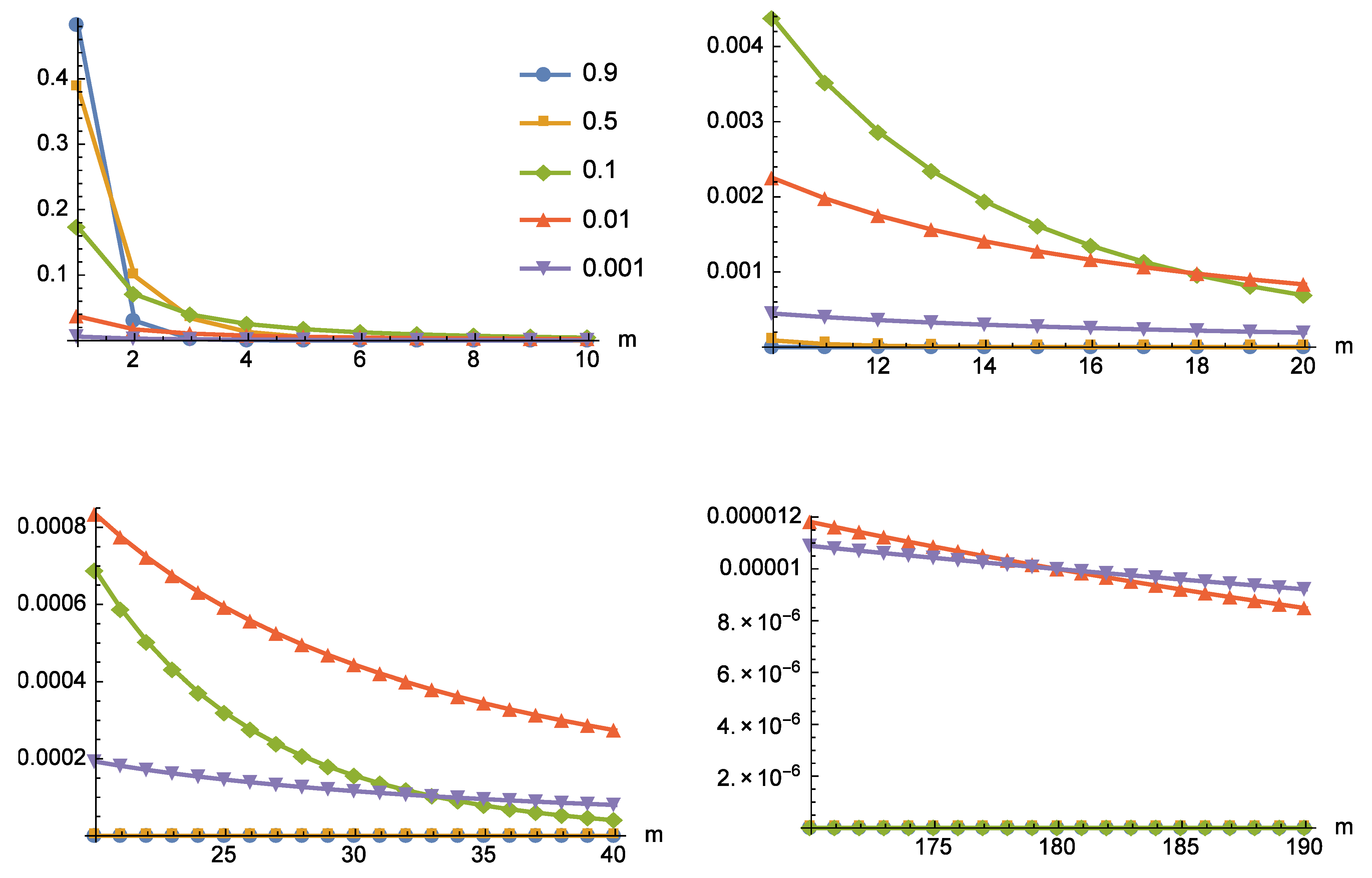
This formula allows a graphic representation of $\mathit{P}\left\{Q=q\right\}$ as a function of the irreducible denominators m displayed in Figure 1, where it is clear how the initial ($m=1$) ordering of the probabilities (increasing with the w values going from $w=0.001$ to $w=0.9$) becomes totally overturned for a large enough m. We remark that each value of the probability (17) should be considered to be attributed to every rational number with the same m as the irreducible denominator. For instance, see Table 2; for $m=1$, we obtain the probability of $q\doteq 0$ and 1; for $m=2$, the probability of $q\doteq {}^1{/}_2$ alone; for $m=3$, that of $q\doteq {}^1{/}_3{,}^2{/}_3$; for $m=4$, that of $q\doteq {}^1{/}_4{,}^3{/}_4;\dots$; and so on. This observation enables us, in particular, to avoid a potential misinterpretation. Indeed, we note that, while it might seem at first glance that

$$\sum _{m=1}^{\infty }\sum _{n=0}^m\mathit{P}\left\{N=n,M=m\right\}=\sum _{m=1}^{\infty }\sum _{n=0}^m\frac{w{(1-w)}^{m-1}}{m+1}=\sum _{m=1}^{\infty }w{(1-w)}^{m-1}=1$$

we find instead

$$\sum _{m=1}^{\infty }\sum _{n=0}^m\frac{w{(1-w)}^{m-1}}{m+1}{}_2{F}_1\left(1,1+{}^1{/}_m;2+{}^1{/}_m;{(1-w)}^m\right)<1$$

as can be seen from the fact that for $0<w<1$

$${}_2{F}_1\left(1,1+{}^1{/}_m;2+{}^1{/}_m;{(1-w)}^m\right)\left\{\begin{array}{cc}=1\hfill & m=1\hfill \\ <1\hfill & m=2,3,\dots \hfill \end{array}\right.$$

This is not in contradiction with the mandatory requirement that

$$\sum _{q\in {\mathbb{Q}}_0}\mathit{P}\left\{Q=q\right\}=1$$

(18)

precisely because, as previously remarked, the probability associated to an m must be attributed to several different rational numbers q; if ${\nu }_m$ is the number of rationals q that have m as its irreducible denominator, then we should rather pay attention to ascertain the normalization in the form

$$\begin{array}{ccc}\hfill \sum _{q\in {\mathbb{Q}}_0}\mathit{P}\left\{Q=q\right\}& =& \sum _{m=1}^{\infty }\sum _{n=0}^m{\nu }_m\frac{w{(1-w)}^{m-1}}{m+1}{}_2{F}_1\left(1,1+{}^1{/}_m;2+{}^1{/}_m;{(1-w)}^m\right)\hfill \\ & =& \sum _{m=1}^{\infty }{\nu }_{m}w{(1-w)}^{m-1}{}_2{F}_1\left(1,1+{}^1{/}_m;2+{}^1{/}_m;{(1-w)}^m\right)=1\hfill \end{array}$$

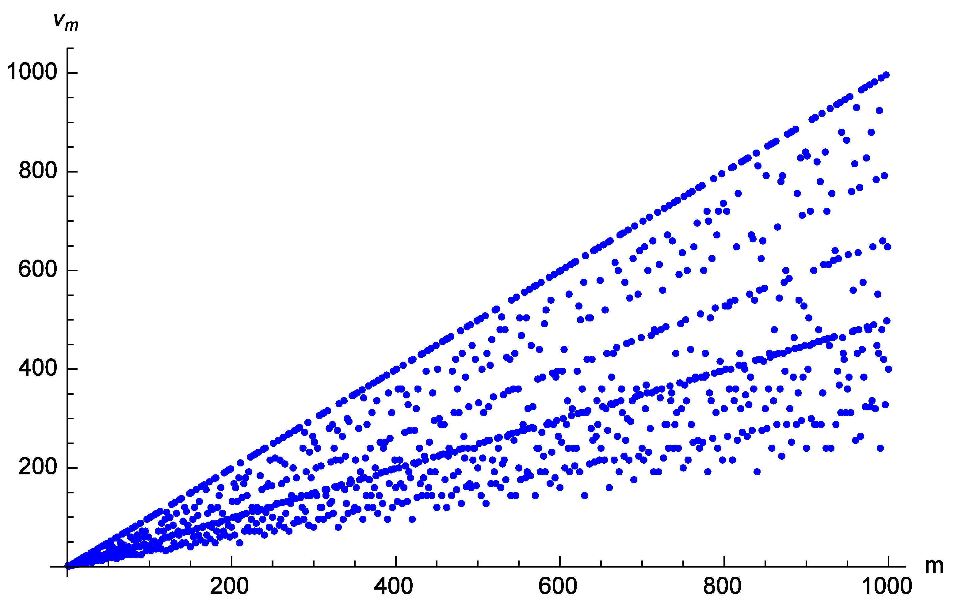
We stress that confirming this result—which we can confidently establish through construction and definition—proves to be challenging when attempting direct calculations. This difficulty arises due to the lack of a readily available closed-form expression for the sequence ${\nu }_m$. The behavior of this sequence is rather irregular, though it demonstrates an overall upward trend on average. This can be observed from an empirical plot of its initial values, depicted in Figure 2. We will defer a more detailed discussion on this matter to Section 7, where we will provide additional insights. In particular, we will demonstrate how the preceding normalization condition can be employed for stepwise computations of the ${\nu }_m$ values.

6.2. Poisson and Equiprobable Denominators

When the denominators are distributed according to different (albeit simple) laws, we no longer have access to elementary closed forms for $\mathit{P}\left\{Q=q\right\}$. For instance, if M follows a Poisson distribution, we have

$$\mathit{P}\left\{M=m\right\}=e^{-\lambda }\frac{{\lambda }^{m-1}}{(m-1)!}\lambda >0,m=1,2,\dots$$

we find $\mathit{E}\left[M\right]=1+\lambda$ and

$$\mathit{E}\left[\frac{1}{M}\right]=\sum _{m=1}^{\infty }\frac{e^{-\lambda }}{m}\frac{{\lambda }^{m-1}}{(m-1)!}=\frac{e^{-\lambda }}{\lambda }\sum _{m=1}^{\infty }\frac{{\lambda }^m}{m!}=\frac{e^{-\lambda }}{\lambda }\left(\sum _{m=0}^{\infty }\frac{{\lambda }^m}{m!}-1\right)=\frac{1-e^{-\lambda }}{\lambda }$$

while for the variance, we have

$$\mathit{V}\left[Q\right]=\frac{1}{12}+\frac{1-e^{-\lambda }}{6\lambda }$$

but the cdf is

$$F_Q\left(x\right)=\left\{\begin{array}{cc}0\hfill & x<0\hfill \\ e^{-\lambda }\sum _{m\ge 1}\frac{{\lambda }^{m-1}}{(m-1)!}\frac{\lfloor mx\rfloor +1}{m+1}\hfill & 0\le x<1\hfill \\ 1\hfill & 1\le x\hfill \end{array}\right.$$

and for the discrete distribution, taking $q\doteq {}^n{/}_m$, we find

$$\mathit{P}\left\{Q=q\right\}=\sum _{\ell =1}^{\infty }\frac{e^{-\lambda }}{\ell m+1}\frac{{\lambda }^{\ell m-1}}{(\ell m-1)!}$$

with no closed expression readily available.

Considering, instead, denominators M taking only a finite number $k=1,2,\dots$ of equiprobable values m, we have:

$$\mathit{P}\left\{M=m\right\}=\left\{\begin{array}{cc}{}^1{/}_k\hfill & m=1,2,\dots ,k\hfill \\ 0\hfill & m>k\hfill \end{array}\right.$$

We then have

$$\mathit{E}\left[M\right]=\frac{k+1}{2}\mathit{E}\left[\frac{1}{M}\right]=\frac{1}{k}\sum _{m=1}^k\frac{1}{m}=\frac{H_k}{k}$$

and, hence,

$$\mathit{V}\left[Q\right]=\frac{1}{12}+\frac{H_k}{6k}$$

while for the cdf it is

$$F_Q\left(x\right)=\frac{1}{k}\sum _{m=1}^k\frac{\lfloor mx\rfloor +1}{m+1}$$

and the discrete distribution probabilities are

$$\mathit{P}\left\{Q=q\right\}=\frac{1}{k}\sum _{\ell =1}^{\lfloor {}^k{/}_m\rfloor }\frac{1}{\ell m+1}q\doteq {}^n{/}_m$$

where, since $m\le k$, it is always $\lfloor {}^k{/}_m\rfloor =1,2,\dots$.

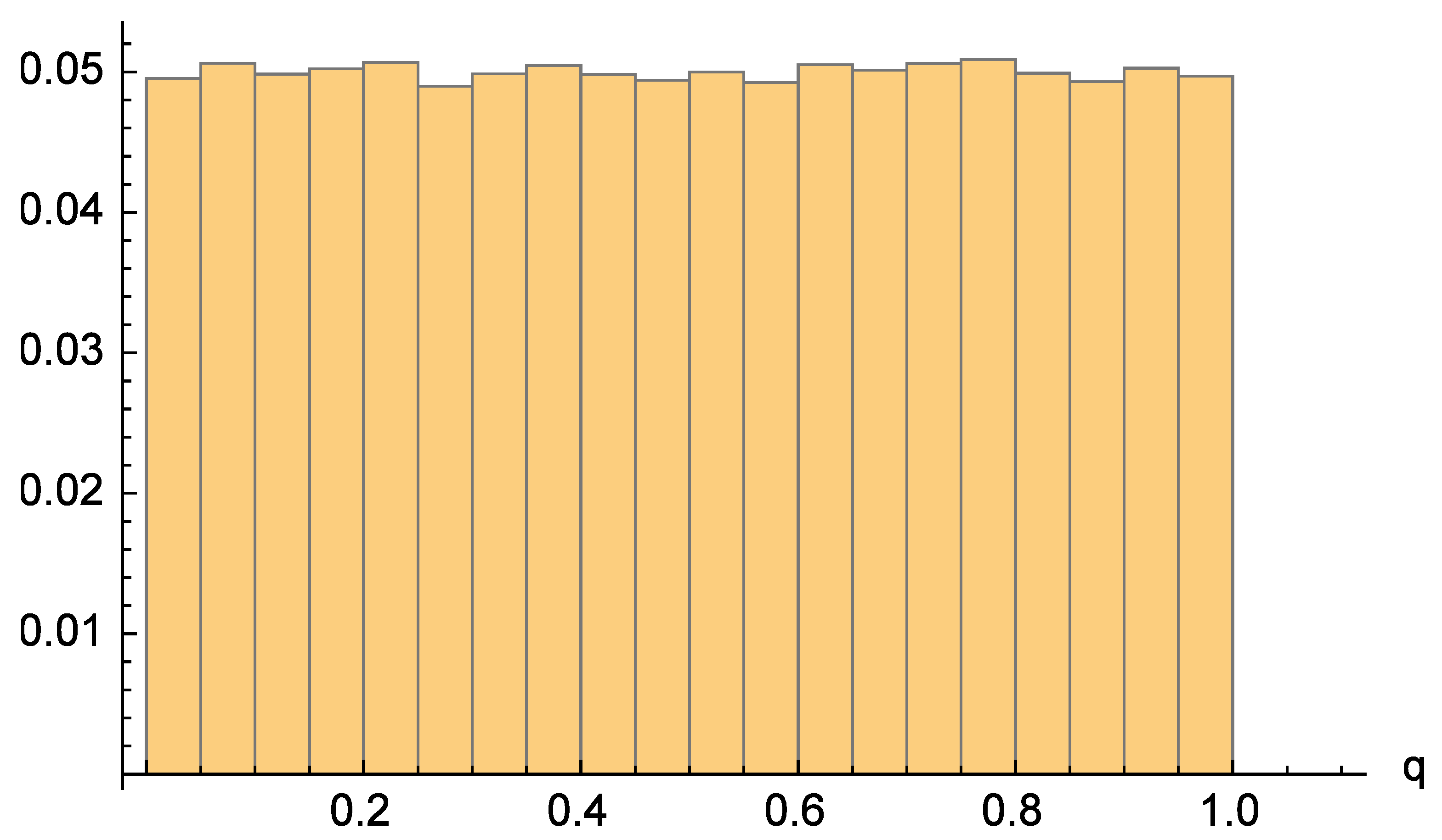
Even in this case, we have no closed formulas to show. Since the sums involved are now always finite, a simple—but essentially trivial—technique for simulating an asymptotically equiprobable sample of rational numbers within the interval $[0,1]$ seems to emerge. The approach involves several steps. Begin by selecting a sufficiently large value k. Then, randomly select an integer m from the equiprobable set of numbers $1,2,\dots ,k$. Subsequently, choose another random integer n from the equiprobable set of numbers $0,1,\dots ,m$, and calculate $q={}^n{/}_m$. By repeating this process a substantial number of times, an almost uniformly distributed sample within the range $[0,1]$ can be generated, as depicted in Figure 3. Nevertheless, it is important to note that the approach has limitations, as mentioned earlier in Section 2. Not every rational number in ${\mathbb{Q}}_0$ would have an opportunity to be drawn using this method, as only a finite subset of these numbers would be taken into account. Although, in theory, this finite set of numbers could be made exactly equiprobable, the infinitely numerous remaining rational numbers would be entirely excluded and assigned a probability of precisely zero.

7. Final Remarks: Sequencing Rational Numbers

Other examples of distributions on the rational numbers in $[0,1]$ are, of course, possible. For instance, given $0<p<1$ and for a given denominator $m=1,2,\dots$, it is possible to suppose that the numerators are binomially—instead of equiprobably—distributed as

$$\mathit{P}\left\{N=n\left|M=m\right.\right\}=\left(\genfrac{}{}{0pt}{}{m}{n}\right)p{(1-p)}^{m-n}n=0,1,\dots ,m$$

By choosing then a suitable distribution for the denominator M, we can define the global distribution of $Q={}^N{/}_M$. However, rather than indulging in displaying these further examples, we would like to conclude this paper with a few remarks about a particular residual open problem.

Due to the countable nature of ${\mathbb{Q}}_0$, as we have already said, its elements within the range $0\le q\le 1$ can be systematically organized into a sequence. To simplify the process of assigning a distribution to ${\mathbb{Q}}_0$, it would be immensely advantageous if this sequence could encompass all rational numbers within $[0,1]$ without any repetitions. Achieving this arrangement, however, requires identifying patterns that govern such sequence. This, in turn, would enable us to easily determine both the rational number q associated with a given index k and, conversely, the index k corresponding to a specific rational number q. Yet, this endeavor is complicated by the inherent irregularity present in the sequence of entries in the triangular table, such as the unpredictable occurrences of prime numbers among the denominators m. Notably, even the presence of prime numbers—which uniquely identify rows without gaps between the extremes—does not follow a readily discernible pattern. Nonetheless, it is evident that effectively sequencing all numbers in ${\mathbb{Q}}_0$ hinges on obtaining insights into ${\nu }_m$—specifically, the count of non-blank entries in the $m^{\mathrm{th}}$ row of

Table 3. Table of rational numbers $q\doteq {}^n{/}_m$ without repetitions, along with the progressive number ${\nu }_m$ of the different rationals sharing a common irreducible denominator m, and their sums ${\sigma }_m$.

								n
${\mathit{\sigma }}_{\mathit{m}}$	${\mathit{\nu }}_{\mathit{m}}$	$\mathit{m}$	$\mathbf{0}$	$\mathbf{1}$	$\mathbf{2}$	$\mathbf{3}$	$\mathbf{4}$	$\mathbf{5}$	$\mathbf{6}$	$\mathbf{7}$	$\mathbf{8}$	$\mathbf{9}$	$\mathbf{10}$
1	2	1	0	1
${}^1{/}_2$	1	2		${}^1{/}_2$
1	2	3		${}^1{/}_3$	${}^2{/}_3$
1	2	4		${}^1{/}_4$		${}^3{/}_4$
2	4	5		${}^1{/}_5$	${}^2{/}_5$	${}^3{/}_5$	${}^4{/}_5$
1	2	6		${}^1{/}_6$				${}^5{/}_6$
3	6	7		${}^1{/}_7$	${}^2{/}_7$	${}^3{/}_7$	${}^4{/}_7$	${}^5{/}_7$	${}^6{/}_7$
2	4	8		${}^1{/}_8$		${}^3{/}_8$		${}^5{/}_8$		${}^7{/}_8$
3	6	9		${}^1{/}_9$	${}^2{/}_9$		${}^4{/}_9$	${}^5{/}_9$		${}^7{/}_9$	${}^8{/}_9$
2	4	10		${}^1{/}_{10}$		${}^3{/}_{10}$				${}^7{/}_{10}$		${}^9{/}_{10}$
5	10	11		${}^1{/}_{11}$	${}^2{/}_{11}$	${}^3{/}_{11}$	${}^4{/}_{11}$	${}^5{/}_{11}$	${}^6{/}_{11}$	${}^7{/}_{11}$	${}^8{/}_{11}$	${}^9{/}_{11}$	${}^{10}{/}_{11}$
⋮	⋮	⋮		⋮									⋮

.

While not attempting an exhaustive treatment of this topic, we will focus on several observations concerning some basic properties of the numbers ${\nu }_m$ (representing the count of rational numbers with a common irreducible denominator m in a row of Table 3) and ${\sigma }_m$ (indicating the sum of these rational numbers). To begin, it is worth noting that the normalization condition (18) can be employed to derive a systematic method for iteratively computing the values of ${\nu }_m$. For example, as detailed in Section 6.1, when denominators follow a geometric distribution and numerators are conditionally equiprobable, the distribution of Q is expressed by (17). To satisfy the normalization (18), the number ${\nu }_m$ of equiprobable numbers sharing the same irreducible denominator must be taken into consideration. It is apparent that by setting $z=1-w$ in (17), the normalization condition (18) transforms into

$$\sum _{q\in {\mathbb{Q}}_0}\mathit{P}\left\{Q=q\right\}=\frac{1-z}{z^2}\sum _{m=1}^{\infty }{\nu }_m\sum _{\ell =1}^{\infty }\frac{z^{m\ell +1}}{m\ell +1}=1$$

namely, with a power expansion

$$\sum _{m=1}^{\infty }{\nu }_m\sum _{\ell =1}^{\infty }\frac{z^{m\ell +1}}{m\ell +1}=\frac{z^2}{1-z}=\sum _{j=0}^{\infty }{z}^{j+2}$$

(19)

This relation can be used to find the values of ${\nu }_m$ by equating the coefficients of the identical powers of z. Indeed, writing the first terms of (19), we find

$$\begin{array}{cc}\hfill & {\nu }_1\left(\frac{z^2}{2}+\frac{z^3}{3}+\frac{z^4}{4}+\frac{z^5}{5}+\dots \right)+{\nu }_2\left(\frac{z^3}{3}+\frac{z^5}{5}+\frac{z^7}{7}+\frac{z^9}{9}+\dots \right)\hfill \\ \hfill & +{\nu }_3\left(\frac{z^4}{4}+\frac{z^7}{7}+\frac{z^{10}}{10}+\frac{z^{13}}{13}+\dots \right)+{\nu }_4\left(\frac{z^5}{5}+\frac{z^9}{9}+\frac{z^{13}}{13}+\frac{z^{17}}{17}+\dots \right)+\dots \hfill \\ \hfill & =z^2+z^3+z^4+z^5+\dots \hfill \end{array}$$

and, hence, we progressively have

$$\begin{array}{ccccc}\hfill & {}^{{\nu }_1}{/}_2=1\hfill & \hfill & \hfill & \hfill {\nu }_1=2\\ \hfill & {}^{{\nu }_1}{/}_3+{}^{{\nu }_2}{/}_3=1\hfill & \hfill & \hfill & \hfill {\nu }_2=1\\ \hfill & {}^{{\nu }_1}{/}_4+{}^{{\nu }_3}{/}_4=1\hfill & \hfill & \hfill & \hfill {\nu }_3=2\\ \hfill & {}^{{\nu }_1}{/}_5+{}^{{\nu }_2}{/}_5+{}^{{\nu }_4}{/}_5=1\hfill & \hfill & \hfill & \hfill {\nu }_4=2\\ \hfill & \dots \hfill & \hfill & \hfill & \hfill \dots \end{array}$$

and so on, in agreement with the corresponding entries of Table 3. It is crucial to emphasize that this procedure cannot rely on the specific distribution of Q since the sequence ${\nu }_m$ remains constant, and the normalization condition (18) must hold for any valid distribution.

To conclude, we will outline a few elementary properties of ${\nu }_m$ and ${\sigma }_m$ that can be instrumental for future advancements. Here, $m=1,2,\dots$ represents the denominators and $n=0,1,\dots ,m$ represents the numerators. We term them accepted when ${}^n{/}_m$ appears in Table 3, meaning it is an irreducible fraction. Here are the properties:

• ${\mathit{\nu }}_{\mathit{m}}\le \mathit{m}-\mathbf{1}$ for $\mathit{m}\ge \mathbf{2}$: in our table $n=0$ and $n=m$ are accepted only for $m=1$ so that, in every row with $m\ge 2$, the first and last number are always missing; then, apparently, ${\nu }_m=(m+1)-2=m-1$; in particular, ${\mathit{\nu }}_{\mathit{m}}=\mathit{m}-\mathbf{1}$ only, for $\mathit{m}$ prime number.
• For $\mathit{m}\ge \mathbf{3}$, if $\mathit{n}=\mathit{k}\ge \mathbf{1}$ is accepted, then $\mathit{n}=\mathit{m}-\mathit{k}\le \mathit{m}-\mathbf{1}$ is also accepted because, if ${}^k{/}_m$ is irreducible, then ${}^{(m-k)}{/}_m=1-{}^k{/}_m$ is also irreducible, namely, the accepted values always show up in pairs; in particular, since $n=1$ is always accepted, then $n=m-1$ is also always accepted, and hence, ${\mathit{\nu }}_{\mathit{m}}\ge \mathbf{2}$ for $\mathit{m}\ge \mathbf{3}$ (the two numbers coincide for $m=2$, so that ${\nu }_2=1$).
• ${\mathit{\nu }}_{\mathit{m}}$ always is an even number for $\mathit{m}\ge \mathbf{3}$ because, according to point 2, the accepted numerators n always show up in pairs; moreover, if $\mathit{m}\ge \mathbf{3}$ is even, then $\mathit{n}={}^{\mathit{m}}{/}_{\mathbf{2}}$ is not accepted because, for $m=2\ell$ (and $\ell \ge 2$), the numerator would be $n={}^m{/}_2=\ell$, and ${}^n{/}_m={}^{\ell }{/}_{2\ell }$ would be a reducible fraction.
• For $\mathit{m}\ge \mathbf{3}$, the sum of an accepted pair always is $\mathbf{1}$ because we are adding ${}^k{/}_m$ and ${}^{(m-k)}{/}_m=1-{}^k{/}_m$; as a consequence, the sum of the irreducible fractions sharing a common denominator $\mathit{m}$ is ${\mathit{\sigma }}_{\mathit{m}}={}^{{\mathit{\nu }}_{\mathit{m}}}{/}_{\mathbf{2}}$ because there are ${}^{{\nu }_m}{/}_2$ accepted pairs; looking, moreover, at Table 3, we see that this last result also holds for $m=1$ (${\nu }_1=2,{\sigma }_1=1$) and $m=2$ (${\nu }_2=1,{\sigma }_2={}^1{/}_2$).

8. Conclusions (Written by Giovanni M. Cicuta)

Let us summarize the findings of this work. The goal of the work is to define a uniform probability distribution to every rational number $q\in [0,1]$. This does not seem to have practical applications today, but it is an intriguing problem. Indeed, it may only be achieved as a limiting process. The main steps are:

For every ratio of pair of random variables $N/M$, with $n\le m$, a uniform distribution for the random variable N is chosen, for fixed m. Next, a sequence, indexed by a parameter k of distributions, is chosen for the random variable M, the denominator.

The k-dependent distribution is increasingly more flat as $k\to \infty$.

In terms of these distributions, a k-dependent probability distribution $\mathit{P}\{Q=q\}$ is defined in Equation (1), for any $q=n/m$, $0\le q\le 1$, where the pair n, m are co-primes. It is defined as asymptotically equiprobable. Theorem 1 asserts that all the desired properties for the probability distribution are achieved through this procedure.

Section 6 provides examples of the distributions for the denominator and detailed evaluations.

Section 7 is not probabilistic. The proof of the countability of rational numbers by G. Cantor provides a sequence of all fractions $n/m$. Several other sequences were written in the decades following this proof. In all of them, every rational number q appears several times (an infinite number of times). One would like to define a sequence of all rational numbers $q\in [0,1]$, such that the sequence of fractions $q=n/m$ would only include the pair n, m as co-primes. In Section 7, some properties of the occurrence of repeated fractions are obtained.

If the desired sequence of rationals numbers without repetitions could be built, many probability distributions could be proposed for the elements of the sequence.