Article

A Computational Fluid Dynamics Study of Flared Gas for Enhanced Oil Recovery Using a Micromodel

by
Stephanie Were
1,
Somtochukwu Godfrey Nnabuife
1,2 and
Boyu Kuang
3,*
1
School of Water, Energy, and Environment, Cranfield University, Cranfield MK43 0AL, UK
2
ODE-Doris Limited, London WC1N 1NN, UK
3
Centre for Computational Engineering Sciences (CES), School of Aerospace, Transport, and Manufacturing, Cranfield University, Cranfield MK43 0AL, UK
*
Author to whom correspondence should be addressed.
AppliedMath 2022, 2(4), 738-757; https://doi.org/10.3390/appliedmath2040044
Submission received: 11 November 2022 / Revised: 3 December 2022 / Accepted: 12 December 2022 / Published: 19 December 2022

Abstract

:
The current handling of gas associated with oil production poses an environmental risk. This gas is being flared off due to the technical and economic attractiveness of this option. As flared gases are mainly composed of methane, they have harmful greenhouse effects when released into the atmosphere. This work discusses the effectiveness of using this gas for enhanced oil recovery (EOR) purposes as an alternative to flaring. In this study, a micromodel was designed with properties similar to a sandstone rock with a porosity of 0.4, and computational fluid dynamics (CFD) techniques were applied to design an EOR system. Temperature effects were not considered in the study, and the simulation was run at atmospheric pressure. Five case studies were carried out with different interfacial tensions between the oil and gas (0.005 N/m, 0.017 N/m, and 0.034 N/m) and different injection rates for the gas (1 × 10⁻³ m/s, 1 × 10⁻⁴ m/s, and 1 × 10⁻⁶ m/s). The model was compared with a laboratory experiment measuring immiscible gas flooding. Factors affecting oil recoveries, such as the interfacial tension between oil and gas, the viscosity, and the pressure, were studied in detail. The results showed that the surface tension between the oil and gas interphase was a limiting factor for maximum oil recovery. The lower surface tension recovered 33% of the original oil in place. The capillary pressure was higher than the pressure in the micromodel, which lowered the amount of oil that was displaced. The study showed the importance of pressure maintenance to increase oil recovery for immiscible gas floods. It is recommended that a wider set of interfacial tensions between oil and gas be tested to obtain a range at which oil recovery is maximum for EOR with flared gas.

1. Introduction

Associated gas, also known as associate petroleum gas (APG), is a combination of gases produced as a by-product of the activities of a crude oil refinery. It is found dissolved in oil or as a gas cap in the oil reservoir. It is common practice to flare off APG during oil production and processing, mainly due to the lack of regulatory policies that prevent the practice as well as the limited level of monitoring. Gas flaring is carried out due to [1] operational safety, which includes unwanted gas diversions or routine gas disposal and venting off to prevent gas build-ups in pipelines, and the cost of flaring being lower than the cost of processing and transporting APG to a suitable market.
APG is mainly composed of natural gas, which can be up to 90% methane and includes smaller amounts of other hydrocarbons. Gas percentages of methane as high as 93% and as low as 7% have been documented [2,3]. The World Bank estimated that about 140 billion cubic meters were flared off in 2018 [4] and initiated the Global Gas Flaring Partnership (GGFP) as an incentive for stakeholders to find alternative uses for flared gas. Figure 1 illustrates the global flaring intensity. Although efforts have been made to lower these figures, countries in Africa, South America, and South Asia exhibit an increase in flaring intensity despite having lower oil production when compared to other countries such as Russia. The high recorded volumes of flared gas provide an opportunity for the development of new markets for the associated gas.
There are many viable solutions to this problem. The production of electricity can be achieved by the use of gas, steam-driven turbines, or reciprocating internal combustion engines [5,6]. Associated gas can be used as a raw material in the production of hydrogen fuel and syngas or for the manufacture of commodities such as rubber, paint, steel, and glass [7,8]. Liquifying associated gas and using it for domestic and industrial purposes also offers a suitable alternative to flaring, although the cost of storage needs to be considered [9]. APG with high concentrations of methane can be used as a substitute for natural gas and used to run natural gas engines [10].
Andres et al. [11] proposed enhanced oil recovery (EOR) as an alternative to flaring off the gas, noting that the definition of EOR has been continuously reviewed in the petroleum industry [12]. The production of oil can be divided into three main stages: primary, secondary, and tertiary extraction. However, there has been a drift from the use of these chronological descriptions, and instead the oil and gas industry tends to refer to these stages as primary, secondary, and EOR [12]. Primary oil recovery occurs when natural reservoir energy displaces oil and gas from a reservoir. As reservoir pressure decreases, artificial lift systems are then implemented. A further decrease in the reservoir pressure results in primary production becoming uneconomical; hence, alternative forms of oil recovery are explored.
Enhanced oil recovery is the terminology used for activities carried out under the secondary and tertiary recovery of oil [13]. Secondary oil extraction activities are mainly water flooding but can include gas injection and pressure maintenance. Tertiary recovery is increasingly energy intensive, comprises activities involving the use of chemicals and thermal energy, and is usually carried out when the secondary recovery process becomes uneconomical.
EOR is one of the main technologies used to maintain oil reserves. It has been reported to recover between 35–50% of the original oil in place (OOIP) [3,4]. Anthropogenic CO2 has historically been used for gas injection, as it simulated oil production while tackling CO2 emissions by carbon sequestration, and it has been documented to have favourable economics [14]. However, its availability is limited, and further research into the use of nitrogen and lean gas (C1) has been conducted [6,7]. The use of flared gas in EOR is still considered unconventional, as more common applications involve setting up full-scale gas processing industries.
Research into the re-injection of gas into a reservoir as an alternative to flaring has been explored, and the economic and environmental merits of this have been considered [11,15]. The re-injection of associated gas for EOR comes with challenges, as a number of interconnected decisions need to be made for it to be successful, and data on the economic implementation are limited to single drill-ready surfaces, which do not reflect realistic systems [16].
Farouq et al. [17] gave an outline of the performance of different EOR methods, with a focus on the mobility ratio and capillary number. A capillary number is a dimensionless group that defines the relationship between the viscous forces and interfacial tension forces that govern fluid flow. A high capillary number is favourable, as it increases oil recovery. The study also highlighted the importance of geological factors and temperature effects in the prediction of oil recovery. They highlighted the different forms in which methane can be used for EOR. These include enriched gas, flu gas, and miscible/immiscible hydrocarbons. The study suggested the use of enriched gas rather than lean gas for better miscibility and higher oil recovery. However, it should be considered that the lower the miscibility, the higher the pressure requirements.
Jin et al. [18] studied WAG flooding with CO2 with a varying composition of methane. Their study showed that miscible oil recovery with methane as an impurity in CO2 could be maintained up to 30 mol%, after which recovery became immiscible. Srivastava et al. [19] conducted laboratory-scale core flood experiments comparing flue gas, APG (75% methane), and CO2 for immiscible gas displacement. In immiscible gas displacement, the viscosity became the most important mechanism for recovery. CO2 outperformed APG in recovery. However, its cost, when compared to APG, was much higher, and its availability was lower than APG. APG outperformed flue gas, giving a better viscosity reduction and higher oil swelling. Yin et al. [20] conducted a similar experiment with higher concentrations of CO2 in APG. They concluded that an increase in CO2 increased recovery, and this could be attributed to the decrease in MMP.
When considering cost, APG outperforms other gases, mainly due to its ready availability, as it is often a by-product of primary recovery. In their review of EOR, Alvarado and Manrique [21] stated that the use of natural gases and associated gas is more economical for offshore fields and fields in remote locations without access to gas markets or gas condensate reservoirs.
APG has also been considered as the gas solvent in WAG injection. These operations are efficient, as they give better volumetric sweeps and fluid displacement. Ahmadi et al. [22] carried out a comprehensive laboratory analysis of continuous and WAG injection methods for heavy oil recovery. APG outperformed water, hot water, CO2, and N2, giving an ultimate recovery of 73%. Through their experiment, they found that the mobility ratio between oil and gas was much lower when compared to the other cases.
Yu et al. [23] carried out experiments injecting natural gas in tight oil reservoirs using the WAG flooding method. From the sensitivity analysis that was conducted, the injection flow rate of the gas played an important role in recovery. Lower gas injection rates were noted to have higher oil recoveries than higher injection rates.
Other than the physical properties of the solvents, Thomas et al. [24] discussed how macro-parameters, including rock geology, heterogeneity, and pressure, and micro-parameters, including gas–fluid interactions and pore size distribution, affect oil recovery and the flooding process. They argued that achieving a perfectly miscible oil recovery was highly improbable, as most solvents will have an IFT with oil that tends to zero rather than a perfect zero. They proposed that a more effective metric when studying oil recovery would be the interactions between the viscosity, IFT, and pore size distribution.
The use of micromodels to study oil properties is now widely accepted to study undiscovered processes and improve the understanding of existing theories [25]. CFD-based micromodels give valuable information on oil recovery systems from miscible/immiscible displacements, flow wettability, capillary effects, and the effects of interfacial tension. The use of micromodels for oil recovery has been reviewed to show the potential of the concept.
Gharibshahi et al. [26] studied the thermal enhanced oil recovery of heavy oil using CFD. They used a 2D micromodel as the porous medium. A random pore distribution network was used for the geometry design based on a glass micromodel used for a similar experiment [27]. The multiphase mixture model was applied to solve equations for the continuity, volume fraction, momentum, and energy; the obtained results were in good agreement with the experimental data.
Zhong et al. [28] used CFD and a micromodel to study two-phase micro-flow water and polymer flooding. They used the volume of fluid (VOF) model to solve for the momentum, continuity, and phase equation of the two-phase interphase. The VOF method, created by Hirts and Nichols [29], was modelled to track the volume fraction of different phases and to approximate the multiphase interphase. For the geometry, they considered an etched pore pattern to reflect the geometric and topological properties of real rocks and built a 2D micromodel from this. The pore network that was formed was complex and reflected the topological features of real rocks, which increased the realism of the simulation.
Hornbrook [30] and Clemens et al. [31] also carried out an etching process to design a micromodel for the study of foam–oil interactions and performed a CFD evaluation of polymer flooding using a micromodel.
The VOF model is widely used to simulate multiphase flow in micromodels. However, it is limited, as it has parasitic velocities, which tends to be the case with all multiphase numerical models. These errors appear as a result of the interface curvature, which is used to calculate the surface tension [32]. The error that is formed is carried forward to the momentum equation; the velocity terms then have to balance these errors, causing spurious velocities. Capillary forces dominate at a microscale, and the bias formed by this phenomenon is increased, compromising the accuracy of the simulation results [33,34].
Doorwar and Mohanty [35] studied viscous fingering on heavy oil recovery using an etched pore pattern micromodel. Viscous fingering is a phenomenon caused by a poor volumetric sweep. It is characterized by a fingered profile formed by the solvent when it bypasses sections within the reservoir that contain oil. The authors carried out water flooding, polymer flooding, and surfactant flooding on the porous media. The observed patterns of viscous fingering were similar to the real nature of viscous fingers.
Ahmadi et al. [36] used a micromodel with a uniform pore network for their study on reservoir heterogeneity and the capillary number. They compared injection well locations using experimental data and data from CFD studies. They concluded that both sets of data agreed.
From the reviewed work, the use of a micromodel in CFD provides valuable insights into injected solvent and oil interactions and the effects on overall oil recovery. Applying field conditions or creating a detailed rock formation in the laboratory is almost impossible. Using CFD in place of experiments on the APG used for gas flooding is less costly and allows for a most precise replication of reservoir conditions. CFD has also been tried, tested, and proven to be a reliable source of data on oil recovery operations, as reviewed above.
Numerical simulation, experimental studies, and theoretical approaches are commonly used to model real-life conditions and to study flow field behaviour. Experiment-based studies are solved using empirical methods, while theoretical methods use the governing equations of fluid mechanics and heat transfer. CFD takes a numerical approach. CFD enables the study of conditions that are difficult or dangerous to achieve in a laboratory, and the scaling up of experimental results is made possible with this tool. It enables the precise collection of data to solve the problem from a flow field model. More importantly, the cost of running CFD calculations is lower than that of an experimental test, which makes it a useful tool for companies trying to create hybrid EOR methods that need to be simulated to check their real-life viability.
This CFD study of flared gas for enhanced oil recovery using a micromodel is divided into three core sections, followed by a conclusion that gives a summary of the findings and future work. In Section 1, a review of the state of non-thermal enhanced oil recovery is presented. The research areas relevant to the objectives are the factors that influence oil recovery by gas flooding and the application of flared gas (APG) in oil recovery as well as experimental studies on enhanced oil recovery using micromodels and CFD. In Section 2, the proposed geometry and simulation parameters are presented. A further investigation into the governing principles of the simulation parameters is conducted. Five case studies to compare the influences of the interfacial tension between the oil and gas and the injection rates of the gas into the reservoir are outlined. In Section 3, the results from the study as well as an in-depth discussion and analysis are presented. Section 4 gives a summary of the work and the conclusions of the study. Areas for further research are discussed.
This paper presents a study on the effectiveness of flared gas for enhanced oil recovery using computational fluid dynamics. The objectives are to design a micromodel geometry for the study and select parameters for the simulation using FLUENT 2019 R2 software, compare the simulated model with experimental data, evaluate the mechanisms that govern the displacement of oil from reservoirs by flared gas, and propose a viable solution for using flared gas for oil recovery. From the analysis, it was found that lowering the surface tension improved oil recovery. However, the accuracy of the results was limited by the effects of numerical dispersions within the simulation when predicting the volumetric flow rates of oil.

2. Methodology

2.1. Geometry

The geometry considered in this CFD study was inspired by Jafari et al. [37], who used a similar geometry for their study on a biosurfactant flooding into a micromodel. Workbench 2019 R2 and Design Modeler were used to create the micromodel, which was the porous medium. The geometry, which was modified for this study, had a random pore network (see Figure 2 (measurement in meters)). The micromodel was modelled in two dimensions (2D) for faster computational speeds.
Taber et al. [38] curated a list of screening criteria for different EOR methods. The recommended porosity for immiscible gas flooding was <0.6. With this in consideration, the geometry was built by randomly distributing 220 circles with different diameters in the domain of the porous medium. Table 1 shows the size distribution of the circles used to form the porous medium. A porosity of 0.4 was obtained by subtracting the surface area of the circles from the main domain. Inlet and outlet ports are displayed on the left and right sides of the geometry, respectively. The dimensions of the model were 21 cm in length and 9 cm in height. The inlet and outlet were each 1 cm long. The model was oriented horizontally to minimize the effects of gravity.

2.2. Mesh Generation

Figure 3 shows the mesh that was used, which was unstructured with triangular cells. Figure 4 shows the mesh from a magnified section of the porous medium. After experimentation, triangular elements were preferred because they gave a better quality mesh around the curves.
A mesh’s element size and type influence the solutions for numerical equations. Therefore, the mesh size selection was important to obtain accurate results. Three meshes with different element sizes were generated. A mesh independence study was conducted to make sure the solutions from the numerical equations were independent of the mesh size. For this study, APG was assumed to flow into the porous medium at a 0.001 m/s velocity with a time step of t = 0.002 s, and the total pressure drop was assessed and used to compare the results of the different meshes that were considered.

2.3. Boundary Conditions

The boundary conditions were set as the velocity inlet and pressure outlet at the inlet and outlet port, respectively. The walls of the porous geometry (the outer walls and the circles) were set as the stationary wall with no slip. In this study, the effects of the contact angle for the gas/oil interphase were neglected for simplicity. At the point of initialization, the porous medium was saturated, with an oil density of 870 kg/m3 and a viscosity of 0.087 kg/ms. An initial gas flooding was conducted at a velocity of 0.001 m/s with a gas density and viscosity calculated to be 0.884 kg/m3 and 1.16142 × 10⁻⁵ kg/ms, respectively [38]. The surface tension for the first case that was investigated was set as 0.034 N/m [39,40]. Simulations were carried out using the Fluent 2019 R2 CFD software.

2.4. Governing Equations

EOR processes are distinctive in character and are based on different reservoir conditions, oil, and injection fluid on the base level. The complexity of the EOR process increases with definitions of solid particles, gas bubble formations, and precipitations [41]. When selecting a multiphase model, these factors therefore need to be considered. Numerous models for analysing multiphase flow are available [42], with some of the more commonly used being the Eulerian mixture and VOF models and the Eulerian–Eulerian model, as presented [43,44].
For this study, the VOF model was selected to investigate the multiphase flow. This model uses momentum equations and the volume fractions of fluids to solve multicomponent systems. The model includes the effects of surface tension for both phases along the cross sections. The equations of volume fraction, continuity, and momentum for microscopic flow using this model [45,46] are provided in Equations (1)–(3):
Volume fraction equation:
q = 1 n a q = 1
Continuity equation:
1 p q [ t ( a q ρ q ) + · ( a q p q v q ) = p = 1 n ( m ˙ p q m ˙ p q ) ]
Momentum equation:
x ( ρ v ) + ( · ρ v v ) = P + · [ μ ( v + v T     ) + ρ g + F ]
Brackbill et al. [47] proposed an equation to model the IFT between the oil and injected fluid interphase, as shown in Equation (4). The equation shows how the VOF model is used to calculate the IFT. The surface force (F) is calculated per unit of interfacial area. It is a function of the curvature of the interphase (k).
F = ( σ K n + σ s ) δ

2.5. Viscous Model

After testing different laminar and turbulence models, the k-omega SST model was selected for the simulation, as it gave the best convergence of residuals when compared to the laminar and standard k-epsilon models. Residuals give the magnitude of error for the governing equations as the iterations progress. The residuals for velocity, k, and omega were <1 × 10⁻⁴, while those of continuity were <1 × 10⁻³, which were within an acceptable range. This model was previously used for porous models with some success [48].

2.6. Solution Methods

The pressure velocity coupling method was selected was coupled. The least-squares cell-based method was used for the gradient, as it has fast computational speeds. The pressure and momentum methods were PRESTO! and second-order upwind, respectfully.

2.7. Case Studies

To determine the effectiveness of APG for EOR using CFD, the most influential factors for immiscible gas recovery had to be analysed. From the review, IFT has the most significant influence on the amount of oil recovered by immiscible gas flooding. Data on IFT values for oil and gas are limited, although the range for oil and gas IFT is between 0 and 0.034 N/m (0.001 N/m=1 dyne/cm). An increase in IFT is an increase in the immiscibility between the oil and gas phases. For APG, standardizing its composition is nearly impossible. By testing a range of IFT values between the oil and gas, information on an optimal range within which APG is most favourable for EOR was obtained. FLUENT software enables the manipulation of IFT values. To test this theory, IFT values of 0.034 N/m, 0.017 N/m, and 0.005 N/m were selected. Table 2 gives a summary of the cases studied. Temperature effects within the micromodel were neglected to simplify the study.
Varying injection rates were also tested to determine if these had an influence on the overall oil recovery. The recommended injection rate is 12 ft/day [49], which is equivalent to 1 × 10⁻⁶ m/s (1 × 10⁻¹¹ m3/s of APG). Three injection rates were tested with the highest immiscibility (0.034 N/m): 1 × 10⁻³ m/s, 1 × 10⁻⁴ m/s, and 1 × 10⁻⁶ m/s.

3. Results

An analysis of the results obtained from the simulations carried out on cases 1–5 was performed. Cases 1–3 were compared regarding the effectiveness and efficiency of oil displacement for immiscible gas flooding. Cases 4 and 5 were used to compare the effect of lowering the injection rate on overall recovery. Running each case on the Cranfield HPC (high-performance computing) system took an average of 10–14 days per case for 300 s worth of data.

3.1. Mesh Independence Study

The results of the mesh independence study are shown in Table 3. The relative error between grids 2 and 3 was larger than that obtained between grids 1 and 2. Grid 1, with 13,950 cells, was chosen to run the simulations, as it appeared that the results obtained with grids 1 and 2 were relatively close, showing some sort of convergence. Grid 1 had a lower number of cells, thus contributing to the lower computational time required for a simulation.

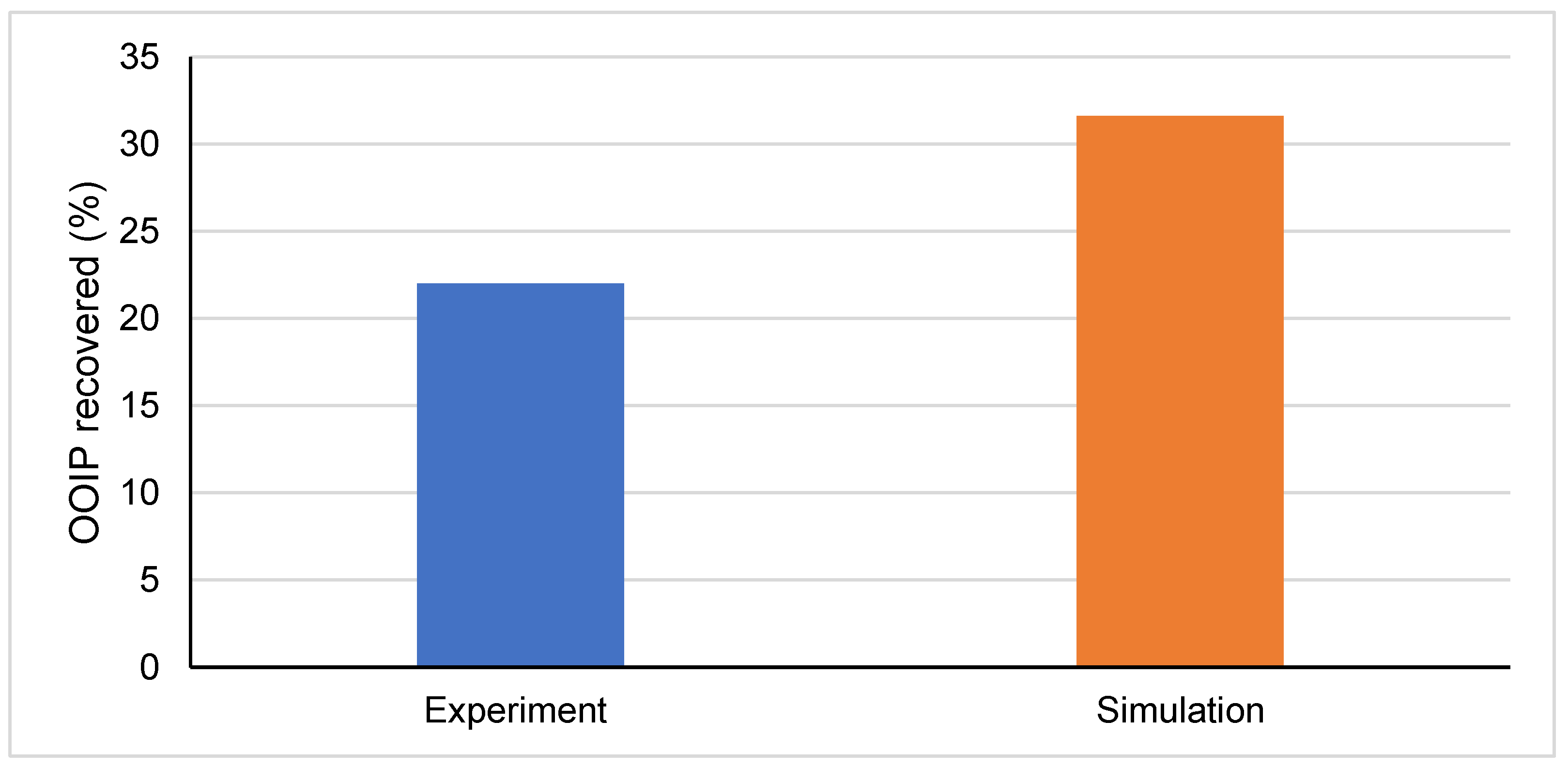
3.2. Model Comparison

To try to check the numerical model, the oil recovery results from the simulation were compared with experimental data [50]. The experiment analysed immiscible gas flooding using air as the gas solvent. Case 1, with an IFT of 0.034 N/m, was selected to compare with the experiment. Air is highly immiscible with oil, which made the comparison with case 1 most appropriate. Both the experiment and the simulation were conducted at atmospheric pressure and neglected temperature effects. Figure 5 shows the comparison of the OOIP recovered from the simulation and the experiment. The simulation had a higher oil displacement (33% of OOIP) than the experiment (22% of OOIP).
The inlet and outlet ports for the model were smaller than that of the simulation, although this did not have an effect on the flow patterns formed by the gas in the porous domain. A study showed that the pore structure significantly affected the effect on the amount of oil displaced, with more uniform and circular pores leading to more oil displacement than pores that were not uniformly structured [51]. Although the shape of the micromodel for the simulation and experiment differed, they both had similar random pore structures, as shown in Figure 6 and Figure 7. However, the porosity for the experimental setup was 0.3, while that of the simulation was 0.4.
Figure 6 and Figure 7 show a comparison of the residual oil from the experiment and simulation at the breakthrough point, respectively. Both models displayed severe gas override and viscous fingering. The experimental setup had more fingered branches due to its lower porosity, which translated to higher capillary forces within the porous domain.

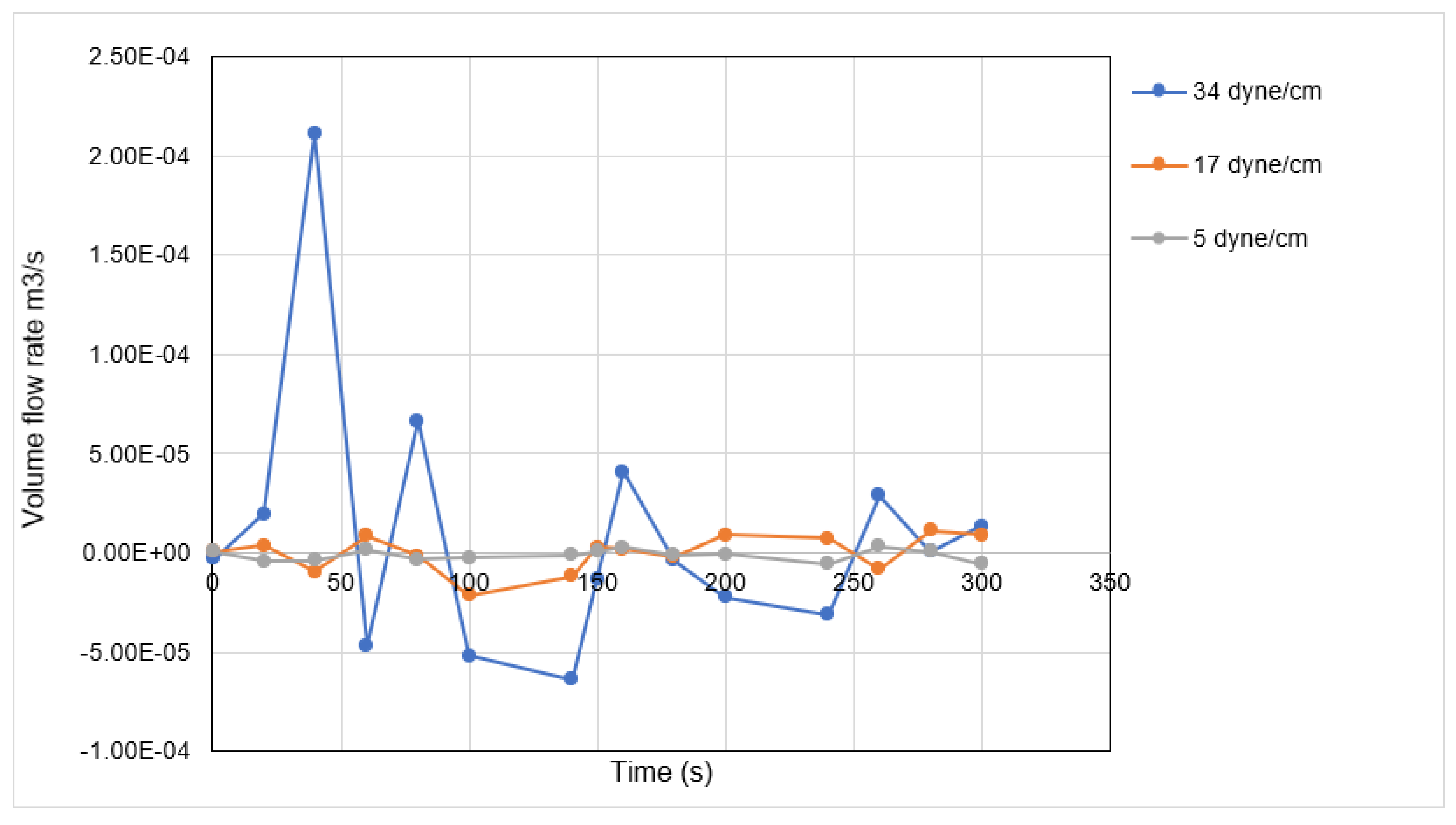
3.3. Inlet Pressure Profile

Figure 8 shows the pressure at which the APG was injected into the micromodel for cases 1, 2, and 3. Along the profile of the micromodel, the inlet pressure decreased for all three cases. At the beginning of the simulation, the pressure was high and dropped sharply as the simulation progressed, levelling off at atmospheric conditions.

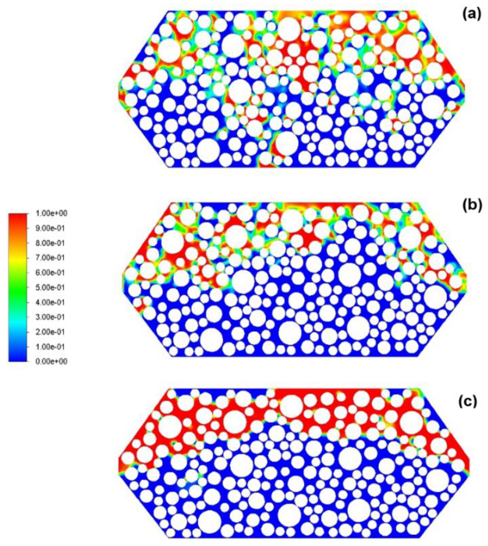
3.4. Oil Displacement

Figure 9 shows the flow of APG in case 1 at different times. The gas phase is represented by the red colour, while the oil phase is blue. A fingering effect was seen almost immediately, as the gas fluid formed a path through the crude oil. From the figure, the breakthrough occurred at 210 s. A breakthrough is defined as a point at which a fluid that was previously isolated from production gains access to a production site or wellbore.
Figure 9 also shows that the gas displacement of the oil on the pore level tended to flow through the larger pores. This is shown clearly in Figure 10, where gas was trapped by the surrounding oil. The narrower pores showed little to no movement of the gas within them. At 300 s, Figure 9 illustrates little breakthrough of APG. At this point, the majority of the oil was trapped in capillaries, and recovery appeared to have reached its peak.
Figure 11 shows a comparison of cases 1–3 at 300s. The colour gradient runs from blue (oil volume fraction at this point is 1) to red (APG volume fraction at this point is 1). Figure 11c displays the smallest amount of trapped oil, with (a) displaying the highest. Figure 11 shows the potential for continued oil recovery where the time for simulation was extended. However, viscous fingering was apparent in all three cases. Less oil entrapment could be attributed to the lower surface tension providing relatively lower immiscible conditions and, consequently, a lower mobility ratio for the oil and gas solvent in Figure 11c when compared to Figure 11a,b.
Figure 12 illustrates the volumetric flow rate for the oil produced in cases 1–3. The volumetric flow profile was not fully developed at 300 s, but from the initial stages it was clear that the surface tension had an effect on the gas fluid flow through the micromodel. At 0.034 N/m, the flow exhibited negative volumes, which could be interpreted as backflows. The volumetric flow at 0.005 N/m experienced little to no resistance and was comparatively the steadiest of the three.
When compared to the oil displacement contours of Figure 11, the volumetric flow profiles show that oil entrapment can cause oscillatory velocities and backflow. This explains the negative volumetric flow rate seen in these cases. A higher IFT caused more resistance to flow within the porous domain. Generally, the volumetric flow of injected APG in the porous medium was low.

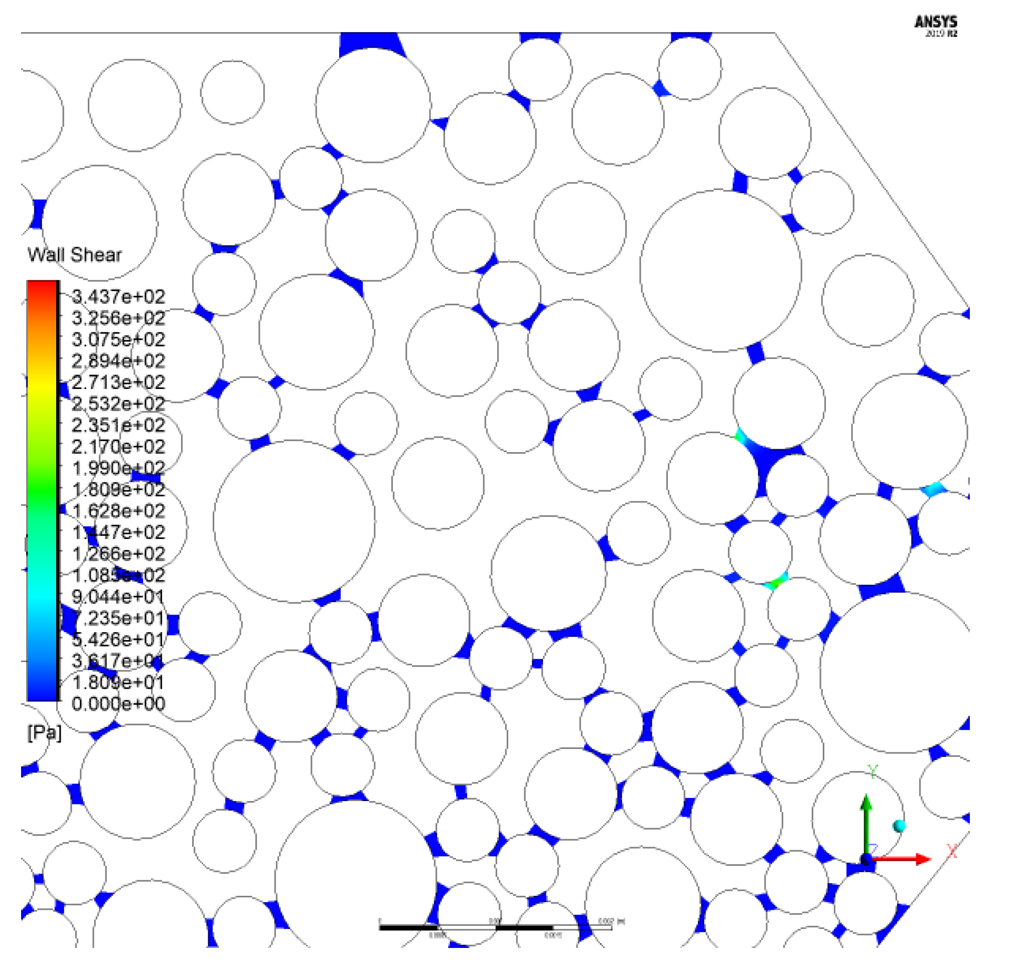
3.5. Pressure and Shear Stress

Figure 13 shows the contours for pressure within the porous domain for case 3. From the figure, the path through which the gas fluid flowed exhibited the lowest pressure. This held true within the domain but not near the walls of the porous medium, which had relatively higher pressure. When compared against the contours of wall shear stress, as seen in Figure 14, the pressure along the walls was identical. The three cases showed identical contours for pressure and shear stress.

3.6. Oil Recovery

The oil recovery is given by the difference between the OOIP and the displaced oil. Figure 15 shows the amount of oil recovered for the different surface tension cases that were simulated. The lower surface tension (case 3) exhibited the highest recovery, while for the higher surface tension (case 1) recovery was significantly lower. Figure 16 shows the trend for oil recovered for cases 1, 2, and 3, with recovery levels of around 30–33% OOIP.
Case 1 (0.034 N/m) appeared to have obtained its upper limit at 30–31% OOIP recovered. However, the recovery profile for case 3 (0.005 N/m) continued to slope upwards. With a longer simulation, it is possible that more oil recovery would have been recorded. For immiscible oil recovery, viscosity played a major role in oil displacement. Figure 17 shows a contour plot for viscosity in the micromodel. The plot illustrates the viscosity reduction action of APG in the porous domain.

3.7. Effect of Injection Fluid Velocity

Table 4 shows the oil recovery for case 1, case 4, and case 5, which had different interjection rates. From the data, there did not seem to be a direct correlation between the injection rate and the amount of oil displaced.

3.8. Discussion

The model comparison was a good indication that the simulation was in line with the expectations from the literature, although it was limiting in that the gas solvent that was used (air) was not the same as APG. The gas that was used and the porosity explained the different fingered profiles between the simulation and experiment. Additionally, the numerical dispersion within the simulation could limit the accuracy of the results.
The inlet pressure for EOR using APG continuously decreased over time. The pressure contours also showed a decrease in pressure within the domain along the path travelled by the gas. For this recovery method to be effective, the data show that external pumping would be required to maintain the reservoir pressure [50]. This has to be put into consideration when selecting an EOR method, as it affects the overall cost of recovery.
Another indication that the system should be pressurized externally was the high volume of oil being trapped within the capillaries. From the results, the narrower pores showed little to no movement of the gas within them; this was theoretically suggested by Chatzis and Dullien [52]. They stipulated that the gas phase displacing the oil interphase breaks through the largest of two pores at a neck. This causes the entrapment of oil in the smaller capillaries. In an immiscible gas injection, capillary forces are dominant within the pores. Capillary pressure resists the entry of gas into pores, and gas pressure cannot easily overcome the capillary barrier and move to the oil phase, enabling displacement. This leads to the entrapment of gas bubbles around the oil. For this to be overcome, the reservoir pressure should exceed the capillary pressure.
The surface tension between the crude oil and the injected gas interphases has a significant impact on oil recovery. Oil recovery with APG injection is immiscible. The interfacial tension for crude oil and various gases has a wide range, depending on the temperature and viscosity (composition) of the oil and the gas composition. This creates a challenge when standardizing the selection of an EOR method for a reservoir. A pilot-scale test must be conducted to ascertain the effectiveness of such an EOR method.
This study on IFT indicates the range within which IFT becomes a limiting factor for maximum oil recovery. From this study, case 3, with an IFT of 0.005 N/m, performed better than cases 1 and 2, which had higher surface tension values; this was in line with the literature. At higher IFT values (cases 1 and 2), oil recovery reached its maximum within 300 s of the simulation. A viscosity reduction within the porous domain is an indicator of a lower IFT between the oil and gas and better oil mobility in these regions.
However, all cases were characterised by common markers that make EOR with immiscible fluids less effective when compared to other EOR methods such as miscible gas flooding.
Immiscible fluids tend to have high mobility ratios (>1). This has an effect on the stability of the oil displacement, which propagates to a poor (volumetric) sweep within the reservoir [53]. From the study, viscous fingering and gas override were observed. Gas override occurs when the injected gas bypasses paths that would lead to oil displacement instead of following a preferential path, mainly due to buoyancy effects. This causes the gas to flow in the upper part of the domain, as was observed in the study. High capillary forces, gas override, and viscous fingering typify immiscible gas injections in EOR.
To improve oil recovery for immiscible gas injections, the natural tendency of injected fluid defaulting to gas overrides (resulting in flows to the producing well directly under gravitational forces), and pressure differentials within the reservoir must be overcome [54]. To accomplish this, the fluid properties that enhance these characteristics and the gravitational effect on the fluid must be mitigated. One solution is to adopt WAG recovery, which has been proven to improve sweep efficiency by lowering immiscible gas mobility ratios, leading to better oil recovery. Hydrocarbon solvent, foam, and polymer injections have also been proven to change the viscosity of the injected fluid, leading to lower mobility ratios.
The injection rate influences the pressure within the micromodel porous domain (reservoir). In the study, however, the effect of the injection rate on the oil recovery was inconclusive. The was no direct effect on oil recovery with an increase or decrease in the gas injection rate. This was possibly because capillary pressure within the domain was a limiting factor to oil recovery for the simulation.
In a particular study, a wide range of gas compositions were tested for immiscible and near-miscible conditions in reservoir conditions [55]. From their analysis, surface tension values as high as 0.0195 N/m and as low as 0.00055 N/m exhibited oil recovery for immiscible conditions. For immiscible injection, the typical oil recovery has been estimated to be less than 60% OOIP [54,56], with some experiments recording oil recoveries as high as 90% [57] and others as low as 22% [50]. The results of the work performed in this study were within range of what has been conducted experimentally on EOR with immiscible gases.
However, macro-parameters that were not considered for this study (such as the rock geology, temperature, and reservoir saturation) need to be considered to conclusively determine the effectiveness of APG for EOR. Although the results were promising, more work needs to be carried out to address the limitations faced in this study.
From the analysis, the viscosity of the fluids is one of the main driving factors for oil recovery by immiscible gas flooding. A lower viscosity for reservoir fluids leads to a better breakthrough, which translates to higher rates of recovery.
Another factor is the capillary pressure. This drives the movement of oil out of the porous domain. Capillary pressure should be kept low/overcome to allow for better recovery.
Lastly, reservoir conditions, which include factors such as the relative permeability, rock formations, and reservoir temperatures, were beyond the scope of this study. These factors, however, play an important role in determining the overall effectiveness of immiscible gas flooding for oil recovery.

4. Conclusions

This paper presented a study on the effectiveness of associated petroleum gas for enhanced oil recovery. The main factor that influences oil recovery for gas injection with APG was identified from the review to be the interfacial tension. Five case studies were carried out with different interfacial tensions between the oil and gas (0.005 N/m, 0.017 N/m, and 0.034 N/m) and different injection rates for the gas (1 × 10⁻³ m/s, 1 × 10⁻⁴ m/s, and 1 × 10⁻⁶ m/s) to test the hypothesis in Section 3. The results obtained for the effect of surface tension were insightful and show promise as a basis for future work.
In summary, a micromodel geometry was first constructed to resemble a sandstone reservoir with a porosity of 0.4. This is within the range of reservoir porosity that is suitable for immiscible gas floods. Second, the simulation of EOR with APG was successfully performed using FLUENT 2019 R2 software. Temperature effects were not considered, and the model was operated at atmospheric pressure for simplification. Third, an analysis of the surface tension effects on EOR showed that it is a limiting factor for maximum oil displacement. The lower surface tension had less oil trapped within the porous domain and better overall oil recovery (33%). Forth, insights from the injection rate and IFT results showed that reservoir pressure maintenance is an important consideration for EOR using APG as the injection fluid because of the high capillary forces seen in the porous medium. Finally, using associate petroleum gas for EOR as an alternative to flaring off the gas can be effective when measures are put in place to improve recovery. The main consideration would be the external pumping required to maintain the reservoir pressure. Alternatively, combining the method with another EOR technique, such as WAG, would reduce the overhead cost of pumping.

5. Future Works

More tests with a wide range of interfacial tensions should be conducted because APG and crude oil compositions are difficult to standardize. This will enable the establishment of a database containing a range of optimal IFT values for maximum oil recovery. Comparative studies with enriched APG under near-miscible conditions (surface tension < 0.001 N/m) should also be conducted. Research comparing near-miscible and miscible gas flooding has provided insightful data on the relevance of first-contact miscibility [54].
A sensitivity analysis on the effects of different concentrations of components that form APG should be conducted. A similar study was carried out on injection gas for EOR [53]. It showed the significance of the injected gas composition on reservoir conditions during oil recovery. A laboratory core flooding experiment with APG under the exact same conditions as in the simulation should be carried out for a more precise validation of the model.
Though oil recovery with APG gas flooding seems feasible, flow assurance considerations such as the effect of reservoir fluid compatibility with the injected gas, gas override due to reservoir heterogeneity, and fingering effects should be assessed before progressing to pilot-scale testing. This will include conducting a test on asphaltene deposition, rock structures, and composition. At a pilot-scale level, the number and positioning of injection wells and production wells will also need to be considered. More elaborate simulations will have to be conducted to ascertain feasibility at this level.

Author Contributions

Conceptualization, S.W. and S.G.N.; methodology, S.W.; software, S.W.; validation, S.W. and S.G.N.; formal analysis, S.W. and S.G.N.; investigation, S.W. and S.G.N.; resources, S.W.; data curation, S.W.; writing—original draft preparation, S.W. and S.G.N.; writing—review and editing, S.W., S.G.N., and B.K.; visualization, S.W. and S.G.N.; supervision, S.G.N. and B.K.; project administration, S.G.N. and B.K. All authors have read and agreed to the published version of the manuscript.

Funding

This research received no external funding.

Institutional Review Board Statement

Not applicable.

Informed Consent Statement

Not applicable.

Data Availability Statement

Not applicable.

Conflicts of Interest

The authors declare no conflict of interest.

Acronyms

APGAssociated Petroleum Gas
CFDComputational Fluid Dynamics
EOREnhanced Oil Recovery
GGFPGlobal Gas Flaring Partnership
IFTInterfacial tension
IRRInternal Rate of Return
VOFVolume of Fluid
OOIPOriginal Oil in Place
RANSReynolds-Averaged Navier–Stokes equation
WAGWater Alternating Gas
MMPMinimum Miscibility Pressure

References

  1. U.S. Department of Energy; Office of Oil and Natural Gas. Natural Gas Flaring and Venting: State and Federal Regulatory Overview, Trends, and Impacts; U.S. Department of Energy: Washington, DC, USA, 2019. [Google Scholar]
  2. Umukoro, G.E.; Ismail, O.S. Modelling Emissions from Natural Gas Flaring. J. King Saud Univ.-Eng. Sci. 2017, 29, 178–182. [Google Scholar] [CrossRef] [Green Version]
  3. Emam, E.A. GAS Flaring in Industry: An Overview. Pet. Coal 2015, 57, 532–555. [Google Scholar]
  4. Bamji, Z. Global Gas Flaring Inches Higher for the First Time in Five Years. Available online: https://blogs.worldbank.org/opendata/global-gas-flaring-inches-higher-first-time-five-years (accessed on 7 June 2020).
  5. Zyryanova, M.M.; Snytnikov, P.V.; Amosov, Y.I.; Belyaev, V.D.; Kireenkov, V.V.; Kuzin, N.A.; Vernikovskaya, M.V.; Kirillov, V.A.; Sobyanin, V.A. Upgrading of Associated Petroleum Gas into Methane-Rich Gas for Power Plant Feeding Applications. Technological and Economic Benefits. Fuel 2013, 108, 282–291. [Google Scholar] [CrossRef]
  6. Rajović, V.; Kiss, F.; Maravić, N.; Bera, O. Environmental Flows and Life Cycle Assessment of Associated Petroleum Gas Utilization via Combined Heat and Power Plants and Heat Boilers at Oil Fields. Energy Convers Manag. 2016, 118, 96–104. [Google Scholar] [CrossRef]
  7. Arutyunov, V.S.; Shmelev, V.M.; Sinev, M.Y.; Shapovalova, O.V. Syngas and Hydrogen Production in a Volumetric Radiant Burner. Chem. Eng. J. 2011, 176–177, 291–294. [Google Scholar] [CrossRef]
  8. Dolinskii, S.E. Economically Attractive Technologies of Deep Conversion of Associated Petroleum Gas. Russ. J. Gen. Chem. 2011, 81, 2574–2593. [Google Scholar] [CrossRef]
  9. Agboola, O.M.; Nwulu, N.I.; Egelioglu, F.; Agboola, O.P. Gas Flaring in Nigeria: Opportunity for Household Cooking Utilization. Int. J. Therm. Environ. Eng. 2010, 2, 69–74. [Google Scholar] [CrossRef]
  10. Gur’yanov, A.I.; Evdokimov, O.A.; Piralishvili, S.A.; Veretennikov, S.V.; Kirichenko, R.E.; Ievlev, D.G. Analysis of the Gas Turbine Engine Combustion Chamber Conversion to Associated Petroleum Gas and Oil. Russ. Aeronaut. 2015, 58, 205–209. [Google Scholar] [CrossRef]
  11. Calderón, A.J.; Pekney, N.J. Optimization of Enhanced Oil Recovery Operations in Unconventional Reservoirs. Appl. Energy 2020, 258, 114072. [Google Scholar] [CrossRef]
  12. Green, D.W.; Willhite, P.G. Enhanced Oil Recovery, 2nd ed.; Society of Petroleum Engineers: Richardson, TX, USA, 1990; ISBN 9781613994948. [Google Scholar]
  13. Ahmadi, M.A.; Shadizadeh, S.R. Nano-Surfactant Flooding in Carbonate Reservoirs: A Mechanistic Study; Springer: Berlin/Heidelberg, Germany, 2017; Volume 132, ISBN 9781555633059. [Google Scholar]
  14. Leach, A.; Mason, C.F.; Van, K. Co-Optimization of Enhanced Oil Recovery and Carbon Sequestration. Resour. Energy Econ. 2011, 33, 893–912. [Google Scholar] [CrossRef] [Green Version]
  15. Jin, L.; Hawthorne, S.; Sorensen, J.; Pekot, L.; Bosshart, N.; Gorecki, C.; Steadman, E.; Harju, J. Utilization of Produced Gas for Improved Oil Recovery and Reduced Emissions from the Bakken Formation. In Proceedings of the Society of Petroleum Engineers-SPE Health, Safety, Security, Environment, and Social Responsibility Conference-North America, Orleans, LA, USA, 18–20 April 2017; pp. 451–458. [Google Scholar]
  16. Hoffman, B.T. Comparison of Various Gases for Enhanced Recovery from Shale Oil Reservoirs. In Proceedings of the Improved Oil Recovery Symposium, Tulsa, OK, USA, 14–18 April 2012; pp. 1–8. [Google Scholar]
  17. Farouq Ali, S.M.; Thomas, S. The Promise and Problems of Enhanced Oil Recovery Methods. J. Can. Pet. Technol. 1996, 35, 57–63. [Google Scholar] [CrossRef]
  18. Jin, L.; Pekot, L.J.; Hawthorne, S.B.; Salako, O.; Peterson, K.J.; Bosshart, N.W.; Jiang, T.; Hamling, J.A.; Gorecki, C.D. Evaluation of Recycle Gas Injection on CO2 Enhanced Oil Recovery and Associated Storage Performance. Int. J. Greenh. Gas Control 2018, 75, 151–161. [Google Scholar] [CrossRef]
  19. Srivastava, R.K.; Huang, S.S.; Dong, M. Comparative Effectiveness of CO2, Produced Gas, and Flue Gas for Enhanced Heavy-Oil Recovery. SPE Reserv. Eval. Eng. 1999, 2, 238–247. [Google Scholar] [CrossRef]
  20. Yin, D.D.; Li, Y.Q.; Zhao, D.F. Utilization of Produced Gas of CO2 Flooding to Improve Oil Recovery. J. Energy Inst. 2014, 87, 289–296. [Google Scholar] [CrossRef]
  21. Alvarado, V.; Manrique, E. Enhanced Oil Recovery: An Update Review. Energies 2010, 3, 1529. [Google Scholar] [CrossRef]
  22. Ahmadi, Y.; Eshraghi, S.E.; Bahrami, P.; Hasanbeygi, M.; Kazemzadeh, Y.; Vahedian, A. Comprehensive Water-Alternating-Gas (WAG) Injection Study to Evaluate the Most Effective Method Based on Heavy Oil Recovery and Asphaltene Precipitation Tests. J. Pet. Sci. Eng. 2015, 133, 123–129. [Google Scholar] [CrossRef]
  23. Yu, H.; Chen, Z.; Lu, X.; Cheng, S.; He, Y.; Shi, L.; Xian, B.; Shi, T. Experimental Study on EOR Performance of Natural Gas Injection in Tight Oil Reservoirs. IOP Conf. Ser. Earth Environ. Sci. 2019, 252, 052021. [Google Scholar] [CrossRef]
  24. Thomas, F.B.; Holowach, N.; Zhou, X.; Bennion, D.B.; Bennion, D.W. SPE/DOE 27811 Miscible or Near-Miscible Gas Injection, Which Is Better? In Proceedings of the SPE/DOE Improved Oil Recovery Symposium, Tulsa, OK, USA, 17–20 April 1994.
  25. Kamari, E.; Rashtchian, D.; Shadizadeh, S.R. Micro-Model Experimental Study of Fracture Geometrical Effect on Breakthrough Time in Miscible Displacement Process. Iran. J. Chem. Chem. Eng. 2011, 30, 1–7. [Google Scholar]
  26. Gharibshahi, R.; Jafari, A.; Ahmadi, H. CFD Investigation of Enhanced Extra-Heavy Oil Recovery Using Metallic Nanoparticles/Steam Injection in a Micromodel with Random Pore Distribution. J. Pet. Sci. Eng. 2019, 174, 374–383. [Google Scholar] [CrossRef]
  27. Sohrabi, M.; Tehrani, D.H.; Danesh, A.; Henderson, G.D. Visualization of Oil Recovery by Water-Alternating-Gas Injection Using High-Pressure Micromodels. SPE J. 2004, 9, 290–301. [Google Scholar] [CrossRef]
  28. Zhong, H.; Li, Y.; Zhang, W.; Li, D. Study on Microscopic Flow Mechanism of Polymer Flooding. Arab. J. Geosci. 2019, 12, 56. [Google Scholar] [CrossRef]
  29. Hirt, C.W.; Nichols, B.D. Volume of Fluid (VOF) Method for the Dynamics of Free Boundaries. J. Comput. Phys. 1981, 39, 201–225. [Google Scholar] [CrossRef]
  30. Hornbrook, J.W.; CastaJnier, L.M.; Pettit, P.A. Observation of Foam/Oil Interactions in a New, High-Resolution Micromodel. In Proceedings of the 66th Annual Technical Conference and Exibition of the Society of Petroleum Engineers, Dallas, TX, USA, 6–9 October 1991; pp. 377–382. [Google Scholar]
  31. Clemens, T.; Tsikouris, K.; Buchgraber, M.; Castanier, L.; Kovscek, A. Pore-Scale Evaluation of Polymers Displacing Viscous Oil-Computational- Fluid-Dynamics Simulation of Micromodel Experiments. SPE Reserv. Eval. Eng. 2013, 16, 144–154. [Google Scholar] [CrossRef]
  32. Renardy, Y.; Renardy, M. PROST: A Parabolic Reconstruction of Surface Tension for the Volume-of-Fluid Method. J. Comput. Phys. 2002, 183, 400–421. [Google Scholar] [CrossRef] [Green Version]
  33. Raeini, A.Q.; Blunt, M.J.; Bijeljic, B. Modelling Two-Phase Flow in Porous Media at the Pore Scale Using the Volume-of-Fluid Method. J. Comput. Phys. 2012, 231, 5653–5668. [Google Scholar] [CrossRef]
  34. Soh, G.Y.; Yeoh, G.H.; Timchenko, V. A CFD Model for the Coupling of Multiphase, Multicomponent and Mass Transfer Physics for Micro-Scale Simulations. Int. J. Heat Mass Transf. 2017, 113, 922–934. [Google Scholar] [CrossRef] [Green Version]
  35. Doorwar, S.; Mohanty, K.K. Viscous Fingering during Non-Thermal Heavy Oil Recovery. In Proceedings of the SPE 146841-MS, Proceedings of the SPE Annual Technical Conference and Exibition, Denver, CO, USA, 30 October–2 November 2011. [Google Scholar]
  36. Ahmadi, P.; Ghandi, E.; Riazi, M.; Malayeri, M.R. Experimental and CFD Studies on Determination of Injection and Production Wells Location Considering Reservoir Heterogeneity and Capillary Number. Oil Gas Sci. Technol. 2019, 74, 4. [Google Scholar] [CrossRef] [Green Version]
  37. Jafari, A.; Pour, S.E.F.; Gharibshahi, R. CFD Simulation of Biosurfactant Flooding into a Micromodel for Enhancing the Oil Recovery. Int. J. Chem. Eng. Appl. 2016, 7, 353–358. [Google Scholar] [CrossRef] [Green Version]
  38. UNITROVE Natural Gas Density Calculator. Available online: https://www.unitrove.com/engineering/tools/gas/natural-gas-density (accessed on 4 June 2020).
  39. Watts, D. Interfacial Tension. Available online: https://petrowiki.org/Interfacial_tension (accessed on 14 December 2022).
  40. Dalvand, K.; Heydarian, A. Determination of Gas-Oil Interfacial Tension. Energy Sources Part A Recovery Util. Environ. Eff. 2015, 37, 1790–1796. [Google Scholar] [CrossRef]
  41. Wu, Y.S. Multiphase Fluid Flow in Porous and Fractured Reservoirs; Gulf Professional Publishing: Houston, TX, USA, 2015; ISBN 9780128038482. [Google Scholar]
  42. Chen, Z.; Huan, G.; Ma, Y. Computational Methods for Multiphase Flows in Porous Media; Society for Industrial and Applied Mathematics: Philadelphia, PA, USA, 2006; Volume 2, ISBN 0898716063. [Google Scholar]
  43. Ferziger, J.H.; Peric, M. Computational Methods for Fluid Dynamics, 3rd ed.; Springer International Publishing: Stanford, CA, USA, 2002; ISBN 3540420746. [Google Scholar]
  44. Shahmohammadi, A.; Jafari, A. Application of Different CFD Multiphase Models to Investigate Effects of Baffles and Nanoparticles on Heat Transfer Enhancement. Front. Chem. Sci. Eng. 2014, 8, 320–329. [Google Scholar] [CrossRef]
  45. Chung, T.J. Computational Fluid Dynamics, 2nd ed.; Cambridge University Press: Cambridge, UK, 2002; ISBN 9780521595353. [Google Scholar]
  46. Jafari, A.; Hasani, M.; Hosseini, M.; Gharibshahi, R. Application of CFD Technique to Simulate Enhanced Oil Recovery Processes: Current Status and Future Opportunities. Pet. Sci. 2020, 17, 434–456. [Google Scholar] [CrossRef] [Green Version]
  47. Brackbill, J.U.; Kothe, D.B.; Zemach, C. A Continuum Method for Modeling Surface Tension. J. Comput. Phys. 1992, 100, 335–354. [Google Scholar] [CrossRef]
  48. Wood, B.D.; He, X.; Apte, S.V. Modeling Turbulent Flows in Porous Media. Annu. Rev. Fluid Mech. 2020, 52, 171–203. [Google Scholar] [CrossRef] [Green Version]
  49. Meybodi, H.E.; Kharrat, R.; Ghazanfari, M.H. Effect of Heterogeneity of Layered Reservoirs on Polymer Flooding: An Experimental Approach Using Five-Spot Glass Micromodel. In Proceedings of the 2008 SPE Europec/EAGE Annual Conference and Exibition, Rome, Italy, 9–12 June 2008. [Google Scholar]
  50. Hauhs, F.; Födisch, H.; Hincapie, R.E.; Ganzer, L. Novel Evaluation of Foam and Immiscible Gas Flooding in Glass-Silicon-Glass Micromodels. In Proceedings of the 80th EAGE Conference and Exhibition, Copenhagen, Denmark, 11–14 June 2018. [Google Scholar]
  51. Gharibshahi, R.; Jafari, A.; Haghtalab, A.; Karambeigi, M.S. Application of CFD to Evaluate the Pore Morphology Effect on Nanofluid Flooding for Enhanced Oil Recovery. RSC Adv. 2015, 5, 28938–28949. [Google Scholar] [CrossRef]
  52. Chatzis, I.; Dullien, F.A.L. Dynamic Immiscible Displacement Mechanisms in Pore Doublets: Theory versus Experiment. J. Colloid Interface Sci. 1983, 91, 199–222. [Google Scholar] [CrossRef]
  53. Mohammadi, S.; Khalili, M.; Mehranfar, M. The Optimal Conditions for the Immiscible Gas Injection Process: A Simulation Study. Pet. Sci. Technol. 2014, 32, 225–239. [Google Scholar] [CrossRef]
  54. Sohrabi, M.; Danesh, A.; Tehrani, D.H.; Jamiolahmady, M. Microscopic Mechanisms of Oil Recovery by Near-Miscible Gas Injection. Transp. Porous Media 2008, 72, 351–367. [Google Scholar] [CrossRef]
  55. Firoozabadi, A.; Katz, D.L.; Soroosh, H.; Sajjadian, V.A. Surface Tension of Reservoir Crude-Oil/Gas Systems Recognizing the Asphalt in the Heavy Fraction. SPE Reserv. Eng. (Soc. Pet. Eng.) 1988, 3, 265. [Google Scholar] [CrossRef]
  56. Shariatpanahi, S.F.; Dastyari, A.; Bashukooh, B.; Haghighi, M.; Sahimi, M.; Ayatollahi, S.S. Visualization Experiments on Immiscible Gas and Water Injection by Using 2D-Fractured Glass Micromodels. In Proceedings of the 14 th SPE Middle East Oil and Gas Show and Conference, Manama, Bahrain, 12–15 March 2005; pp. 907–915. [Google Scholar]
  57. Danesh, A.; Krinis, D.; Henderson, G.D.; Peden, J.M. Pore-Level Visual Investigation of Miscible and Immiscible Displacements. J. Pet. Sci. Eng. 1989, 2, 167–177. [Google Scholar] [CrossRef]
Figure 1. Flaring intensity (m3/barrel). Source: NOAA/GGFFR.
Appliedmath 02 00044 g001
Figure 2. The geometry of the micromodel that was considered.
Appliedmath 02 00044 g002
Figure 3. Mesh generated for this study.
Appliedmath 02 00044 g003
Figure 4. A closer view of the mesh built with triangular cells.
Appliedmath 02 00044 g004
Figure 5. Comparison of OOIP recovered from the simulation and experiment.
Appliedmath 02 00044 g005
Figure 6. The volume fraction of residual oil (green) from the experiment after breakthrough.
Appliedmath 02 00044 g006
Figure 7. The volume fraction of residual oil (blue) from the simulation after breakthrough.
Appliedmath 02 00044 g007
Figure 8. Inlet pressure of injected APG against time.
Appliedmath 02 00044 g008
Figure 9. Volume fraction of oil displaced (blue) at different times by injected APG (red) for case 1.
Appliedmath 02 00044 g009
Figure 10. Trapped oil (blue) in the micromodel.
Appliedmath 02 00044 g010
Figure 11. Comparison of oil displaced at 300 s for (a) 0.034 N/m (case 1), (b) 0.017 N/m (case 2), and (c) 0.005 N/m (case 3). The blue region represents the volume fraction of oil, and the red represents the volume fraction of APG.
Appliedmath 02 00044 g011
Figure 12. Volumetric flow rate of oil produced against time for case 1, case 2, and case 3. The flow for case 1 (0.034 N/m) was characterised by negative volumes.
Appliedmath 02 00044 g012
Figure 13. Contours of pressure for case 3 at 300 s.
Appliedmath 02 00044 g013
Figure 14. Contour of wall shear stress for case 3 at 300 s.
Appliedmath 02 00044 g014
Figure 15. Oil recovered as a percentage of OOIP.
Appliedmath 02 00044 g015
Figure 16. Effect of surface tension on oil recovery.
Appliedmath 02 00044 g016
Figure 17. Contours of viscosity for case 1 at 300 s.
Appliedmath 02 00044 g017
Table 1. Circle diameters and quantities.
Diameter (mm)NumberPercentage Area (%)
1.41035
1.01935
0.86915
0.612415
Table 2. Summary of cases studied.
Case No.IFT (N/m)Gas Injection Velocity (m/s)
10.0341 × 10⁻³
20.0171 × 10⁻³
30.0051 × 10⁻³
40.0341 × 10⁻⁴
50.0341 × 10⁻⁶
Table 3. Mesh independence.
Grid No.No. of CellsDP (Pa)Relative Error (%)
Grid 113,9500.22764.6573
Grid 217,2170.2382
5.2477
Grid 342,2100.2507
Table 4. Oil recovery for different injection rates.
Case No.Injection Rate (m/s)Oil Recovery (% OOIP)
Case 11 × 10−331.6
Case 41 × 10−427.3
Case 51 × 10−629.9
Publisher’s Note: MDPI stays neutral with regard to jurisdictional claims in published maps and institutional affiliations.

