Chaotic Behavior of the Zakharov-Kuznetsov Equation with Dual-Power Law and Triple-Power Law Nonlinearity

Abstract

The main idea of this paper is to study the chaotic behavior of Zakharov–Kuznetsov equation with perturbation. By taking the traveling wave transformation, we transform the perturbed Zakharov–Kuznetsov equation with dual-power law and triple-power law nonlinearity into planar dynamic systems, and then analyze how the external perturbed terms affect the chaotic behavior. We emphasize here that there is no chaotic phenomenon for the non-perturbed ZK equation, thus it is only caused by the external perturbed terms.

1. Introduction

The Zakharov–Kuznetsov (ZK) equation plays an important role in modeling weakly nonlinear ion-acoustic waves in a plasma [1,2,3], and has been yet studied by many researchers and a lot of valuable results have been obtained. For example, Wazwaz studied this equation and obtained the soliton and periodic solutions [4]. Other progress about this equation could be seen in [5,6].

Recently, the ZK equation in its modified form has attracted a lot attention due to its wide applications in weakly nonlinear ion-acoustic modes with strongly magnetized plasma, and its general form could be written as

$$u_t+G\left(u\right)u_x+\sigma {(u_{xx}+u_{yy})}_x=0,$$

(1)

where $G\left(u\right)$ is a differentiable function and $\sigma$ is a real constant. When $G\left(u\right)=u^{1/2}$, the corresponding equation of (1) is derived by Schamel [7] to study ion-acoustic waves due to resonant electrons. In order to promote this equation into a wider field of application, other forms of this equation, such as the ZK equation with power-law nonlinearity and dual-power law nonlinearity, are also derived [8,9].

In this paper, we consider the following ZK equation with dual-power law nonlinearity

$$u_t+(a{u}^n+b{u}^{2n})u_x+\sigma {(u_{xx}+u_{yy})}_x=r_1(x,t),$$

(2)

and triple-power law nonlinearity

$$u_t+(a{u}^n+b{u}^{2n}+c{u}^{3n})u_x+\sigma {(u_{xx}+u_{yy})}_x=r_2(x,t),$$

(3)

where $a,b$ and c are all real constants and $r_i(x,y,t)(i=1,2)$ are the corresponding external perturbed terms. Equation (2) could be treated similarly as (3) by setting $c=0$. We analyze the chaotic behavior of (2) and (3) with the variation of the parameters $a,b$ and c when the perturbed terms are in the special form of $r(x,t)=r(x+y-lt)$. The unperturbed form of (2) is solved by Biswas and Zerrad [9] and a one-soliton solution is obtained. Other recent progress about ZK equation could be seen [10,11].

Chaotic motion is usually observed in the high order dynamic systems. However, recently, Yin and her colleagues studied the chaotic phenomena of the Schrödinger equation with the power-law nonlinearity when the power exponent is fractional via the qualitative theory of planar dynamic system [12]. Their findings are surprising, and the link of chaotic motion with perturbed terms is established. In this paper, we show that when the power exponent is an integer and the perturbed terms are in other forms, the chaotic phenomena are also present in (2) and (3).

This paper is organized as follows. In Section 2, the traveling wave transformation is applied to (2) and (3) with no perturbed term and the corresponding traveling wave systems are obtained, then the Hamiltonians are constructed via it. Moreover, the qualitative analysis to the corresponding dynamic system is conducted. In Section 3, we show the chaotic motion with two kinds of external perturbed terms. The Lyapunov exponents and the corresponding global phase portraits are given to show the chaotic behaviors. In the final, a short conclusion is given.

2. Qualitative Analysis for ZK Equation

In this section, we obtain the dynamic system and Hamiltonian of ZK equation by taking the traveling wave transformation. The qualitative analysis are conducted to obtain the existence of solitons and periodic solutions. Moreover, we also show corresponding phase diagrams, which allows us to see the form of the solutions more clearly.

2.1. ZK Equation with Dual-Power Law Nonlinearity

By taking the following transformation

$$\xi =x+y-lt,$$

(4)

where l is the velocity of the wave, then Equation (2) becomes

$$-l{u}^{\prime }+(a{u}^n+b{u}^{2n})u^{\prime }+2\sigma u^{‴}=r_1\left(\xi \right).$$

(5)

Integrating it once yields

$$-lu+\frac{a}{n+1}{u}^{n+1}+\frac{b}{2n+1}{u}^{2n+1}+2\sigma u^{″}=R_1\left(\xi \right),$$

(6)

where $R_1\left(\xi \right)=\int r_1\left(\xi \right)d\xi$.

(6) is equivalent to the following dynamic system

$$\left\{\begin{array}{c}{u}^{\prime }=v,\hfill \\ v^{\prime }=\frac{1}{2\sigma }[a_1{u}^{n+1}+a_2{u}^{2n+1}+a_{3}u+R_1\left(\xi \right)],\hfill \end{array}\right.$$

(7)

where $a_1=-\frac{a}{n+1},a_2=-\frac{b}{2n+1}$ and $a_3=l$. In the following, we first consider the non-perturbed condition, namely $R_1\left(\xi \right)=0$. Then (6) becomes

$$-lu+\frac{a}{n+1}{u}^{n+1}+\frac{b}{2n+1}{u}^{2n+1}+2\sigma u^{″}=0.$$

(8)

Integrating it once, we have

$$-\frac{l}{2}{u}^2+\frac{a}{(n+1)(n+2)}{u}^{n+2}+\frac{b}{(2n+1)(2n+2)}{u}^{2n+2}+\sigma u^{\prime 2}=c,$$

(9)

where c is a constant of integration. Via (9), we can obtain a conserved quantity

$$H=\frac{v^2}{2}-\frac{l}{2\sigma }{u}^2+\frac{a}{(n+1)(n+2)\sigma }{u}^{n+2}+\frac{b}{(2n+1)(2n+2)\sigma }{u}^{2n+2},$$

(10)

where v is the generalized momentum. It is easy to verify the following formula

$$\left\{\begin{array}{c}\frac{\partial H}{\partial \xi }=0,\hfill \\ \frac{\partial H}{\partial v}=u^{\prime },\frac{\partial H}{\partial u}=-v^{\prime },\hfill \end{array}\right.$$

(11)

thus H is a Hamiltonian and it represents a constant motion for $\frac{\partial H}{\partial \xi }=0$. Moreover, in this non-perturbed case, (7) becomes

$$\left\{\begin{array}{c}{u}^{\prime }=v,\hfill \\ v^{\prime }=u(A{u}^{2n}+B{u}^n+C)=uf\left(u\right),\hfill \end{array}\right.$$

(12)

where $A=\frac{a_2}{2\sigma },B=\frac{a_2}{2\sigma }$, $C=\frac{a_3}{2\sigma }$ and $f\left(u\right)=A{u}^{2n}+B{u}^n+C$. By introducing the following discriminant

$$\mathsf{\Delta }=B^2-4AC,$$

(13)

we can see that three cases need to be discussed here. We have to emphasize here that we only focus on the condition that n is odd, and other conditions could be treated similarly.

Case 1. When $\mathsf{\Delta }>0$, we have

$$f\left(u\right)=A(u^n-s_1)(u^n-s_2),(s_1>s_2)$$

(14)

then the system (12) has three equilibrium points $P_1=(0,0),P_2=(s_1^{1/n},0)$ and $P_3=(s_2^{1/n},0)$. When $A>0$, $P_1$ is a center and $P_2$ and $P_3$ are two saddle points, whereas when $A<0$, $P_1$ is a saddle point and $P_2$ and $P_3$ are two centers. For example, when $n=3$, $s_1=1$, $s_2=-1$ and $A=\pm 8$, the corresponding global phase portraits are given in Figure 1.

We can conclude from Figure 1 that when $A>0$, the original equation has kink soliton and periodic solution. When $A<0$, it has bell-shaped soliton and periodic solution [13].

Case 2. When $\mathsf{\Delta }=0$, we have

$$f\left(u\right)=A{(u^n-s)}^2,$$

(15)

then the system (12) has two equilibrium points $P_1=(0,0),P_2=(s^{1/n},0)$, where $P_2$ is a cuspidal point. When $A>0$, $P_1$ is a saddle point and when $A<0$, $P_1$ is a center. For example, when $s=1,n=3$ and $A=\pm 8$, the corresponding global phase portraits are given in Figure 2.

We can conclude from Figure 2 that when $A>0$, the original equation has a kink soliton and periodic solution. When $A<0$, it has a bell-shaped soliton and periodic solution.

Case 3. When $\mathsf{\Delta }<0$, we have

$$f\left(u\right)=A{(u^n-s_1)}^2+s_2^2,$$

(16)

this case is similar to Case 1, so concrete discussion is omitted. From the basic theory of bifurcation method, we can see that Equation (5) has periodic and bell-shaped soliton solution [13,14], and it is also easy to see that there is no chaotic behavior discovered here. In the next section, we continue to solve ZK equation with dual-power law nonlinearity.

2.2. ZK Equation with Triple-Power Law Nonlinearity

By the traveling wave transformation $\xi =x+y-lt$ and integrating (3), we have

$$-lu+\frac{a}{n+1}{u}^{n+1}+\frac{b}{2n+1}{u}^{2n+1}+\frac{c}{3n+1}{u}^{3n+1}+2\sigma u^{″}=R_2\left(\xi \right),$$

(17)

where $R_2\left(\xi \right)=\int r_2\left(\xi \right)d\xi$. (17) is equivalent to the following dynamic system

$$\left\{\begin{array}{c}{u}^{\prime }=v,\hfill \\ v^{\prime }=\frac{1}{2\sigma }[b_1{u}^{n+1}+b_2{u}^{2n+1}+b_3{u}^{3n+1}+b_4{u}^2+R_2\left(\xi \right)],\hfill \end{array}\right.$$

(18)

where $b_1=-\frac{a}{n+1},b_2=-\frac{b}{2n+1},b_3=-\frac{c}{3n+1}{u}^{3n+1}$ and $b_4=l$. Via (18), a conserved quantity could be constructed as follows

$$\begin{array}{cc}\hfill & H=\frac{v^2}{2}-\frac{l}{2\sigma }{u}^2+\frac{a}{(n+1)(n+2)\sigma }{u}^{n+2}\hfill \\ \hfill & +\frac{b}{(2n+1)(2n+2)\sigma }{u}^{2n+2}+\frac{c}{(3n+1)(3n+2)\sigma }{u}^{3n+2}.\hfill \end{array}$$

(19)

It is easy to verify that (19) is also a Hamiltonian. Via the same procedure, we can obtain the dynamic properties of Equation (18) such as equilibrium points, global phase portraits and existences of soliton and periodic solutions. We do not intend to show these results here, and you can refer to Refs. [13,14] for concrete discussions.

This section deals with (2) and (3) in unperturbed form, and some dynamic properties are presented. In the next section, we will analyze the chaotic motion of their perturbed form. With the variation of the parameters and the perturbed terms, we can see that intensity of the chaotic behavior also changes.

3. The Chaotic Motions

We conduct the qualitative analysis to the ZK equation in the non-perturbed case and find that there is no chaotic phenomenon under the traveling wave structure. Considering the dynamic system (7) and (18), we can actually obtain different chaotic motions with the variation of the perturbed terms.

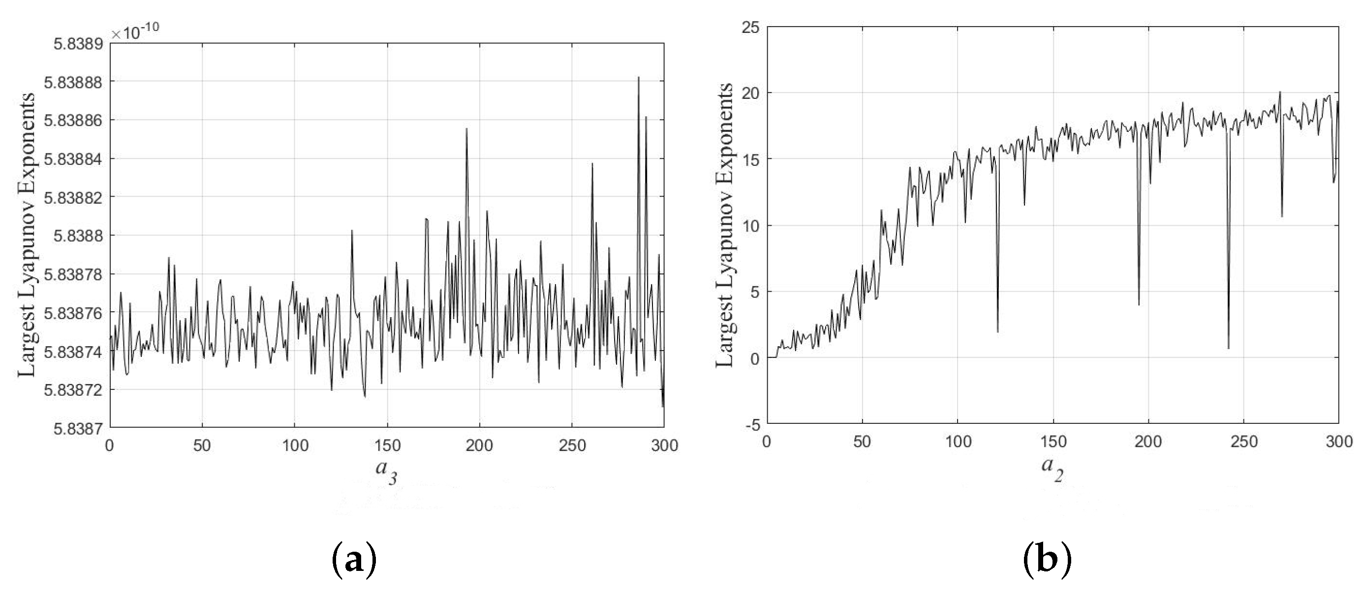
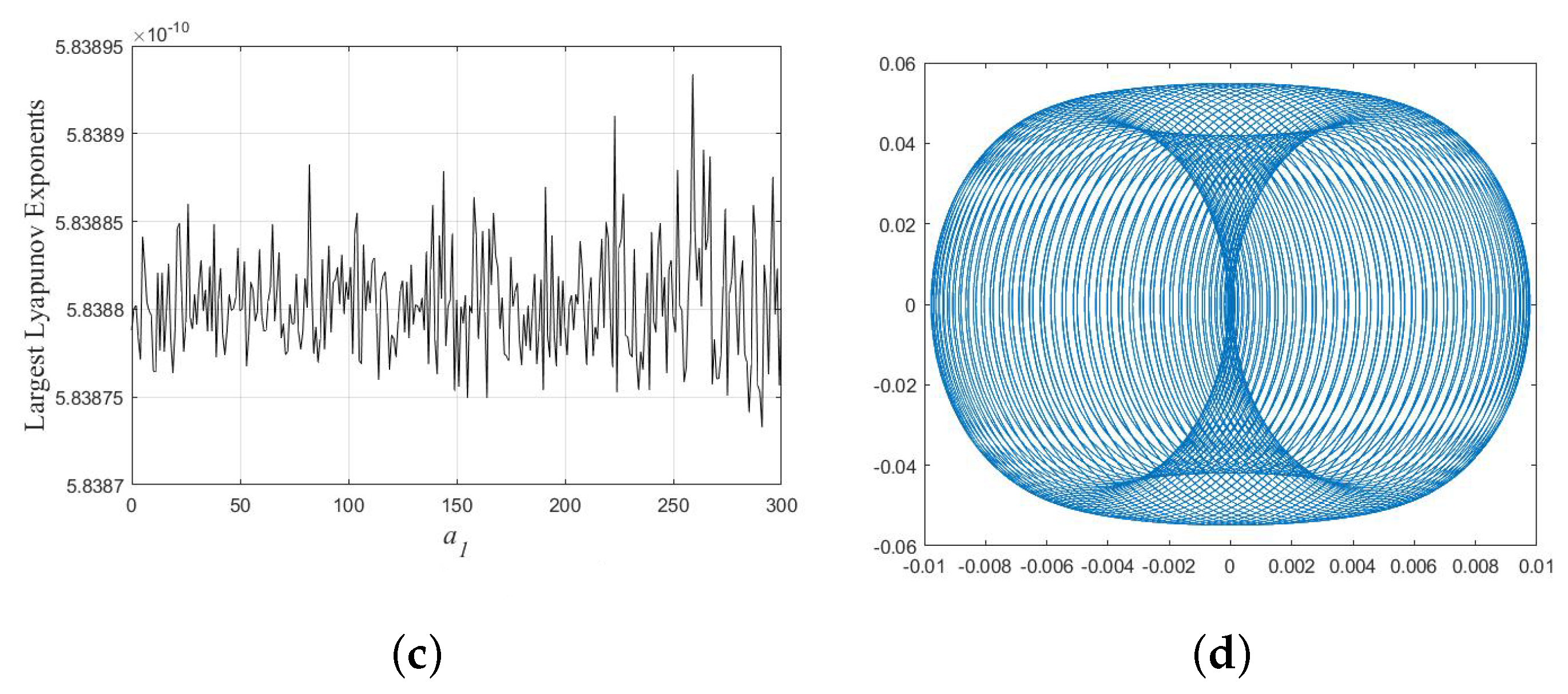
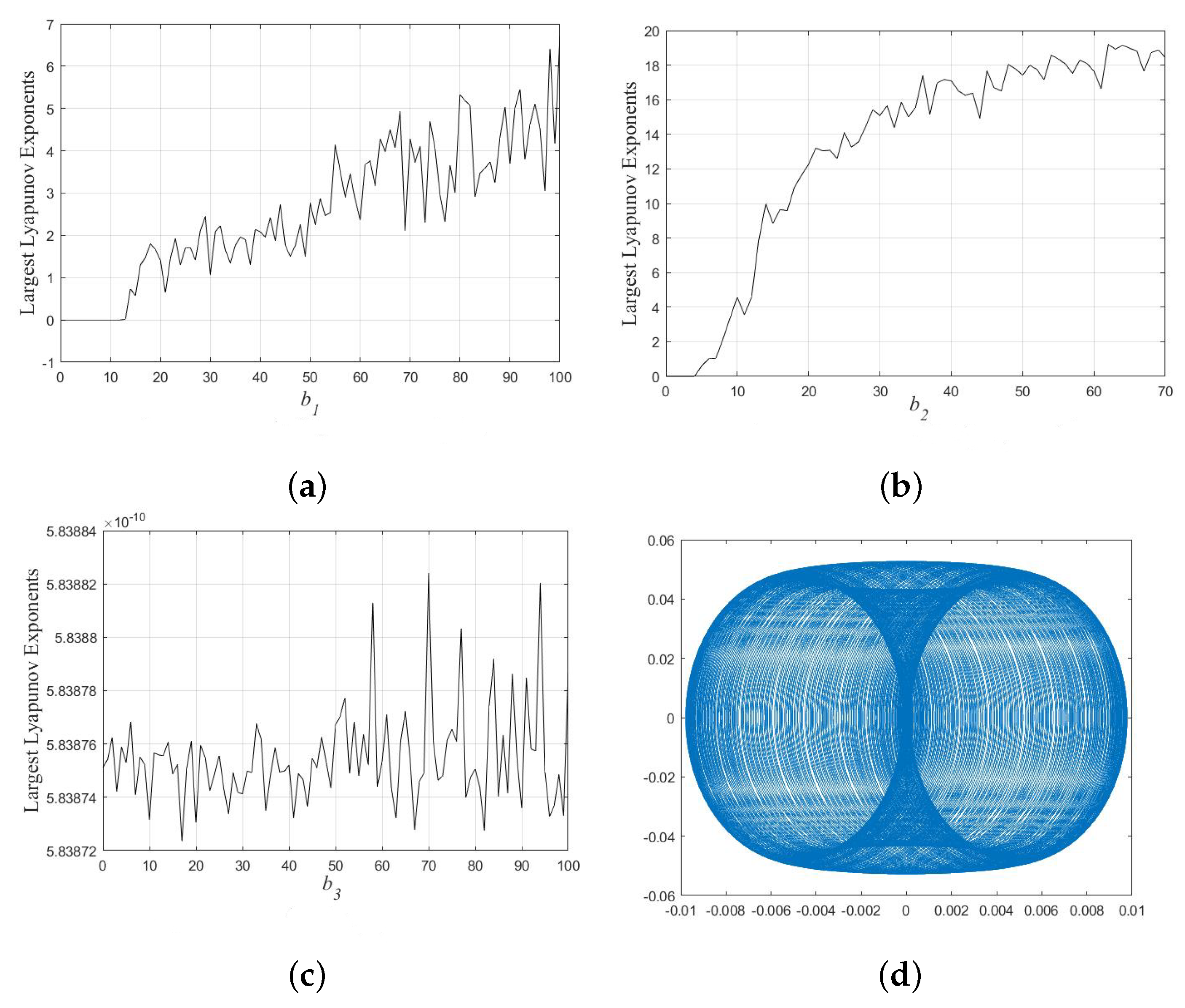
3.1. The Chaotic Motions of System (7)

We determine the nonlinear order n equal to 1 and choose three types of perturbed terms here, namely $R_i\left(\xi \right)=\sin \left(10\xi \right),\cos \left(10\xi \right)$ and $e^{0.01\xi }(i=1,2)$. Moreover, the largest Lyapunov exponents (LLE) for each situation are all shown. Concrete examples of corresponding graphs are presented in Figure 3, Figure 4 and Figure 5.

From Figure 3, Figure 4 and Figure 5, we can see that if the perturbed term is a trigonometric function, then the global phase portrait is similar to a torus. Moreover, from the three graphs, we can see that the Lyapunov exponent of $a_2$ is the largest. We could also draw the conclusion that the parameter $a_2$ is more influential than $a_3$ and $a_1$. This is also in line with our intuition since $a_2$ corresponds to the higher-order term.

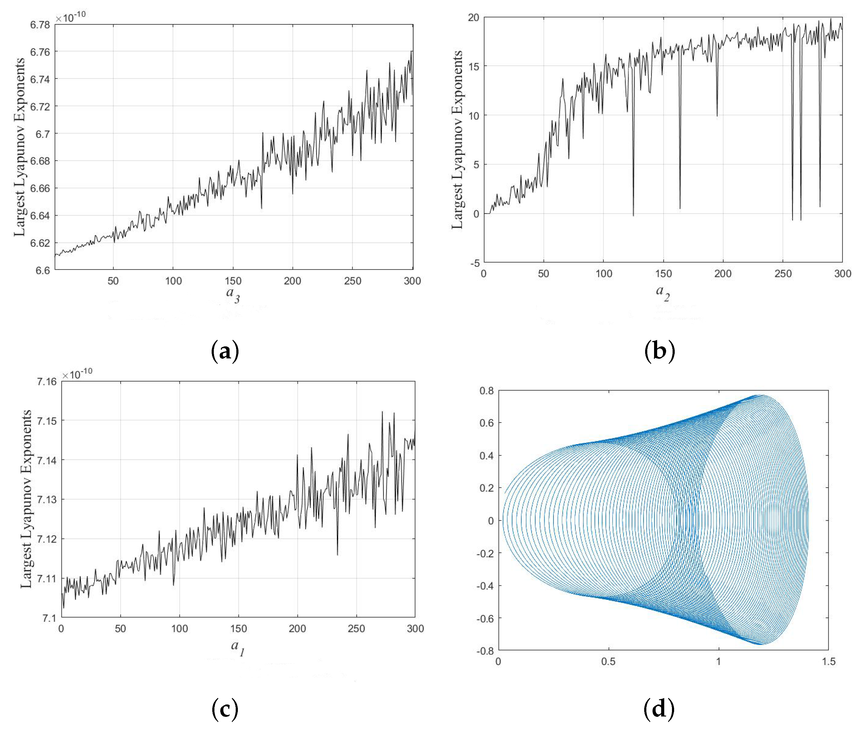
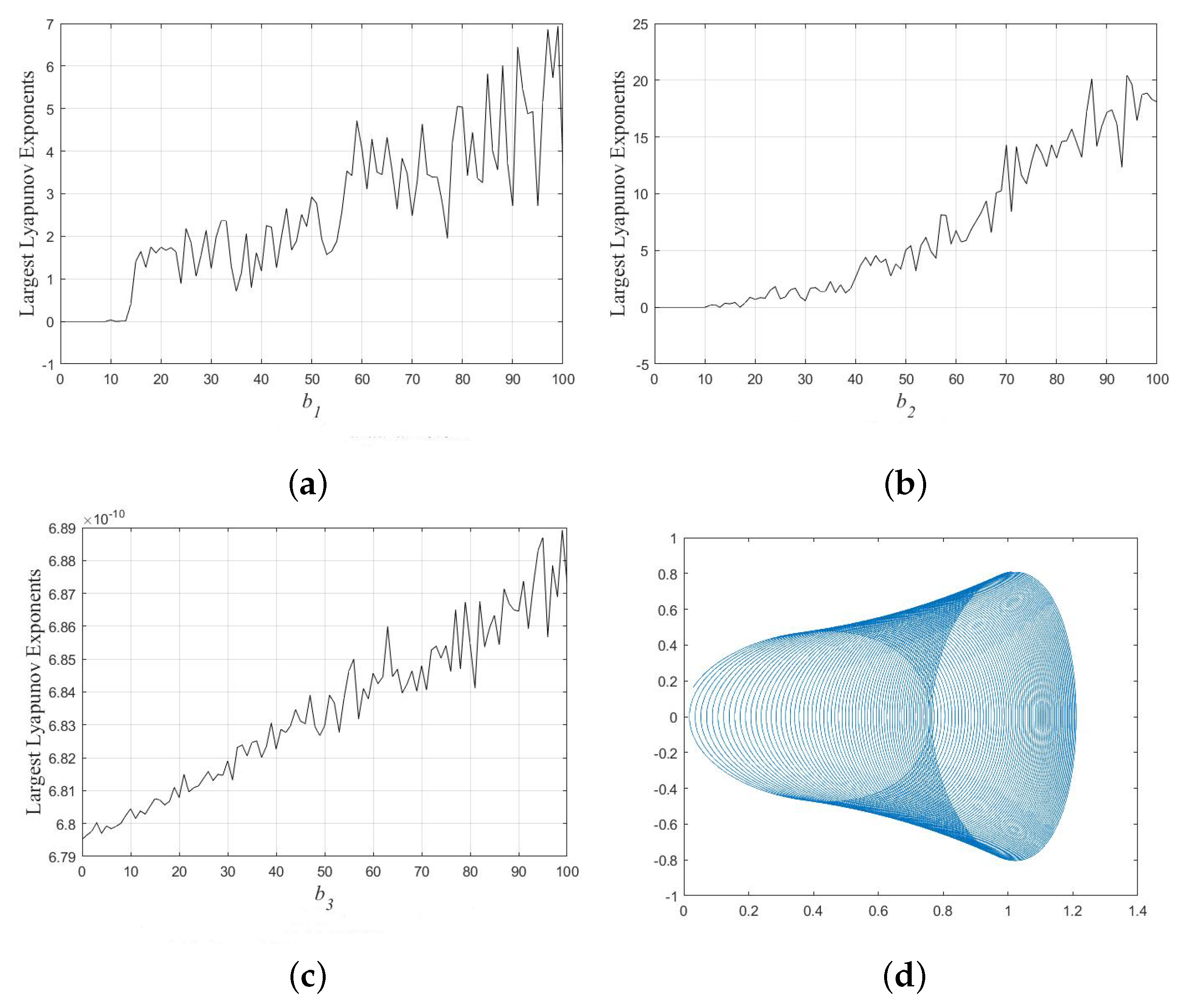
3.2. The Chaotic Motions of System (18)

We determine the nonlinear order n as 2 in system (18) and the other conditions of (18) are similar to those of system (7). The corresponding figures are given in Figure 6, Figure 7 and Figure 8.

From Figure 6, Figure 7 and Figure 8, we can see that system (18) has chaotic behaviors that are similar to system (7), so the discussion is omitted here. We also find that the parameter $b_3$ corresponds to highest-order term, but the largest Lyapunov exponent is smaller than other parameters, $b_1$ and $b_2$. This phenomenon is contrary to our common sense, thus we will leave this as an open question for future investigation.

4. Conclusions

In this paper, by taking the traveling wave transformation to ZK equation with dual-power law and triple-power law nonlinearity, we convert these equations into planner dynamic systems. Then the qualitative analysis are conducted to verify the existence of solitons and periodic solutions. From the qualitative results, we find that there are no chaotic behaviors for the non-perturbed ZK equation, so we consider adding perturbed terms to study the chaotic behaviors. According to the largest Lyapunov exponents and the corresponding phase graphs, we find that by adding the specific perturbed terms, the chaotic behaviors of the equation can be obtained. To the best of our knowledge, this is the first time that the chaotic phenomenon of the ZK equation with dual-power law and triple-power law nonlinearity is studied.

References

1. Zakharov, V.E.; Kuznetsov, E.A. Three-dimensional solitons. Zhurnal Eksperimentalnoi Teroreticheskoi Fiz. 1974, 29, 594–597. [Google Scholar]
2. Munro, S.; Parkes, E.J. The derivation of a modified Zakharov-Kuznetsov equation and the stability of its solutions. J. Plasma Phys. 2000, 62, 305–317. [Google Scholar] [CrossRef]
3. Munro, S.; Parkes, E.J. Stability of solitary-wave solutions to a modified Zakharov-Kuznetsov equation. J. Plasma Phys. 2000, 64, 411–426. [Google Scholar] [CrossRef]
4. Wazwaz, A.M. Exact solutions with solitons and periodic structures for the Zakharov-Kuznetsov (ZK) equation and its modified form. Commun. Nonlinear Sci. Numer. Simul. 2005, 10, 597–606. [Google Scholar] [CrossRef]
5. Li, B.; Yong, C.; Zhang, H. Exact travelling wave solutions for a generalized Zakharov-Kuznetsov equation. Appl. Math. Comput. 2003, 146, 653–666. [Google Scholar] [CrossRef]
6. Shivamoggi, B.K. The Painlev analysis of the Zakharov-Kuznetsov equation. Phys. Scr. 1990, 42, 641. [Google Scholar] [CrossRef]
7. Schamel, H. A modified Korteweg-de Vries equation for ion acoustic waves due to resonant electrons. J. Plasma Phys. 1973, 9, 377–387. [Google Scholar] [CrossRef]
8. Zhao, X.; Zhou, H.; Tang, Y.; Jia, H. Travelling wave solutions for modified Zakharov-Kuznetsov equation. Appl. Math. Comput. 2006, 181, 634–648. [Google Scholar] [CrossRef]
9. Biswas, A.; Zerrad, E. 1-soliton solution of the Zakharov-Kuznetsov equation with dual-power law nonlinearity. Commun. Nonlinear Sci. Numer. Simul. 2009, 14, 3574–3577. [Google Scholar] [CrossRef]
10. Du, X.X.; Tian, B.; Qu, Q.X.; Yuan, Y.Q.; Zhao, X.H. Lie group analysis, solitons, self-adjointness and conservation laws of the modified Zakharov-Kuznetsov equation in an electron-positron-ion magnetoplasma. Chaos Solitons Fractals 2020, 134, 109709. [Google Scholar] [CrossRef]
11. Jhangeer, A.; Hussain, A.; Tahir, S.; Sharif, S. Solitonic, super nonlinear, periodic, quasiperiodic, chaotic waves and conservation laws of modified Zakharov-Kuznetsov equation in transmission line. Commun. Nonlinear Sci. Numer. Simul. 2020, 86, 105254. [Google Scholar] [CrossRef]
12. Yin, H.M.; Tian, B.; Hu, C.C.; Zhao, X.C. Chaotic motions for a perturbed nonlinear Schröinger equation with the power-law nonlinearity in a nano optical fiber. Appl. Math. Lett. 2019, 93, 139–146. [Google Scholar] [CrossRef]
13. Kai, Y.; Li, Y.; Huang, L. Topological properties and wave structures of Gilson-Pickering equation. Chaos Solitons Fractals 2022, 157, 111899. [Google Scholar] [CrossRef]
14. Kai, Y.; Chen, S.; Zhang, K.; Yin, Z. Exact solutions and dynamic properties of a nonlinear fourth-order time-fractional partial differential equation. Waves Random Complex Media 2022, 1–12. [Google Scholar] [CrossRef]
Figure 1. Global phase portraits of system (12) in Case 1: (a) A = 8 ; (b) A = 8 .
Appliedmath 03 00001 g001
Figure 2. Global phase portraits of system (12) in Case 2: (a) A = 8 ; (b) A = 8 .
Appliedmath 03 00001 g002
Figure 3. System (7): (a) Largest Lyapunov Exponents for a 3 ; (b) Largest Lyapunov Exponents for a 1 ; (c) Largest Lyapunov Exponents for a 2 ; (d) Phase portrait, when a 1 = 0.9184, a 2 = 0.2232, a 3 = 1.7149, R ( ξ ) = sin ( 10 ξ ) .
Appliedmath 03 00001 g003
Figure 4. System (7): (a) Largest Lyapunov Exponents for a 3 ; (b) Largest Lyapunov Exponents for a 1 ; (c) Largest Lyapunov Exponents for a 2 ; (d) Phase portrait, when a 1 = 0.80357, a 2 = 0.4, a 3 = 1.7149, R 1 ( ξ ) = cos ( 10 ξ ) .
Appliedmath 03 00001 g004aAppliedmath 03 00001 g004b
Figure 5. System (7): (a) Largest Lyapunov Exponents for a 3 ; (b) Largest Lyapunov Exponents for a 1 ; (c) Largest Lyapunov Exponents for a 2 ; (d) Phase portrait, when a 1 = 0.80357, a 2 = 0.4, a 3 = 1.7149, R 1 ( ξ ) = e 0.01 ξ .
Appliedmath 03 00001 g005
Figure 6. System (18): (a) largest Lyapunov Exponents for b 1 ; (b) largest Lyapunov Exponents for b 2 ; (c) largest Lyapunov Exponents for b 3 ; (d) Phase portrait, when b 1 = 0.22, b 2 = 0.233, b 3 = 0.759 , b 4 = 0.178, R 2 ( ξ ) = sin ( 10 ξ ) .
Appliedmath 03 00001 g006
Figure 7. System (18): (a) largest Lyapunov Exponents for b 1 ; (b) largest Lyapunov Exponents for b 2 ; (c) largest Lyapunov Exponents for b 3 ; (d) Phase portrait, when b 1 = 0.983, b 2 = 0.33, b 3 = 0.987 , b 4 = 0.9, R 2 ( ξ ) = cos ( 10 ξ ) .
Appliedmath 03 00001 g007
Figure 8. System (18): (a) largest Lyapunov Exponents for b 1 ; (b) largest Lyapunov Exponents for b 2 ; (c) largest Lyapunov Exponents for b 3 ; (d) Phase portrait when b 1 = 0.983, b 2 = 0.33, b 3 = 0.987 , b 4 = 0.9, R 2 ( ξ ) = e 0.01 ξ .
Appliedmath 03 00001 g008
Disclaimer/Publisher’s Note: The statements, opinions and data contained in all publications are solely those of the individual author(s) and contributor(s) and not of MDPI and/or the editor(s). MDPI and/or the editor(s) disclaim responsibility for any injury to people or property resulting from any ideas, methods, instructions or products referred to in the content.