Oxygen in the Earth System

Abstract

Atmospheric oxygen is produced and consumed by life on Earth, and the ozone layer protects life on Earth from harmful solar UV radiation. The research on oxygen in the Earth system is of interest to many different geoscientific communities, from paleoclimatology to aeronomy. I provide a brief overview of the research activities and their motivations. In situ measurements and remote sensing of atmospheric oxygen are described. The global evolution, distribution, and trends of atmospheric oxygen are discussed.

1. Introduction

Molecular oxygen is the second most abundant element in the Earth’s atmosphere (21% O${}_2$ and 78% N${}_2$ by volume today). Oxygen is the most abundant element in the Earth’s crust, it accounts for 89% of the ocean mass [1]. The high abundance of atmospheric oxygen can only be explained by the continuous oxygen production from cyanobacteria, algae, and green plants. It is remarkable that the capability of oxygenic photosynthesis evolved only once on Earth. Cyanobacteria are the only creatures capable of performing this crucial process, while plants and algae rely on cyanobacterial symbionts (e.g., chloroplasts) to do this.

Oxygen chemistry, photochemistry, isotope fractionation, and ionization are crucial for the physics and chemistry of the Earth’s atmosphere. The observation of atmospheric oxygen contributes to the study of atmospheric dynamics, circulation, and energetics. Further, the global oxygen cycle is linked to the carbon cycle, which includes the dramatic increase of CO${}_2$ and, hence, global warming. Deoxygenation of the ocean is a serious problem for the health of the ocean and its aerobic life. The Earth’s ozone layer and the ionosphere have been modeled based on the assumption of a pure oxygen atmosphere [2]. Oxygen, particularly O${}^{+}$ ions, is considered a biomarker for Earth-like exoplanets. This serves as a motivation to review our knowledge of oxygen in the Earth’s system. This review article also helps to identify geoscientific research communities that are connected via the research object oxygen.

2. The Atmospheric Oxygen Cycle

The atmospheric oxygen cycle comprises all production and loss processes of atmospheric oxygen. Oxygen is mainly produced by the oxygenic photosynthesis of green plants, algae, and cyanobacteria. Oxygenic photosynthesis converts CO${}_2$ and H${}_2$O into organic matter and molecular oxygen.

$$\mathrm{C}{\mathrm{O}}_2+{\mathrm{H}}_2\mathrm{O}\leftrightarrow \mathrm{C}{\mathrm{H}}_2\mathrm{O}+{\mathrm{O}}_2$$

(1)

However, oxygen can only accumulate in the atmosphere if organic matter is buried after its lifetime without contact with the air. Otherwise, the produced oxygen would be consumed by the respiration of the organic matter after its lifetime. The abundance of atmospheric oxygen is also increased by the burial of pyrite (FeS${}_2$). Pyrite is made from seawater sulfate ions (SO${}_4^{-2}$), ferric oxide, and some organic matter, by biogeochemical processes [3]. Thus, oxygen is released. The burial of the pyrite counteracts the subsequent oxidation of the pyrite, which would reduce the oxygen abundance in the ocean and the atmosphere. A small source of oxygen is the escape of hydrogen atoms from water vapor in the upper atmosphere.

The loss of atmospheric oxygen is due to continental and submarine weathering. Volcanic activity also leads to a loss of atmospheric oxygen due to the oxidation of volcanic gases. The burning of fossil fuels and organic matter are further sinks for atmospheric oxygen.

The measurement of oxygen isotopes leads to more constraints in the description of sources and sinks in the atmospheric oxygen cycle [1]. For example, oxygen consumption by respiration of organic matter leads to a decrease of ${}^{16}$O and an accumulation of ${}^{18}$O in atmospheric oxygen (Dole effect). The oxygen isotopes are measured by mass spectrometry, interferometry, or cavity ring-down spectroscopy.

Stable isotopes in atmospheric water vapor are also considered when studying the hydrologic cycle in detail. The isotope fractionation provides information on cloud processes, precipitation, transport, and mixing [4]. For example, heavy water molecules with ${}^{18}$O condense faster and evaporate slower compared to light water molecules with ${}^{16}$O. Thus, ${}^{18}$O in atmospheric water vapor within an air parcel tends to decrease as the parcel undergoes multiple precipitation events while traveling from low to high latitudes, compared to the beginning when the water evaporates at the equator.

To measure the variability of atmospheric oxygen, it is better to measure the ratio between molecular oxygen and nitrogen. The ratio excludes fluctuations from atmospheric noise. Since the nitrogen abundance is fairly constant in the atmosphere, the ratio variations are due to changes in the oxygen concentration. The oxygen–nitrogen ratio has been measured since the 1990s in order to constrain the terrestrial and marine exchanges of CO${}_2$ [1]. The ratio and, hence, the oxygen abundance, have a negative linear trend, which is due to the increase in fossil fuel combustion. The seasonal cycle of the oxygen–nitrogen ratio is anti-correlated to the seasonal cycle of CO${}_2$ in the western North Pacific [5].

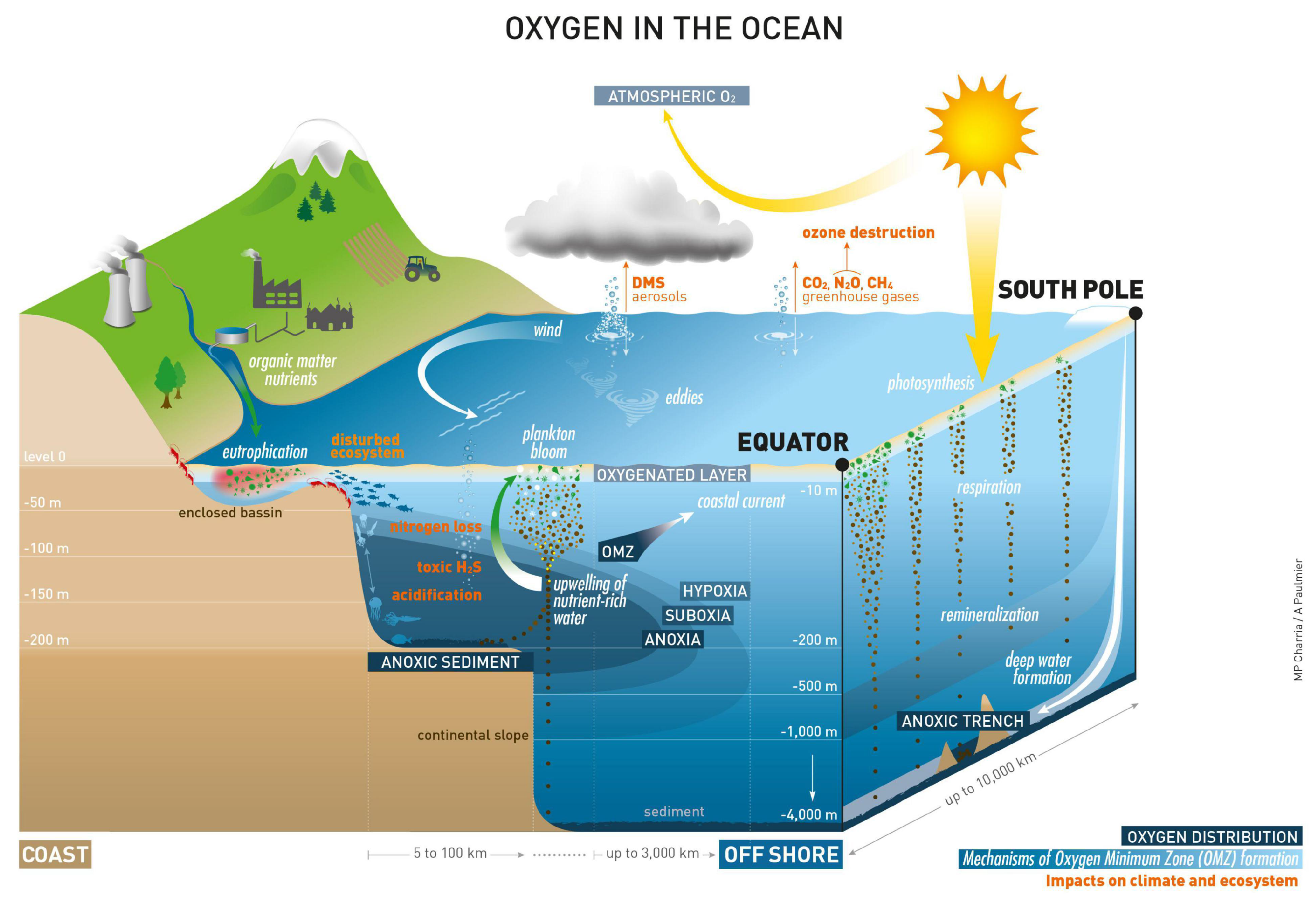
More than half of the oxygen production on the Earth comes from the ocean. On the other hand, the deoxygenation of the ocean is a serious problem for aerobic life in the ocean. Monitoring the oxygen content in the ocean by means of sensors, sondes, and platforms provides information about the health of the ocean [6]. The global ocean oxygen content decreased by about 2% (between 1960 and the 2000s), based on observations, and model projections indicate a further increase in ocean deoxygenation in the future [6]. Figure 1 shows the oxygenation and deoxygenation processes in the ocean, which are responsible for the future evolution of oxygen in the ocean.

3. The Evolution of Atmospheric Oxygen

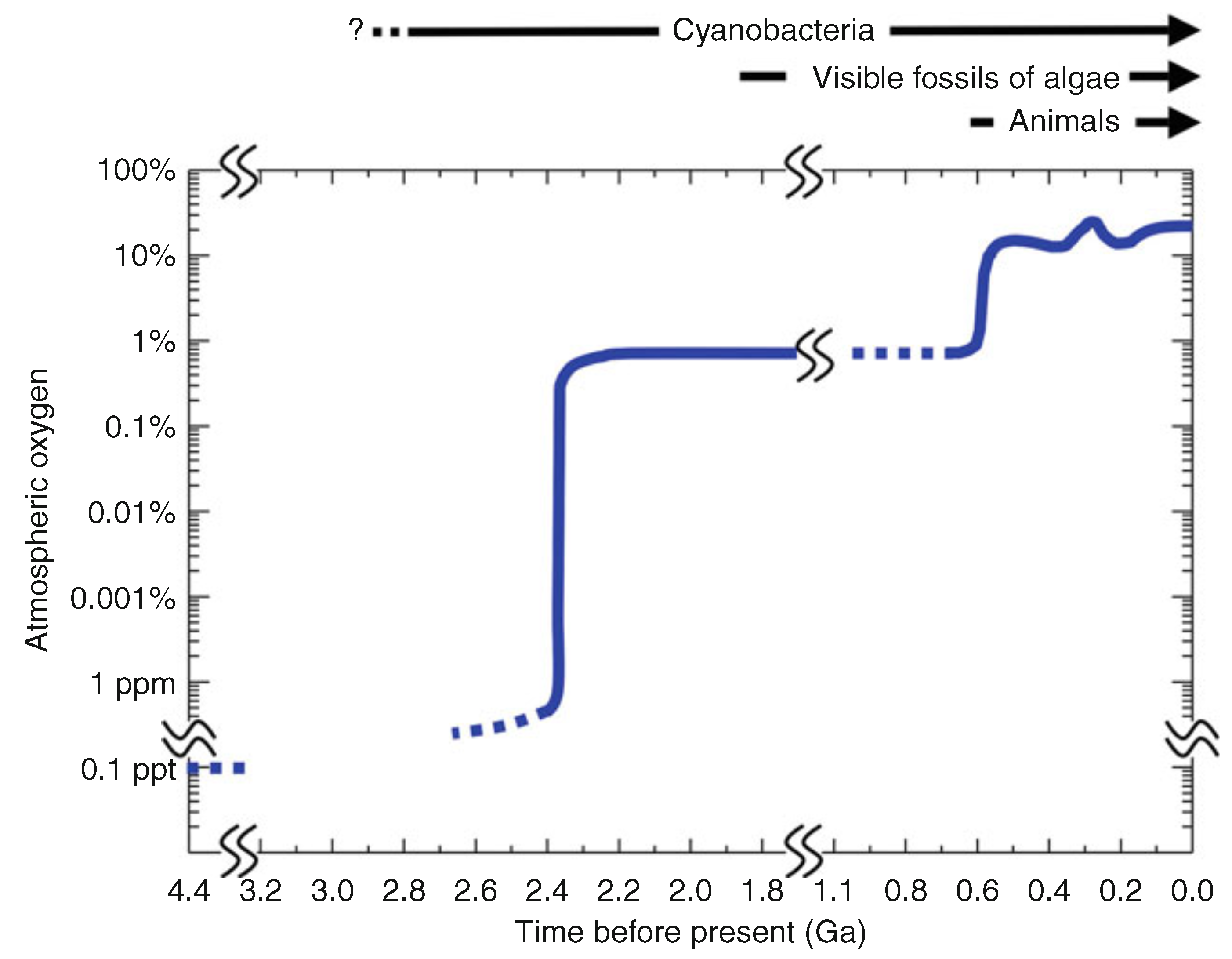
The Earth’s atmosphere turned from anoxic to oxic during the great oxidation event (GOE), which was 2.4 Gy ago. One reason was the appearance of cyanobacteria 300 My before the GOE. Additional reasons could be the decrease in the respiration of oxygen due to geologic processes, such as the appearance of continents and changes in volcanic activity [3]. During the GOE, the oxygen abundance increased from 1 ppm to 1% by volume. Figure 2 shows the evolution of atmospheric oxygen since the beginning of the Earth. The reasons for the second oxidation event at 0.6 Gy are still under investigation. After the second oxidation event, macroscopic animals appeared in the history of the Earth, and the oxygen abundance exceeded 10%. Mass spectrometry of the oxygen content in ancient rocks is required for reconstructing the past oxygen abundance.

The ${}^{18}$O isotope content in precipitation decreases with the decrease in condensation temperature [8]. Thus, oxygen isotopes in precipitation from ice-core measurements provide information about the temperature evolution from the past 100’000 years (and more). In practice, the isotopic ratio ${\delta }^{18}$O was analyzed.

$${\delta }^{18}\mathrm{O}=\frac{{{(}^{18}\mathrm{O}{/}^{16}\mathrm{O})}_{\mathrm{sample}}}{{{(}^{18}\mathrm{O}{/}^{16}\mathrm{O})}_{\mathrm{standard}}}-1$$

(2)

where the $\delta$ value is multiplied by 1000 and expressed as per mille (‰). The term Standard refers to the isotopic ratio of standard mean ocean water [1].

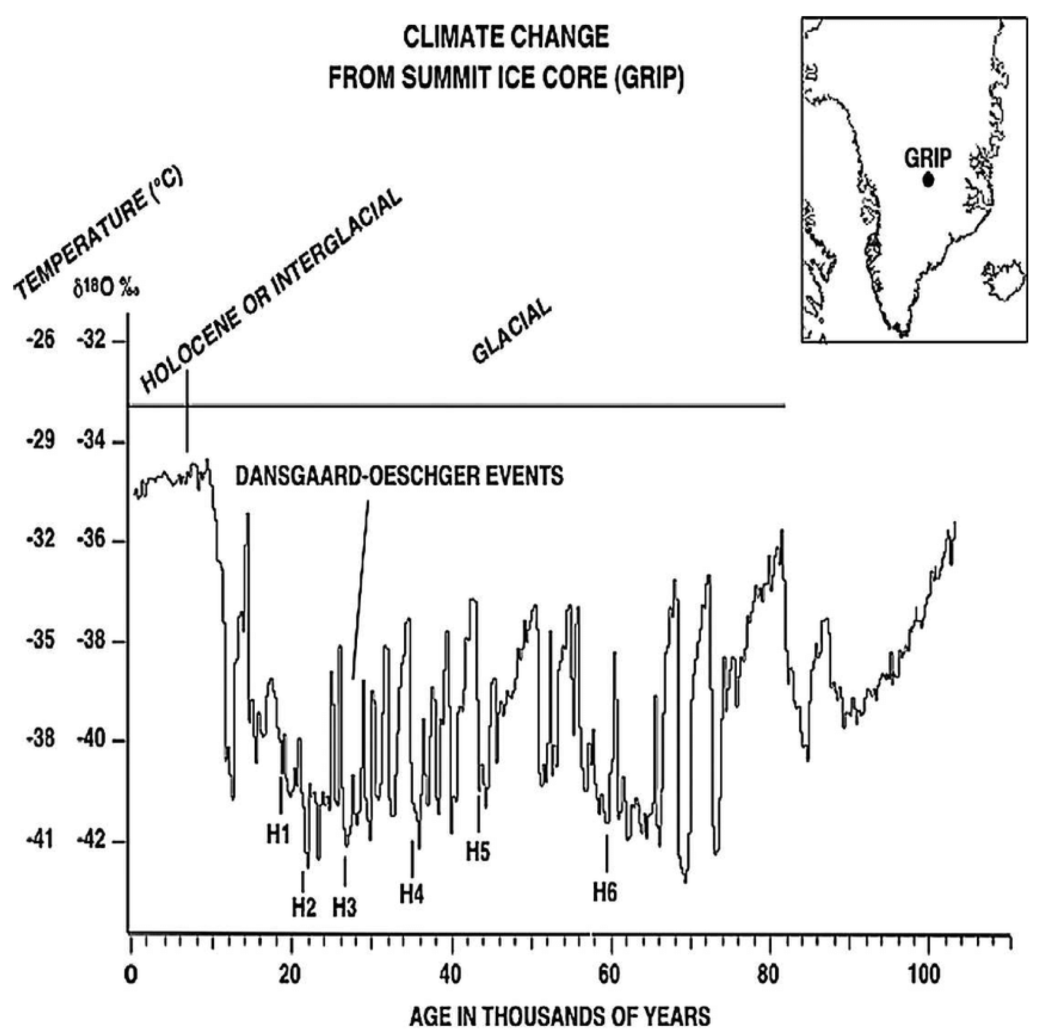
There were abrupt climate changes in the ${\delta }^{18}$O time series of the ice core from Greenland during the glacial phase (Figure 3). The rapid warming events are called Dansgaard–Oeschger events, where the temperature is between those of the glacial and interglacial phases.

4. Atmospheric Ozone

Ozone (O${}_3$) is generated by the combination of molecular and atomic oxygen. Since atomic oxygen is mainly generated by the photodissociation of molecular oxygen in the middle atmosphere, the ozone abundance is the highest in the stratosphere. The peak of the ozone concentration is at about 25 km and the ozone volume mixing ratio peaks at about 30 km in altitude in the global average, as indicated by the atmospheric ozone profile in Table A.6.2.c of [10]. The ozone molecule has a high absorption cross-section in the UV wavelength region, so the stratospheric ozone layer acts as a protection shield for life on Earth, shielding it from harmful UV radiation from the Sun. The absorption of UV radiation by ozone is responsible for the temperature increase with altitude in the stratosphere,

In the 1980s, the appearance of the ozone hole over Antarctica shocked mankind, and it was recognized that the continuous emission of man-made chlorofluorocarbons (CFCs) has to be stopped in order to save the ozone layer. In the past, the chlorine abundance increased with the increase of CFCs which are photo-dissociated at upper altitudes and later stored in HCl and ClONO${}_2$. Polar stratospheric clouds activate chlorine from the reservoir gases HCl and ClONO${}_2$, so catalytic ozone depletion by chlorine happens over Antarctica in the late winter and spring, leading to the severe depletion of the polar ozone. Without a ban on the CFC emissions, the ozone layer would have been destroyed after some decades and life on Earth would have been severely disturbed by a high UV radiance [11].

Since the 1980s, monitoring of the atmospheric ozone has been recognized as an important task in order to receive information about the state of the ozone layer, which is indispensable to life on Earth. In 2050, a recovery or even a super recovery of atmospheric ozone is expected. Ozone profiles in the troposphere and lower stratosphere (up to about 32 km high where the balloon bursts) can be obtained by ozonesondes with high vertical resolution and accuracy [12]. The sensor is an electrochemical concentration cell that measures the reaction between ozone and iodide.

4.1. Total Column Ozone

Total column ozone is the ozone column density that can be measured by Dobson and Brewer spectroradiometers on the ground. The direct solar radiation in the UV range is measured at different wavelengths. Since the absorption cross-section of ozone changes with wavelength, one obtains different intensity values. In addition, the measured intensity values also depend on the ozone column density so that the retrieval of the total column ozone is possible by using the Beer–Lambert law [13]. The solar UV intensity decreases with the increase in the total column ozone.

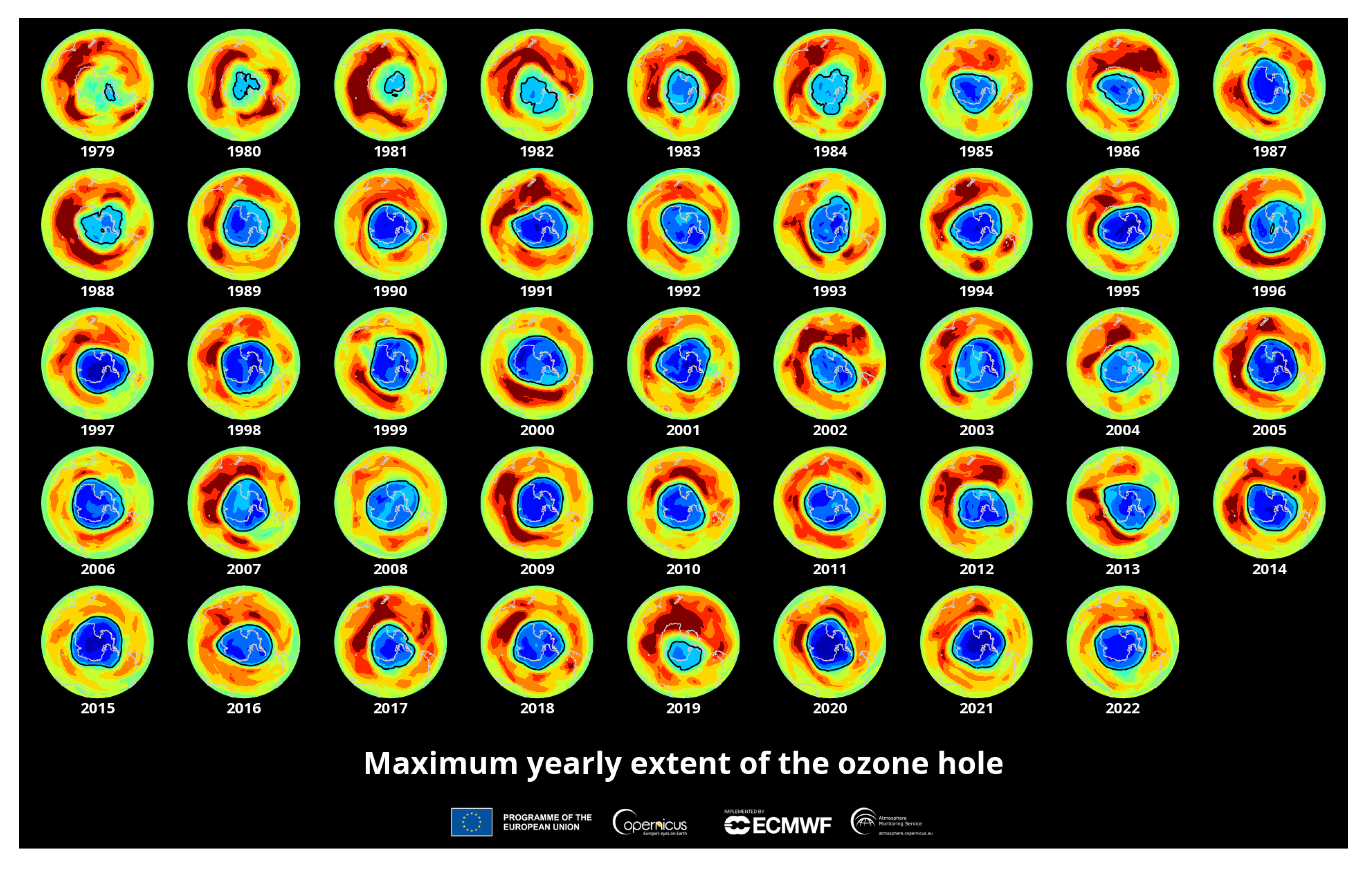
From space, the total column ozone can be observed by measuring the solar backscattered UV spectrum between 310 and 331 nm, as with the solar backscatter ultraviolet instrument (SBUV), which was flown on NOAA’s polar-orbiting operational environmental satellites (POES) [14]. Figure 4 shows the evolution of the ozone hole above Antarctica since 1979. The occurrence of the maximum yearly extent is usually around late September, corresponding to early spring in the Southern Hemisphere [15]. At this time, the polar night is over, and the sun rays photo-dissociate chlorine molecules in the polar stratosphere so that the generated chlorine atoms can start with their catalytic cycles of ozone depletion [10].

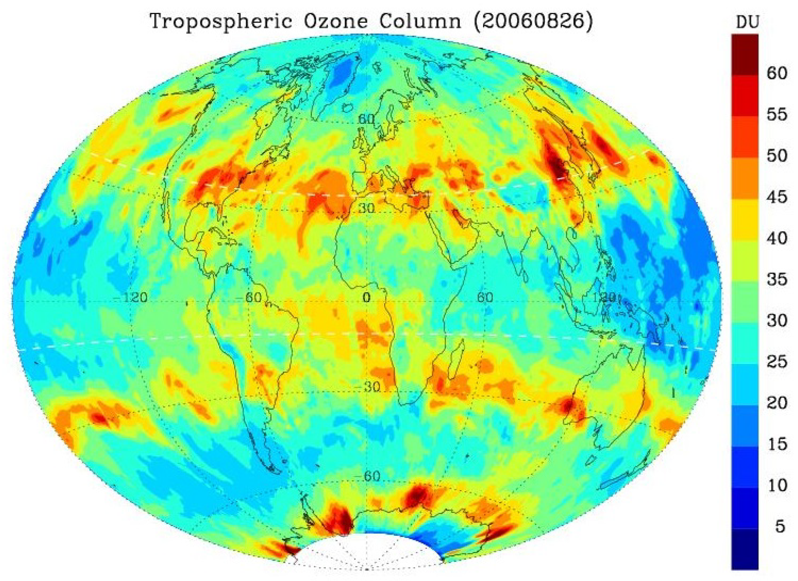
4.2. Tropospheric Ozone

About 10% of atmospheric ozone resides in the troposphere. Tropospheric ozone is mainly produced via the photodissociation of NO${}_2$, which releases atomic oxygen, which then recombines with O${}_2$ to form ozone. Volatile organic components (VOCs) reduce the amount of NO. Since NO is a sink for O${}_3$, an accumulation of tropospheric ozone is supported by a high concentration of VOCs. About 10% of tropospheric ozone is due to transport from the stratosphere [16].

Since ozone is a strong oxidant, high concentrations of ozone are harmful to the health of humans, animals, and plants. The high concentrations of NO${}_2$ and VOCs, which are due to civilization processes, such as agriculture and the combustion of fossil fuels and coal, generate, especially in the summer (a high photodissociation rate) a high concentration of tropospheric ozone, which is recognized as a serious air pollution problem. Because of the infrared absorption of ozone, tropospheric ozone is also a greenhouse gas that contributes to global warming.

Figure 4. Maximum yearly extent of the ozone hole since 1979. The ozone hole occurs in the late winter to spring. The total column ozone maps are based on satellite observations. Reproduced from [17].

Figure 4. Maximum yearly extent of the ozone hole since 1979. The ozone hole occurs in the late winter to spring. The total column ozone maps are based on satellite observations. Reproduced from [17].

The harmful effects of tropospheric ozone on life on Earth require a monitoring and warning system for tropospheric ozone as well as a reduction in anthropic emissions of NO${}_2$ and VOCs. A global map of tropospheric column ozone, obtained from the ultraviolet radiance measurements collected by the Ozone Monitoring Instrument (OMI) on the Aura satellite, is shown in Figure 5.

4.3. Stratospheric Ozone

The stratospheric ozone layer can be roughly explained by photochemical and chemical reactions in a pure oxygen atmosphere [2]. The sources and sinks of odd oxygen (atomic oxygen and ozone) are comprised of the odd oxygen cycle, which is also called the Chapman cycle:

$${\mathrm{O}}_2+h\nu \to \mathrm{O}+\mathrm{O}$$

(3)

$$\mathrm{O}+{\mathrm{O}}_2+\mathrm{M}\to {\mathrm{O}}_3+\mathrm{M}$$

(4)

$${\mathrm{O}}_3+h\nu \to \mathrm{O}+{\mathrm{O}}_2$$

(5)

$$\mathrm{O}+{\mathrm{O}}_3\to {\mathrm{O}}_2+{\mathrm{O}}_2$$

(6)

where M represents a collision partner that is inert. The atomic oxygen, which is released by ozone photodissociation, immediately recombines with molecular oxygen to form ozone again. In reality, the stratospheric ozone distribution also depends on transport processes and catalytic cycles of ozone depletion involving nitrogen, hydrogen, chlorine, and bromine species. In the polar region, heterogeneous reactions on cold polar stratospheric cloud surfaces can activate chlorine from the reservoir species ClONO₂ and HCl to form reactive species that are capable of catalytic ozone destruction in late winter to spring [19].

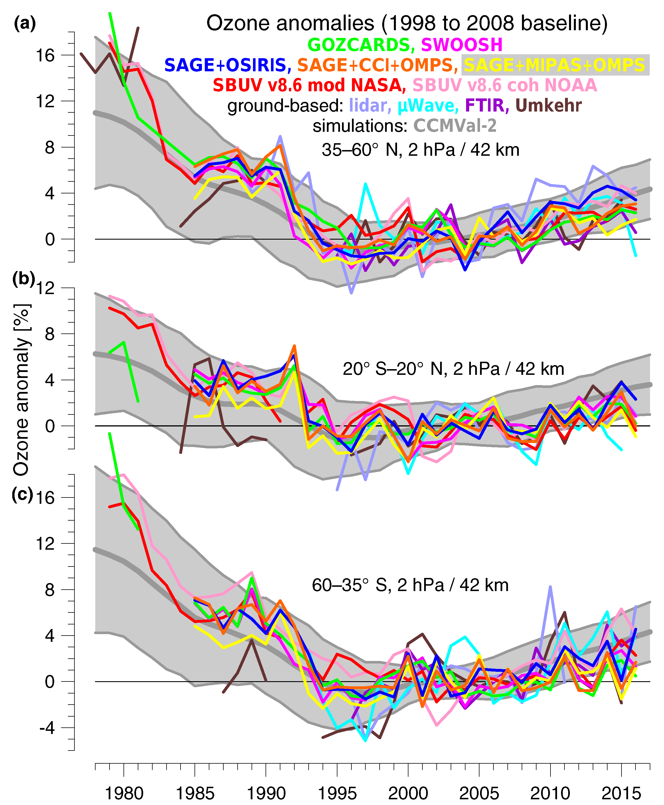
Ground-based and satellite observations and simulations by chemistry–climate models indicate positive ozone trends since 2000 in the upper stratosphere [20]. Figure 6 shows the slow increase of ozone since 2000 and the steep decrease of ozone before 1995. The slow recovery of stratospheric ozone is due to the worldwide ban on CFC emissions by the Montreal Protocol in 1987.

5. Oxygen in the Lower Atmosphere

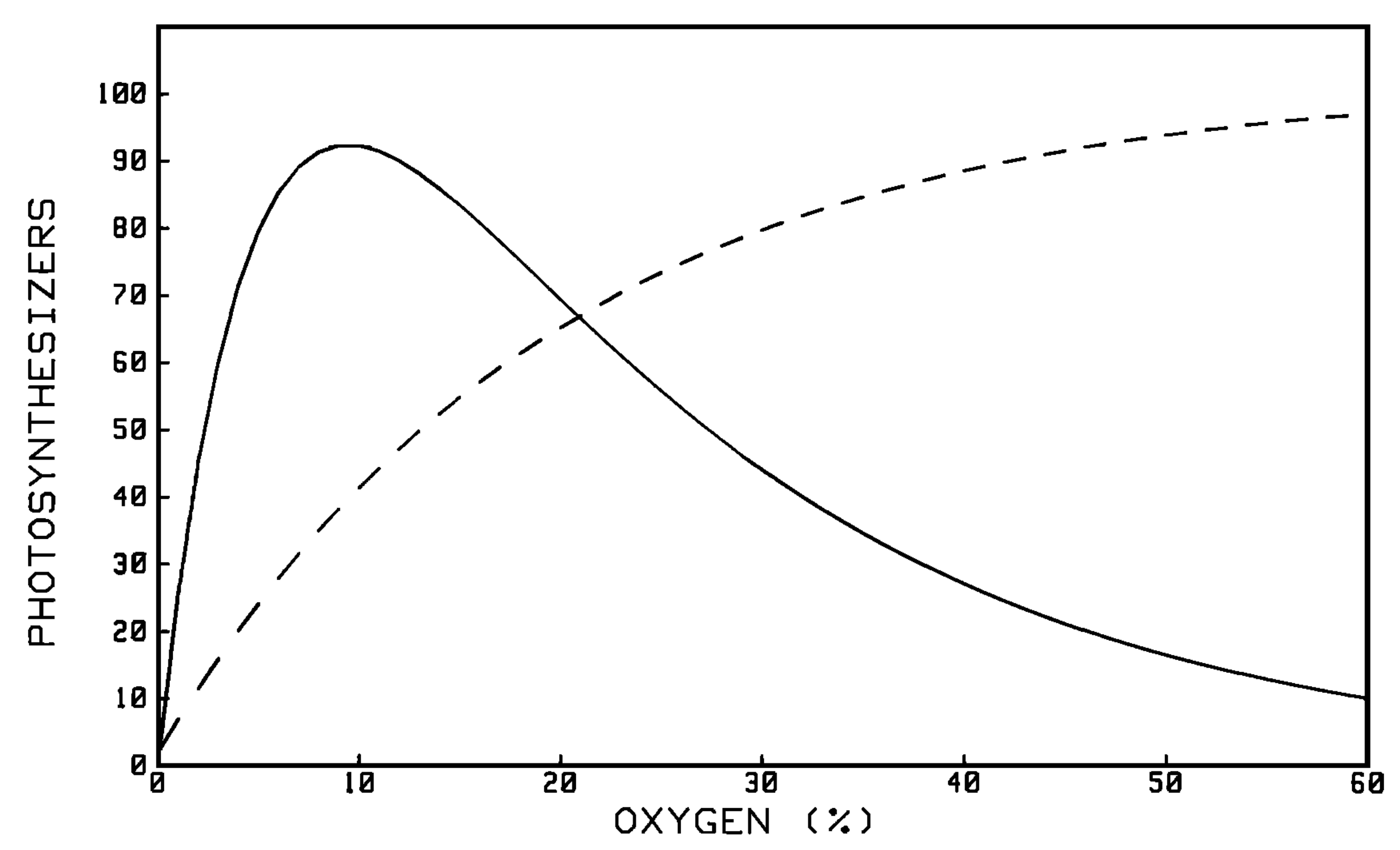
Molecular oxygen amounts to 21% by volume of the lower atmosphere. The high abundance of oxygen can only be explained by oxygenic photosynthesis carried out by life on Earth. The collision-induced fundamental vibration–rotation band at 6.4 $\mathsf{\mu }$m is the strongest absorption feature from O${}_2$ in the infrared; the Webb telescope should be able to measure the 6.4 $\mathsf{\mu }$m emission from exoplanets that have O${}_2$ abundances similar to Earth’s [21]. However, a too-high oxygen abundance is also not good and would be toxic for organisms. For example, the frequency of forest fires increases with the oxygen abundance. The oxygen abundance of the Earth has been around 21% since 0.1 Ga, and James Lovelock explained that this level is self-regulated by the Earth system. The scheme of this self-regulation is shown in Figure 7.

6. Inferring Temperature and Wind from Oxygen and Ozone Lines

Assuming a nearly constant oxygen volume mixing ratio, one can utilize the pressure-broadened oxygen emission lines in the microwave frequency range to calculate the temperature by using ground-based microwave radiometry [23]. The Doppler shift of the 142 GHz O${}_3$ line was used for the derivation of horizontal wind profiles in the stratosphere and mesosphere from observations of a ground-based microwave radiometer [24]. The temperature and geopotential height profiles from the microwave limb sounder (MLS) on the Aura satellite were derived from the observed limb radiance of the thermal oxygen emission lines at 118 and 234 GHz [25]. The Doppler shift of the 118 GHz O${}_2$ line was used for the derivation of the mesospheric wind from Aura/MLS [26]. Optical oxygen lines and bands have been utilized by various satellite missions for measuring horizontal wind profiles in the mesosphere and lower thermosphere (MLT) [27,28,29]. The wind observations of the TIMED Doppler interferometer (TIDI) on the TIMED satellite (thermosphere ionosphere mesosphere energetics and dynamics) provided valuable insight into solar tides and atmosphere dynamics in the MLT region [29].

7. Oxygen in the Middle and Upper Atmosphere

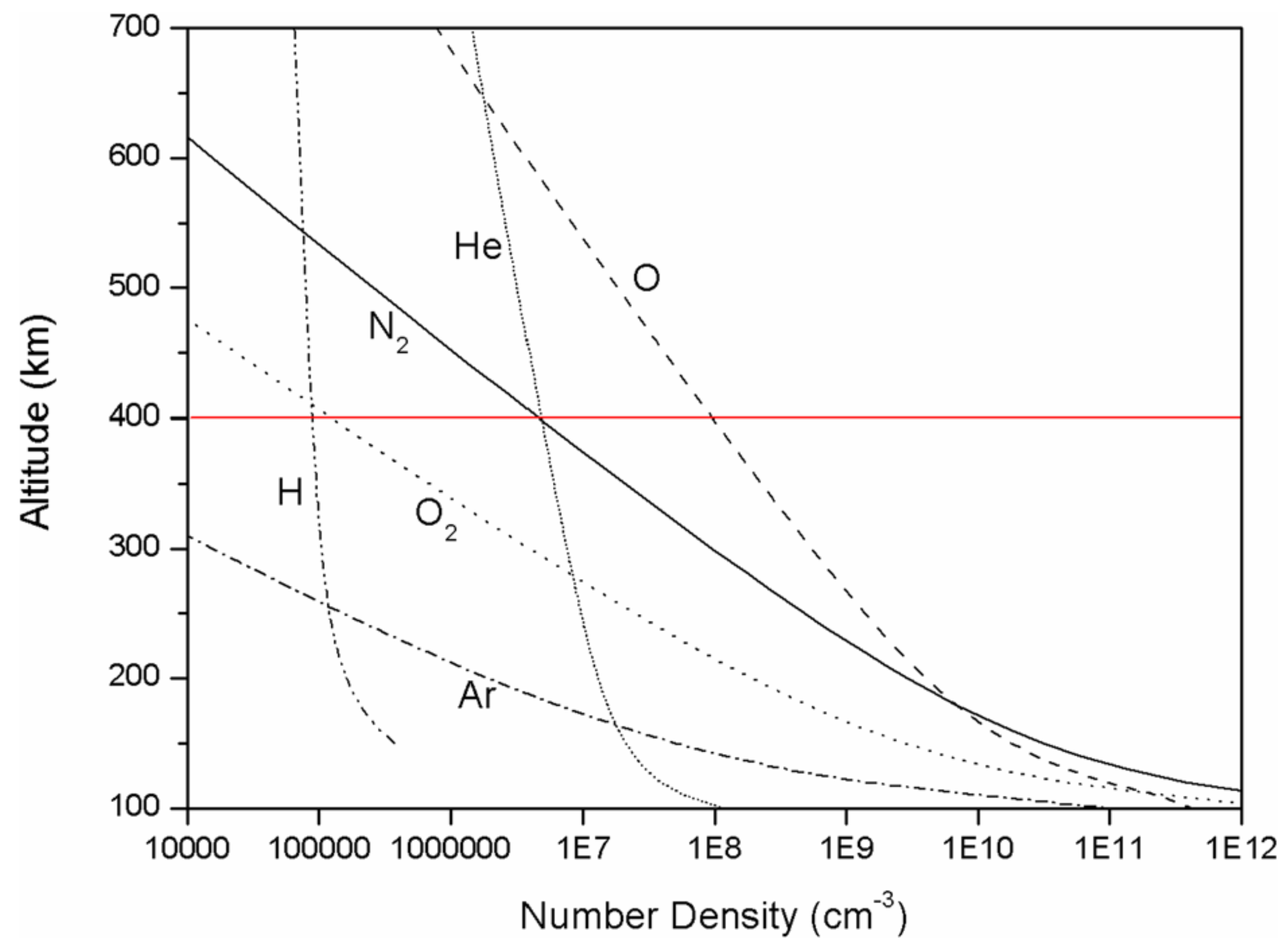
Atomic oxygen is a critical species in the chemistry and energetics of the mesosphere and lower thermosphere. The satellite instrument TIMED/SABER provided abundances of atomic oxygen and ozone [30]. Profiles of molecular oxygen and ozone can be obtained by the solar or stellar occultation technique, which considers the extinction and refraction of the starlight by oxygen and other species in the atmosphere [31,32,33]. The O${}_2$ profiles in the upper atmosphere can be measured by rockets via the absorption spectroscopy of the solar hydrogen Lyman-alpha line, which is mainly absorbed by molecular oxygen [34]. In the thermosphere, beyond 100 km high, atomic oxygen becomes the dominant species, as Figure 8 shows. Molecular oxygen is reduced in the thermosphere by photodissociation or ionization due to the intense shortwave radiation of the Sun. The red line in Figure 8 shows the typical altitude of the International Space Station (ISS). Atomic oxygen causes erosion of the material of the ISS and satellites in low Earth orbit [35].

Atomic oxygen profiles in the middle and upper atmosphere can be measured in situ by rockets with different sensors from electrolyte sensors to photometers [36]. Several optical techniques have been applied based on the emission, absorption, or fluorescence of atomic oxygen or species that are linked to it by a known reaction chain. Rocket measurements are invaluable for the refinement of reaction rates and photochemical modeling of molecular and atomic oxygen abundances [37].

Measurements of the isotopes of atomic oxygen in the mesosphere and lower thermosphere were performed for the first time via the Stratospheric Observatory for Infrared Astronomy (SOFIA) [38]. It was found that oxygen contained a higher fraction of the heavy oxygen isotope ${}^{18}$O than ocean water. The oxygen isotope fractionation of the upper atmosphere is similar to that of the lower atmosphere.

Figure 8. Composition of the thermosphere between 100 and 700 km in altitude. Data are from the U.S. Standard Atmosphere. Reproduced from [39].

Figure 8. Composition of the thermosphere between 100 and 700 km in altitude. Data are from the U.S. Standard Atmosphere. Reproduced from [39].

7.1. Gravity Waves in Airglow

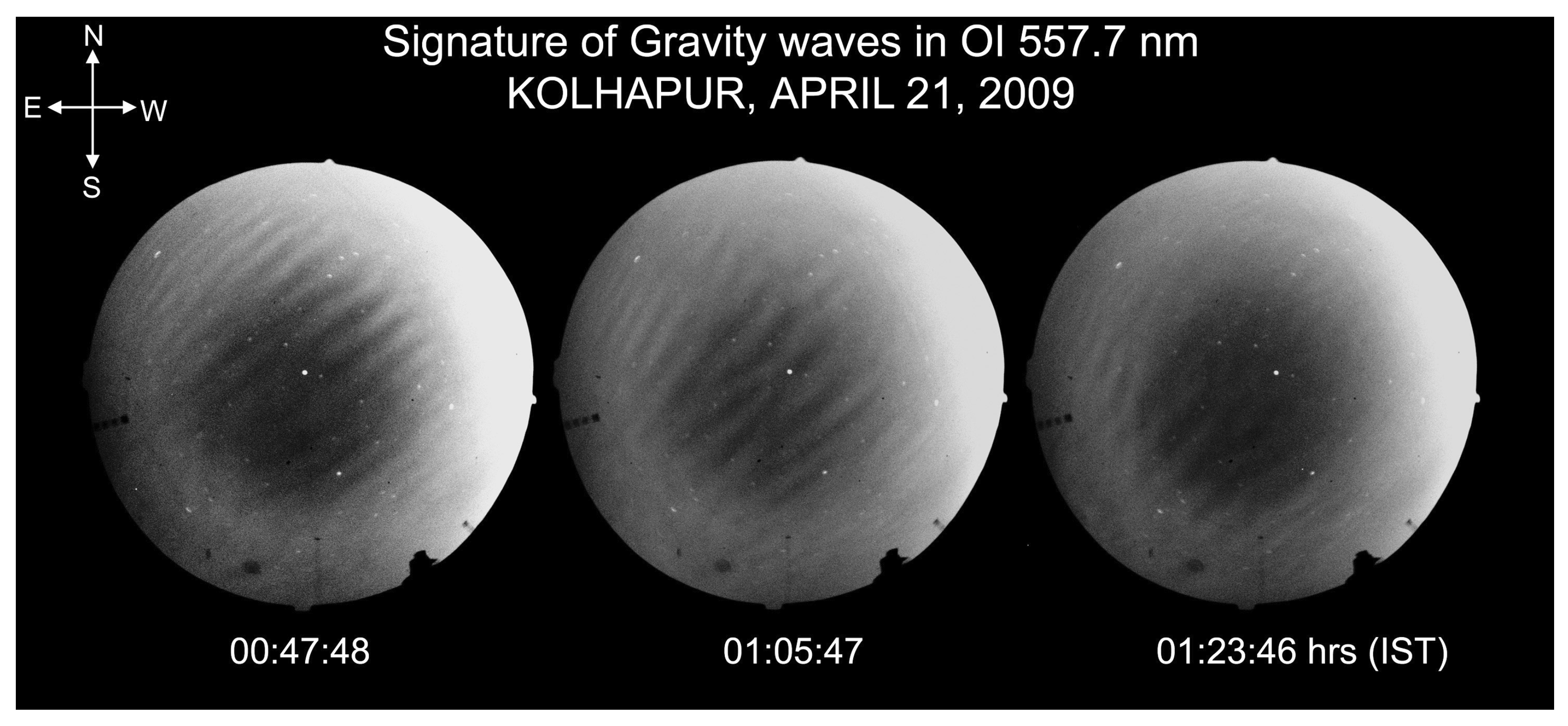
Airglow mainly occurs in the mesosphere and thermosphere, where photochemical reactions are accompanied by the emission of radiation in the visible, infrared, or ultraviolet parts of the electromagnetic spectrum [10,40,41]. Atomic oxygen has two prominent line emissions, i.e., at 557.7 nm (green light) and 630 nm (red light). Since airglow has quite a uniform distribution, it is not recognized much by the naked eye of an observer on the ground; however, contributes a significant portion of the light arriving from the sky on a moonless night [40]. Airglow is investigated to have a better understanding of the photochemistry, dynamics, and energetics of the upper atmosphere. Atmospheric waves induce spatial–temporal variations in the airglow. All sky airglow imagers on the ground can be used to observe mesospheric gravity waves. The movements of the wave ripples provide information about the wave propagation speed, wave period, horizontal wavelength, and other wave parameters. The signatures of mesospheric gravity waves are depicted in Figure 9. The knowledge of gravity waves is crucial since momentum and energy deposits by gravity waves determine the circulation of the middle and upper atmosphere.

Airglow observations are also performed by satellites and the International Space Station [43]. From space, the airglow in the O${}_2$ band is a good option since the surface light noise is reduced due to the absorption by lower atmospheric O${}_2$.

7.2. Aurora

Different from airglow, the aurora is energized by charged particles from the solar wind and the Earth’s magnetosphere. Collisions of the particles with atmospheric molecules or atoms can induce excited states and subsequent line emissions. The green oxygen aurora and the green airglow are both caused by the same line transition at 557.7 nm, and the red aurora is at 630 nm, which is also known to be present in airglow. Aurora is also interesting for research on exoplanets. A green aurora indicates that a planet has oxygen. Radio wave emissions are associated with aurora and such exoplanet emissions are already detectable by radio telescopes [44]. The auroral radio waves indicate that there is an exoplanet and that the exoplanet is protected by a magnetosphere.

7.3. Oxygen Ions in the Ionosphere and Magnetosphere

Atomic oxygen is the dominant species in the F${}_2$ region of the ionosphere, where the peak electron density is about 300 to 400 km high. Atomic oxygen ions O${}^{+}$ are the dominant ion species in the ionospheric F${}_2$ region. Oxygen ions also occur on other planets; Mars and Venus have maxima for O${}_2^{+}$. Mendillo et al. proposed that the dominance of O${}^{+}$ ions in the ionospheric composition at the altitude of maximum electron density can be used to identify a planet in orbit around a solar-type star where global-scale biological activity is present [45]. In the optical domain (ultraviolet, visible, and infrared), O${}^{+}$ ions can be detected directly via resonantly scattered starlight, by the photons emitted by the recombination of O${}^{+}$ ions and electrons, and by absorption-line spectroscopy [45].

The discovery of high concentrations of O${}^{+}$ ions in the Earth’s magnetosphere was a great surprise in 1972, when a satellite in a polar orbit around the Earth, operating in a low Earth orbit, measured significant heavy ion fluxes during the main phase of a geomagnetic storm [46,47]. The mass spectrometer on the satellite detected a peak corresponding to the M/q ratio 16. Previously, it was assumed that the energies of oxygen ions are too small for an escape from the ionosphere and for a transfer from the ionosphere into the magnetosphere. Thus, it was believed that the magnetospheric ion composition would be dominated by the light ions of hydrogen and helium from the solar wind. However, it was observed that during geomagnetic storms, oxygen ions are the dominant species in the ring current and magnetotail of the Earth’s magnetosphere. The ionospheric outflow occurs at high latitudes, where the oxygen ions have energies between 0.7 and 12 keV/e due to electrodynamical processes in the polar ionosphere. These energies are sufficient to escape Earth’s gravity and to populate the magnetosphere [47].

8. Conclusions

Considering all the important studies in the different fields of oxygen research in geosciences seems to be impossible and would result in a very long and unreadable article. However, it was worth it to provide a brief overview of the geoscientific areas in order to obtain an impression about oxygen in the Earth system. Such an overview is interesting for many different geoscientific research communities and is a gateway to related studies on oxygen. The initial scope of this article was focused on “atmospheric oxygen”; however, during the study, I noticed that the oxygen cycle and the role of oxygen in the ocean are important areas that should also be considered. Moreover, oxygen ions in the ionosphere and magnetosphere are of interest, as well as research on the possible detection of oxygen on habitable exoplanets.

References

- Keeling, R.F. The atmospheric oxygen cycle: The oxygen isotopes of atmospheric CO2 and 02 and the 02/N2 ratio. Rev. Geophys. 1995, 33, 1253–1262. [Google Scholar] [CrossRef]
- Chapman, S. The absorption and dissociative or ionizing effect of monochromatic radiation in an atmosphere on a rotating earth. Proc. Phys. Soc. 1931, 43, 26–45. [Google Scholar] [CrossRef]
- Catling, D.C. Oxygenation of the Earth’s Atmosphere. In Encyclopedia of Astrobiology; Gargaud, M., Irvine, W.M., Amils, R., Cleaves, H.J.J., Pinti, D.L., Quintanilla, J.C., Rouan, D., Spohn, T., Tirard, S., Viso, M., Eds.; Springer: Berlin/Heidelberg, Germany, 2015; pp. 1816–1826. [Google Scholar] [CrossRef]
- Galewsky, J.; Steen-Larsen, H.C.; Field, R.D.; Worden, J.; Risi, C.; Schneider, M. Stable isotopes in atmospheric water vapor and applications to the hydrologic cycle. Rev. Geophys. 2016, 54, 809–865. [Google Scholar] [CrossRef]
- Ishidoya, S.; Tsuboi, K.; Niwa, Y.; Matsueda, H.; Murayama, S.; Ishijima, K.; Saito, K. Spatiotemporal variations of the δ(O2 / N2), CO2 and δ(APO) in the troposphere over the western North Pacific. Atmos. Chem. Phys. 2022, 22, 6953–6970. [Google Scholar] [CrossRef]
- Grégoire, M.; Garçon, V.; Garcia, H.; Breitburg, D.; Isensee, K.; Oschlies, A.; Telszewski, M.; Barth, A.; Bittig, H.C.; Carstensen, J.; et al. A Global Ocean Oxygen Database and Atlas for Assessing and Predicting Deoxygenation and Ocean Health in the Open and Coastal Ocean. Front. Mar. Sci. 2021, 8. [Google Scholar] [CrossRef]
- Paulmier, A. Oxygen and the ocean. In The Ocean Revealed; Euzen, A., Gaill, F., Lacroix, D., Cury, P., Eds.; CNRS: Paris, France, 2017; pp. 48–49. [Google Scholar]
- Dansgaard, W. Stable isotopes in precipitation. Tellus 1964, 16, 436–468. [Google Scholar] [CrossRef]
- Cane, M.A.; Braconnot, P.; Clement, A.; Gildor, H.; Joussaume, S.; Kageyama, M.; Khodri, M.; Paillard, D.; Tett, S.; Zorita, E. Progress in Paleoclimate Modeling. J. Clim. 2006, 19, 5031–5057. [Google Scholar] [CrossRef] [Green Version]
- Brasseur, G.P.; Solomon, S. Aeronomy of the Middle Atmosphere: Chemistry and Physics of the Stratosphere and Mesosphere, 3rd ed.; Springer: Dordrecht, The Netherland, 2005; p. 644. [Google Scholar]
- Newman, P.A.; Oman, L.D.; Douglass, A.R.; Fleming, E.L.; Frith, S.M.; Hurwitz, M.M.; Kawa, S.R.; Jackman, C.H.; Krotkov, N.A.; Nash, E.R.; et al. What would have happened to the ozone layer if chlorofluorocarbons (CFCs) had not been regulated? Atmos. Chem. Phys. 2009, 9, 2113–2128. [Google Scholar] [CrossRef] [Green Version]
- Tarasick, D.W.; Smit, H.G.J.; Thompson, A.M.; Morris, G.A.; Witte, J.C.; Davies, J.; Nakano, T.; Van Malderen, R.; Stauffer, R.M.; Johnson, B.J.; et al. Improving ECC Ozonesonde Data Quality: Assessment of Current Methods and Outstanding Issues. Earth Space Sci. 2021, 8, e2019EA000914. [Google Scholar] [CrossRef]
- Gröbner, J.; Schill, H.; Egli, L.; Stübi, R. Consistency of total column ozone measurements between the Brewer and Dobson spectroradiometers of the LKO Arosa and PMOD/WRC Davos. Atmos. Meas. Tech. 2021, 14, 3319–3331. [Google Scholar] [CrossRef]
- Bhartia, P.K.; McPeters, R.D.; Flynn, L.E.; Taylor, S.; Kramarova, N.A.; Frith, S.; Fisher, B.; DeLand, M. Solar Backscatter UV (SBUV) total ozone and profile algorithm. Atmos. Meas. Tech. 2013, 6, 2533–2548. [Google Scholar] [CrossRef] [Green Version]
- World Meteorological Organization. The Ozone Hole. 2023. Available online: https://www.theozonehole.org/wmoozone.htm (accessed on 16 June 2023).
- Yu, R.; Lin, Y.; Zou, J.; Dan, Y.; Cheng, C. Review on Atmospheric Ozone Pollution in China: Formation, Spatiotemporal Distribution, Precursors and Affecting Factors. Atmosphere 2021, 12, 1675. [Google Scholar] [CrossRef]
- Copernicus Atmosphere Monitoring Service. Three Peculiar Antarctic Ozone Hole Seasons. 2023. Available online: https://atmosphere.copernicus.eu/three-peculiar-antarctic-ozone-hole-seasons-row-what-we-know (accessed on 16 June 2023).
- Liu, X.; Bhartia, P.K.; Chance, K.; Spurr, R.J.D.; Kurosu, T.P. Ozone profile retrievals from the Ozone Monitoring Instrument. Atmos. Chem. Phys. 2010, 10, 2521–2537. [Google Scholar] [CrossRef] [Green Version]
- Solomon, S.; Garcia, R.R.; Rowland, F.S.; Wuebbles, D.J. On the depletion of Antarctic ozone. Nature 1986, 321, 755–758. [Google Scholar] [CrossRef] [Green Version]
- Steinbrecht, W.; Froidevaux, L.; Fuller, R.; Wang, R.; Anderson, J.; Roth, C.; Bourassa, A.; Degenstein, D.; Damadeo, R.; Zawodny, J.; et al. An update on ozone profile trends for the period 2000 to 2016. Atmos. Chem. Phys. 2017, 17, 10675–10690. [Google Scholar] [CrossRef] [Green Version]
- Fauchez, T.J.; Villanueva, G.L.; Schwieterman, E.W.; Turbet, M.; Arney, G.; Pidhorodetska, D.; Kopparapu, R.K.; Mandell, A.; Domagal-Goldman, S.D. Sensitive probing of exoplanetary oxygen via mid-infrared collisional absorption. Nat. Astron. 2020, 4, 372–376. [Google Scholar] [CrossRef] [Green Version]
- Lovelock, J.E. Geophysiology, the science of Gaia. Rev. Geophys. 1989, 27, 215–222. [Google Scholar] [CrossRef]
- Krochin, W.; Stober, G.; Murk, A. Development of a Polarimetric 50-GHz Spectrometer for Temperature Sounding in the Middle Atmosphere. IEEE J. Sel. Top. Appl. Earth Obs. Remote Sens. 2022, 15, 5644–5651. [Google Scholar] [CrossRef]
- Rüfenacht, R.; Murk, A.; Kämpfer, N.; Eriksson, P.; Buehler, S.A. Middle-atmospheric zonal and meridional wind profiles from polar, tropical and midlatitudes with the ground-based microwave Doppler wind radiometer WIRA. Atmos. Meas. Tech. 2014, 7, 4491–4505. [Google Scholar] [CrossRef] [Green Version]
- Schwartz, M.J.; Lambert, A.; Manney, G.L.; Read, W.G.; Livesey, N.J.; Froidevaux, L.; Ao, C.O.; Bernath, P.F.; Boone, C.D.; Cofield, R.E.; et al. Validation of the Aura Microwave Limb Sounder temperature and geopotential height measurements. J. Geophys. Res. Atmos. 2008, 113. [Google Scholar] [CrossRef] [Green Version]
- Wu, D.L.; Schwartz, M.J.; Waters, J.W.; Limpasuvan, V.; Wu, Q.; Killeen, T.L. Mesospheric doppler wind measurements from Aura Microwave Limb Sounder (MLS). Adv. Space Res. 2008, 42, 1246–1252. [Google Scholar] [CrossRef]
- Fleming, E.L.; Chandra, S.; Burrage, M.D.; Skinner, W.R.; Hays, P.B.; Solheim, B.H.; Shepherd, G.G. Climatological mean wind observations from the UARS high-resolution Doppler imager and wind imaging interferometer: Comparison with current reference models. J. Geophys. Res. Atmos. 1996, 101, 10455–10473. [Google Scholar] [CrossRef]
- McLandress, C.; Shepherd, G.G.; Solheim, B.H. Satellite observations of thermospheric tides: Results from the Wind Imaging Interferometer on UARS. J. Geophys. Res. Atmos. 1996, 101, 4093–4114. [Google Scholar] [CrossRef]
- Killeen, T.L.; Wu, Q.; Solomon, S.C.; Ortland, D.A.; Skinner, W.R.; Niciejewski, R.J.; Gell, D.A. TIMED Doppler Interferometer: Overview and recent results. J. Geophys. Res. Space Phys. 2006, 111, A10S01. [Google Scholar] [CrossRef]
- Mlynczak, M.G.; Hunt, L.A.; Russell, J.M., III; Marshall, B.T. Updated SABER Night Atomic Oxygen and Implications for SABER Ozone and Atomic Hydrogen. Geophys. Res. Lett. 2018, 45, 5735–5741. [Google Scholar] [CrossRef]
- Hays, P.; Roble, R. Stellar occultation measurements of molecular oxygen in the lower thermosphere. Planet. Space Sci. 1973, 21, 339–348. [Google Scholar] [CrossRef] [Green Version]
- Yee, J.H.; Vervack, R.J., Jr.; DeMajistre, R.; Morgan, F.; Carbary, J.F.; Romick, G.J.; Morrison, D.; Lloyd, S.A.; DeCola, P.L.; Paxton, L.J.; et al. Atmospheric remote sensing using a combined extinctive and refractive stellar occultation technique 1. Overview and proof-of-concept observations. J. Geophys. Res. Atmos. 2002, 107, ACH 15-1–ACH 15-13. [Google Scholar] [CrossRef]
- Sun, M.; Dong, X.; Zhu, Q.; Cheng, X.; Wang, H.; Wu, J. Comparison and Analysis of Stellar Occultation Simulation Results and SABER-Satellite-Measured Data in Near Space. Remote Sens. 2022, 14, 5065. [Google Scholar] [CrossRef]
- Quessette, J.A. On the measurement of molecular oxygen concentration by absorption spectroscopy. J. Geophys. Res. 1970, 75, 839–844. [Google Scholar] [CrossRef]
- Osborne, J.J.; Harris, I.L.; Roberts, G.T.; Chambers, A.R. Satellite and rocket-borne atomic oxygen sensor techniques. Rev. Sci. Instrum. 2001, 72, 4025–4041. [Google Scholar] [CrossRef]
- Eberhart, M.; Löhle, S.; Steinbeck, A.; Binder, T.; Fasoulas, S. Measurement of atomic oxygen in the middle atmosphere using solid electrolyte sensors and catalytic probes. Atmos. Meas. Tech. 2015, 8, 3701–3714. [Google Scholar] [CrossRef] [Green Version]
- Lednyts’kyy, O.; von Savigny, C. Photochemical modeling of molecular and atomic oxygen based on multiple nightglow emissions measured in situ during the Energy Transfer in the Oxygen Nightglow rocket campaign. Atmos. Chem. Phys. 2020, 20, 2221–2261. [Google Scholar] [CrossRef] [Green Version]
- Wiesemeyer, H.; Güsten, R.; Aladro, R.; Klein, B.; Hübers, H.W.; Richter, H.; Graf, U.U.; Justen, M.; Okada, Y.; Stutzki, J. First detection of the atomic 18O isotope in the mesosphere and lower thermosphere of Earth. Phys. Rev. Res. 2023, 5, 013072. [Google Scholar] [CrossRef]
- Cottin, H.; Kotler, J.M.; Billi, D.; Cockell, C.; Demets, R.; Ehrenfreund, P.; Elsaesser, A.; d’Hendecourt, L.; van Loon, J.J.W.A.; Martins, Z.; et al. Space as a Tool for Astrobiology: Review and Recommendations for Experimentations in Earth Orbit and Beyond. Space Sci. Rev. 2017, 209, 83–181. [Google Scholar] [CrossRef] [Green Version]
- Hargreaves, J.K. The Solar-Terrestrial Environment: An Introduction to Geospace—The Science of the Terrestrial Upper Atmosphere, Ionosphere, and Magnetosphere; Cambridge Atmospheric and Space Science Series; Cambridge University Press: Cambridge, UK, 1992. [Google Scholar] [CrossRef]
- Rees, M.H. Physics and Chemistry of the Upper Atmosphere; Cambridge University Press: Cambridge, UK, 1989. [Google Scholar]
- Mukherjee, G.; Sikha, P.; Parihar, N.; Ghodpage, R.; Tukaram, P. Studies of the wind filtering effect of gravity waves observed at Allahabad (25.45°N, 81.85°E) in India. Earth Planets Space 2010, 62, 309–318. [Google Scholar] [CrossRef] [Green Version]
- Yue, J.; Perwitasari, S.; Xu, S.; Hozumi, Y.; Nakamura, T.; Sakanoi, T.; Saito, A.; Miller, S.D.; Straka, W.; Rong, P. Preliminary Dual-Satellite Observations of Atmospheric Gravity Waves in Airglow. Atmosphere 2019, 10, 650. [Google Scholar] [CrossRef] [Green Version]
- Vedantham, H.K.; Callingham, J.R.; Shimwell, T.W.; Tasse, C.; Pope, B.J.S.; Bedell, M.; Snellen, I.; Best, P.; Hardcastle, M.J.; Haverkorn, M.; et al. Coherent radio emission from a quiescent red dwarf indicative of star–planet interaction. Nat. Astron. 2020, 4, 577–583. [Google Scholar] [CrossRef] [Green Version]
- Mendillo, M.; Withers, P.; Dalba, P.A. Atomic oxygen ions as ionospheric biomarkers on exoplanets. Nat. Astron. 2018, 2, 287–291. [Google Scholar] [CrossRef]
- Shelley, E.G.; Johnson, R.G.; Sharp, R.D. Satellite observations of energetic heavy ions during a geomagnetic storm. J. Geophys. Res. 1972, 77, 6104–6110. [Google Scholar] [CrossRef]
- Fuselier, S.A. Ionospheric Oxygen ions in the dayside magnetosphere. J. Atmos. Sol.-Terr. Phys. 2020, 210, 105448. [Google Scholar] [CrossRef]
Figure 1.
Oxygen in the ocean. Reproduced from [7].
Figure 2.
Evolution of atmospheric oxygen in the history of the Earth. Reproduced from [3].
Figure 3.
Climate change record from the Greenland Ice Core Project (GRIP) ice core from the summit of Greenland, showing the Heinrich events (labeled H1–H6) and the millennial time-scale Dansgaard–Oeschger events. The proxy plotted, O, is largely a function of temperature. The temperature scale on the left assumes that the isotopic signal is due entirely to temperature changes, which is only approximately true. (Figure courtesy of G. Bond, reproduced from [9], published 2006 by the American Meteorological Society).
Figure 5.
Tropospheric column ozone on 26 August 2006, derived from ozone profiles observed by OMI/Aura. Reproduced from [18].
Figure 6.
(a–c) Evolution of upper stratospheric ozone observed and simulated since 1978. Reproduced from [20].
Figure 7.
The effect of oxygen on the growth of organisms (solid curve), and the effect of the presence of organisms on the abundance of oxygen (dashed curve). The point at which the two curves intersect is the level of oxygen that the system regulates. Reproduced from [22].
Figure 9.
Signature of short-period mesospheric gravity waves visible in airglow, observed by an all sky airglow imager. Reproduced from [42].
Disclaimer/Publisher’s Note: The statements, opinions and data contained in all publications are solely those of the individual author(s) and contributor(s) and not of MDPI and/or the editor(s). MDPI and/or the editor(s) disclaim responsibility for any injury to people or property resulting from any ideas, methods, instructions or products referred to in the content. |
© 2023 by the author. Licensee MDPI, Basel, Switzerland. This article is an open access article distributed under the terms and conditions of the Creative Commons Attribution (CC BY) license (https://creativecommons.org/licenses/by/4.0/).
Share and Cite
MDPI and ACS Style
Hocke, K. Oxygen in the Earth System. Oxygen 2023, 3, 287-299. https://doi.org/10.3390/oxygen3030019
AMA Style
Hocke K. Oxygen in the Earth System. Oxygen. 2023; 3(3):287-299. https://doi.org/10.3390/oxygen3030019
Chicago/Turabian StyleHocke, Klemens. 2023. "Oxygen in the Earth System" Oxygen 3, no. 3: 287-299. https://doi.org/10.3390/oxygen3030019