
Group Contribution Revisited: The Enthalpy of Formation of Organic Compounds with “Chemical Accuracy” Part III


Abstract
:
1. Introduction
2. Methods
Experimental Data and Computational Methods
3. Results
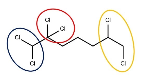
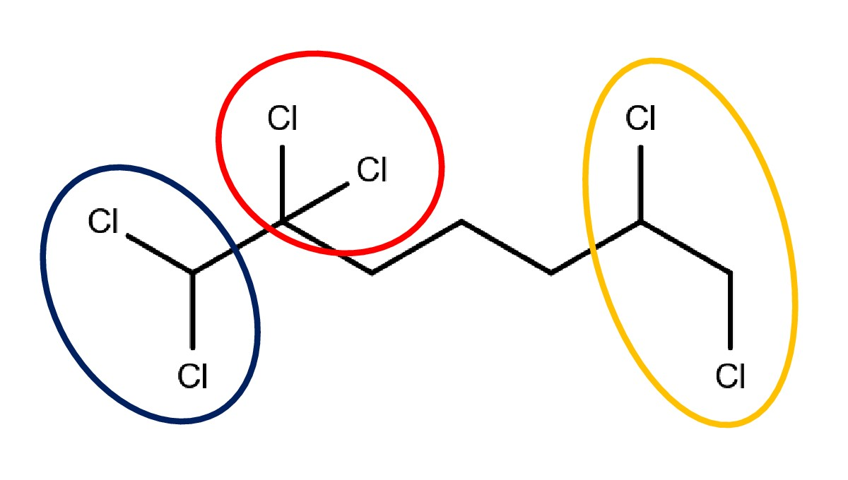
3.1. Chloro Hydrocarbons
+ NCl non-terminal * GC Cl non-terminal
3.2. Fluoro Hydrocarbons
 – CH2 – CH3
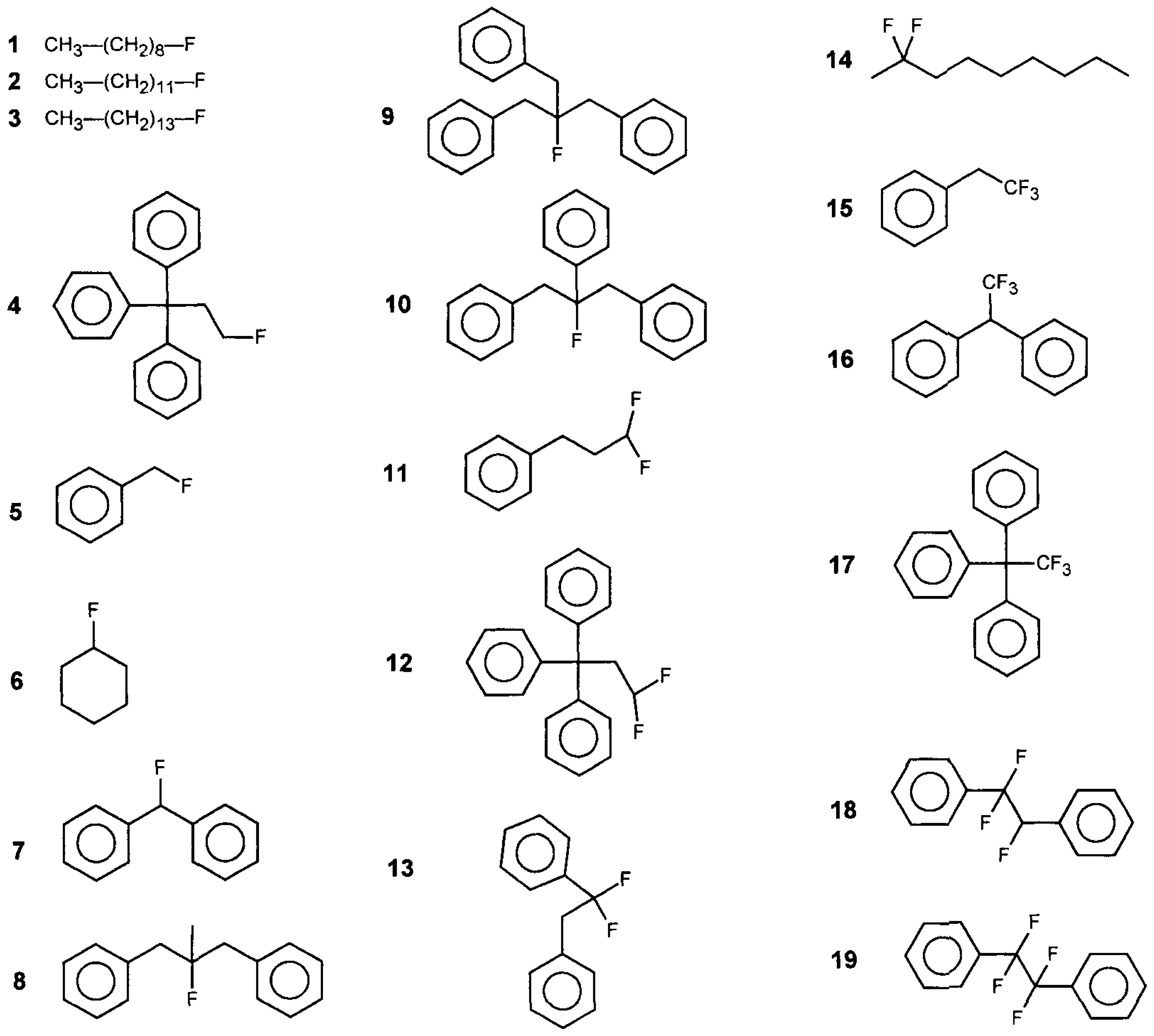
and CH3. Note that whereas in the first case all CH2 are equivalent, in the second case CH2 ≠ CH2 ≠ that now comprises the groups Fterminal, CH2, CH2, and CH3. Note that whereas in the first case all CH2 were equivalent, in the second case, CH2 ≠ CH2 ≠ CH2. Thus, we would need to introduce two further GC parameters. However, for multiple substituted fluoroalkanes, further parameters will be required, and not only for the CH2 but also for the CH and the C group. Whereas this is possible on paper, in practice, we do not have the experimental data to develop this further. Finally, we have now been talking about the fluoroalkanes only, but the same applies to structures involving affected carbon atoms in phenyl rings such as in structures 5, 7, 10, 13, 18, and 19.
– CH2 – CH3
and CH3. Note that whereas in the first case all CH2 are equivalent, in the second case CH2 ≠ CH2 ≠ that now comprises the groups Fterminal, CH2, CH2, and CH3. Note that whereas in the first case all CH2 were equivalent, in the second case, CH2 ≠ CH2 ≠ CH2. Thus, we would need to introduce two further GC parameters. However, for multiple substituted fluoroalkanes, further parameters will be required, and not only for the CH2 but also for the CH and the C group. Whereas this is possible on paper, in practice, we do not have the experimental data to develop this further. Finally, we have now been talking about the fluoroalkanes only, but the same applies to structures involving affected carbon atoms in phenyl rings such as in structures 5, 7, 10, 13, 18, and 19.3.3. Benzylhalides
3.4. Nitro Compounds
3.5. Acetals: 1,3-Dioxolane
 as a group. We can now see from the data in Table 6 that we achieved good agreement between the experimental and our model values for a further eight dioxolanes, with only the value for 2,2-di-iPr-1,3-dioxolane beyond somewhat beyond chemical accuracy. For 2-Me-2-iPr-1,3-dioxolane and 2,2-di-iPr-1,3-dioxolane, we included the Me-Me neighbor interaction parameters as established previously in our work on branched alkanes [11]. The averaged absolute difference between experimental and model values for the eight substituted 1,3-dioxolanes read as 2.50 kJ/mol. On the contrary, the model of Marrero and Gani and the model of Joback and Reid (both implementations in ICSAS23) revealed significant differences between the model and the experimental values.
4. Summary
5. Conclusions and Outlook
Supplementary Materials
Funding
Institutional Review Board Statement
Informed Consent Statement
Data Availability Statement
Acknowledgments
Conflicts of Interest
References
- Van Krevelen, D.W.; Chermin, H.A.G. Estimation of the free enthalpy (Gibbs free energy) of formation of organic compounds from group contributions. Chem. Eng. Sci. 1951, 1, 66–80, Erratum in 1952, 1, 238. [Google Scholar] [CrossRef]
- Benson, S.W.; Cruickshank, F.R.; Golden, D.M.; Haugen, G.R.; O‘Neal, H.E.; Rodgers, A.S.; Shaw, R.; Walsh, R. Additivity rules for the estimation of thermochemical properties. Chem. Rev. 1968, 69, 279–324. [Google Scholar] [CrossRef]
- Cohen, N.; Benson, S. Estimation of the heats of formation of organic compounds. Chem. Rev. 1993, 93, 2419–2438. [Google Scholar] [CrossRef]
- Joback, K.G.; Reid, R.C. Estimation of Pure-Component Properties from Group-Contributions. Chem. Eng. Commun. 1987, 57, 233–243. [Google Scholar] [CrossRef]
- Constantinou, L.; Gani, R. New group contribution method for estimating properties of pure compounds. AIChE J. 1994, 40, 1697–1710. [Google Scholar] [CrossRef]
- Marrero, J.; Gani, R. Group-contribution based estimation of pure component properties. Fluid Phase Equilibria 2001, 183–184, 183–208. [Google Scholar] [CrossRef]
- Hukkerikar, A.S.; Meier, R.J.; Sin, G.; Gani, R. A method to estimate the enthalpy of formation of organic compounds with chemical accuracy. Fluid Phase Equilibria 2013, 348, 23–32. [Google Scholar] [CrossRef]
- Argoub Kadda, A.; Mustapha, B.A.; Yahiaoui, A.; Khaled, T.; Hadji, D. Enthalpy of Formation Modeling Using Third Order Group Contribution Technics and Calculation by DFT Method. Int. J. Thermodyn. (IJoT) 2020, 23, 34–41. [Google Scholar] [CrossRef]
- Aouichaoui, A.R.N.; Fan, F.; Mansouri, S.S.; Abildskov, J.; Sin, G. Molecular Representations in Deep-Learning Models for Chemical Property Prediction. Comput. Aided Chem. Eng. 2022, 49, 1591–1596. [Google Scholar] [CrossRef]
- Meier, R.J. Group contribution revisited: The enthalpy of formation of organic compounds with “chemical accuracy”. ChemEngineering 2021, 5, 24. [Google Scholar] [CrossRef]
- Meier, R.J. Group contribution revisited: The enthalpy of formation of organic compounds with “chemical accuracy” Part II. AppliedChem 2021, 1, 111–129. [Google Scholar] [CrossRef]
- Available online: https://webbook.nist.gov/ (accessed on 20 October 2022).
- Proped (Property Prediction) Module Version 4.7 in ICAS23. Danish Technical University, Kongens Lyngby. Available online: https://www.kt.dtu.dk/english/research/kt-consortium/software (accessed on 20 October 2022).
- Spartan’ 10. Wavefunction Inc., Irvine, CA, USA. Available online: www.wavefun.com (accessed on 20 October 2022).
- Tirado-Rives, J.; Jorgensen, W.L. Performance of B3LYP Density Functional Methods for a Large Set of Organic Molecules. J. Chem. Theory Comput. 2008, 4, 297–306. [Google Scholar] [CrossRef] [PubMed]
- Manion, J.A. Evaluated Enthalpies of Formation of the Stable Closed Shell C1 and C2 Chlorinated Hydrocarbons. J. Phys. Chem. Ref. Data 2002, 31, 123–172. [Google Scholar] [CrossRef] [Green Version]
- Fletcher, R.A.; Pilcher, G. Measurements of heats of combustion by flame calorimetry. Part 7.—Chloromethane, chloroethane, 1-chloropropane, 2-chloropropane. Trans. Faraday Soc. 1971, 67, 3191–3201. [Google Scholar] [CrossRef]
- Stridth, G.; Sunner, S. Enthalpies of formation of some 1-chloroalkanes and the CH2-increment in the 1-chloroalkanes series. J. Chem. Thermodyn. 1975, 7, 161–168. [Google Scholar] [CrossRef]
- He, J.; An, X.; Hu, R. Measurements of enthalpies of formation of 2-chlorobutane and 1,2-dichlorobutane in gaseous state. Acta Chim. Sin. 1992, 50, 961–966. [Google Scholar]
- Lacher, J.R.; Amador, A.; Park, J.D. Reaction heats of organic compounds. Part 5.—Heats of hydrogenation of dichloromethane, 1,1- and 1,2-dichloroethane and 1,2-dichloropropane. Trans. Faraday Soc. 1967, 63, 1608–1611. [Google Scholar] [CrossRef]
- An, X.; He, J.; Hu, R. Study on the electrostatic interaction in organic chlorocompounds. Enthalpies of compustion and formation of 1,3- and 1,4-dichlorobutanes. Thermochim. Acta 1990, 169, 331–337. [Google Scholar]
- Pijpers, A.P.; Meier, R.J. Core Level Photoelectron Spectroscopy for Polymer and Catalyst Characterisation. Chem. Soc. Rev. 1999, 28, 233–238. [Google Scholar] [CrossRef]
- Schaffer, F.; Verevkin, S.P.; Rieger, H.-J.; Beckhaus, H.-D.; Rüchardt, C. Enthalpies of Formation of a Series of Fluorinated Hydrocarbons and Strain-Free Group Increments to Assess Polar and Anomeric Stabilization and Strain. Liebigs Ann. 1997, 1997, 1333–1344. [Google Scholar] [CrossRef]
- Kolesov, V.P.; Papina, T.S. Thermochemistry of Haloethanes. Russ. Chem. Rev. 1983, 52, 425. [Google Scholar] [CrossRef]
- Kormos, B.L.; Liebman, J.F.; Cramer, C.J. 298 K enthalpies of formation of monofluorinated alkanes: Theoretical predictions for methyl, ethyl, isopropyl and tert-butyl fluoride. J. Phys. Org. Chem. 2004, 17, 656–664. [Google Scholar] [CrossRef]
- Verevkin, S.P.; Krasnykh, E.L.; Wright, J.S. Thermodynamic properties of benzyl halides: Enthalpies of formation, strain enthalpies, and carbon–halogen bond dissociation enthalpies. Phys. Chem. Chem. Phys. 2003, 5, 2605–2611. [Google Scholar] [CrossRef]
- Härtel, M.A.C.; Klapötke, T.M.; Emel’yanenko, V.N.; Verevkin, S.P. Aliphatic nitroalkanes: Evaluation of thermochemical data with complementary experimental and computational methods. Thermochim. Acta 2017, 656, 151–160. [Google Scholar] [CrossRef]
- Fritzsche, K.; Dogan, B.; Beckhaus, H.-D.; Rüchardt, C. Geminale substituenteneffekte: Teil I. Thermochemie von 1-nitro-, 2-nitro-, 2,2-dinitro-und 2-cyano-2-nitroadamantan. Thermochim. Acta 1990, 160, 147–159. [Google Scholar] [CrossRef]
- Verevkin, S.P. Improved Benson Increments for the Estimation of Standard Enthalpies of Formation and Enthalpies of Vaporization of Alkyl Ethers, Acetals, Ketals, and Ortho Esters. J. Chem. Eng. Data 2002, 47, 1071–1097. [Google Scholar] [CrossRef]
- Verevkin, S.P.; Konnova, M.E.; Turovtsev, V.V.; Riabchunova, A.V.; Pimerzin, A.A. Weaving a Network of Reliable Thermochemistry around Lignin Building Blocks: Methoxy-Phenols and Methoxy-Benzaldehydes. Ind. Eng. Chem. Res. 2020, 59, 22626–22639. [Google Scholar] [CrossRef]


| Chloromethanes | Manion [16] |
|---|---|
| CH3Cl | −81.9 |
| CH2Cl2 | −95.1 |
| CHCl3 | −102.9 |
| CCl4 | −95.6 |
| Chloroalkanes | Exp. Value | Model dHf | Model-Exp | ABS (Model-Exp) | ABS (MG-Exp) |
|---|---|---|---|---|---|
| Chloroethane (Manion [16]) | −112.1 | −113.49 | −1.39 | 1.39 | 9.30 |
| 1-Chloropropane (Fletcher and Pilcher [17]) | −132 | −134.12 | −2.12 | 2.12 | 0.10 |
| 1-Chlorobutane (Stridth et al. [18]) | −154.6 | −154.75 | −0.15 | 0.15 | 2.00 |
| 1-Chloropentane (Stridth et al. [18]) | −175.2 | −175.38 | −0.18 | 0.18 | 1.90 |
| 1-Chlorooctane (Stridth et al. [18]) | −238.9 | −237.27 | 1.63 | 1.63 | 3.50 |
| 1-Chlorododecane (Stridth et al. [18]) | −322 | −319.79 | 2.21 | 2.21 | 3.90 |
| 2-Chloropropane (Fletcher and Pilcher [17]) | −145 | −145.72 | −0.72 | 0.72 | 0.40 |
| 2-Chlorobutane (He et al. [19]) | −166.7 | −166.35 | 0.35 | 0.35 | 3.30 |
| Averaged absolute difference | 1.09 | 3.05 |
| Dichloroalkanes | Exp. Value | Model dHf | Model-Exp | ABS (Model-Exp) | MG-Exp | Joback and Reid-Exp | Final Model Present Work-Exp |
|---|---|---|---|---|---|---|---|
| 1,1-dichloroethane (Manion [16]) | −132.5 | −147.36 | −14.86 | 14.86 | 0.50 | 11.5 | 1.74 |
| 1,2-dichloroethane (Manion [16]) | −132 | −142.26 | −10.26 | 10.26 | 6.80 | 16 | −4.26 |
| 1,2-dichloropropane (Lacher et al. [20]) | −162.8 | −174.49 | −11.69 | 11.69 | 7.45 | 20.8 | −5.69 |
| 1,2-dichlorobutane (He et al. [19]) | −191.2 | −195.12 | −3.92 | 3.92 | 0.84 | 28.6 | 2.08 |
| 1,3-dichlorobutane (He et al. [21]) | −195 | −195.12 | −0.12 | 0.12 | 4.00 | 32.40 | −0.12 |
| 1,4-dichlorobutane (An et al. [21]) | −183.4 | −183.52 | −0.12 | 0.12 | 3.25 | 26.4 | −0.12 |
| averaged absolute difference | 6.83 | 3.81 | 22.6 | 2.33 | |||
| Tri-, tetra-, hexachlororethane | exp. value [16] | model dHf | model-exp | ABS (model-exp) | MG-exp | Joback and Reid-exp | Final model present work-exp |
| 1,1,1-trichloroethane | −144.6 | −194.86 | −50.26 | 50.26 | 2.3 | 4 | −0.46 |
| 1,1,2-trichloroethane | −148 | −176.13 | −28.13 | 28.13 | 13.00 | 11 | 0.47 |
| 1,1,1,2-tetrachloroethane | −152.3 | −222.63 | −70.33 | 70.33 | 17.70 | −3.7 | −2.53 |
| 1,1,2,2-tetrachloroethane | −156.7 | −210 | −53.30 | 53.3 | 4.70 | −1.3 | 3.90 |
| pentachloroethane | −155.9 | −257.5 | −101.60 | 101.6 | 31.10 | −21.1 | 0.80 |
| hexachloroethane | −148.2 | −305 | −156.80 | 156.8 | 52.80 | −48.4 | −3.20 |
| averaged absolute difference | 76.7 | 20.3 | 14.9 | 1.89 |
| Fluoroalkanes | Exp. Value | Model dHf | Model-Exp | ABS (Model-Exp) + Corr. | ABS (ICAS23-Exp) | Number in [23], See Scheme 1 |
|---|---|---|---|---|---|---|
| Fluoroethane [25] | −278 | −281.49 | −3.49 | 3.49 | 13.60 | |
| 2-Fluoropropane [25] | −315.7 | −317.22 | −1.52 | 1.52 | ||
| 2-Fluoro-2-methylpropane [25] | −360 | −360.58 | −0.58 | 0.58 | ||
| 1-Fluorononane [23] | −423.5 | −425.9 | −2.40 | 2.40 | 14.30 | 1 |
| 1-Fluorododecane [23] | −489.2 | −487.8 | 1.41 | 1.41 | 18.20 | 2 |
| 1-Fluorotetradecane [23] | −533.0 | −529.1 | 3.95 | 3.95 | 20.00 | 3 |
| 2,2-Difluorononane [23] | −671.4 | −674.5 | −3.10 | 3.10 | 14 | |
| (1,3-Diphenyl)-2-methyl-2-fluoropropane [23] | −136.7 | −136.1 | 0.58 | 0.58 | 8 | |
| Fluorocyclohexane [23] | −336.6 | −341.9 | −5.28 | 5.28 | 103.22 | 6 |
| 1,1-Difluoroethane [24] | −497 | −483.36 | 13.64 | 3.86 | 88.40 | |
| 1,1-Difluoro-3-phenyl-propane [23] | −414.4 | −392.9 | 21.5 | 4.0 | 6.04 | 11 |
| 1,1,1-Trifluoroethane [24] | −748.7 | −698.9 | 49.84 | 2.7 | 43.04 | |
| 1-Chloro-1-fluoroethane [24] | −313.4 | −315.36 | −1.96 | 1.96 | 291.96 | |
| Averaged absolute difference | 2.68 | 66.53 | ||||
| 1,1,2-Trifluoroethane [24] | −691 | −659.50 | 31.50 | 0.0 | ||
| 1,1-Diphenyl(fluoromethane) [23] | −42.6 | −55.5 | −12.90 | 12.9 | −69.40 | 7 |
| 1,3-Diphenyl-(2-methylphenyl)2-fluoropropane [23] | −14.1 | −23.9 | −9.8 | 9.8 | 9 | |
| 1,3-Diphenyl-2-phenyl-2-fluoropropane [23] | 15.0 | −3.3 | −18.3 | 18.3 | −42.00 | 10 |
| Fluoromethylbenzene [23] | −126.3 | −148.6 | −22.4 | 22.4 | −64.09 | 5 |
| Trifluoroethylbenzene [23] | −623.9 | −586.6 | 37.2 | 15.3 | 31.32 | 15 |
| 1,1-Diphenyl(trifluoroethane) [23] | −516.1 | −479.5 | 36.6 | 15.9 | 24.42 | 16 |
| Triphenyl(3-fluoropropane) [23] | 57.5 | 10.7 | −46.8 | 46.8 | −10.69 | 4 |
| 1,2-Diphenyl-1,1-difluoroethane [23] | −260.5 | −305.6 | −45.1 | 62.6 | −110.62 | 13 |
| 1,1,1-Triphenyl-3,3-difluoropropane [23] | −157.6 | −191.1 | −33.5 | 51.0 | −31.99 | 12 |
| 1,1,1-Triphenyl-2,2,2-trifluoroethane [23] | −364.9 | −386.0 | −21.1 | 73.6 | −8.85 | 17 |
| 1,2-Diphenyl-1,1,2-trifluoroethane [23] | −462.2 | −521.5 | −59.3 | 90.8 | −169.30 | 18 |
| 1,2-Diphenyl-1,1,2,2-tetrafluoroethane [23] | −689.0 | −751.0 | −62.0 | 125.0 | −195.84 | 19 |
| Nitro Compounds | Exp. [27] | Model dHf | Model-Exp | ABS (Model-Exp) | ABS (Model-Exp + Corr.) |
|---|---|---|---|---|---|
| Mononitrile Alkanes | |||||
| Nitromethane | −71.5 | −80.36 | −8.86 | ||
| Nitroethane | −102.4 | −100.99 | 1.41 | 1.41 | |
| 1-Nitropropane | −124.4 | −121.62 | 2.78 | 2.78 | |
| 2-Nitropropane | −140 | −138.72 | 1.28 | 1.28 | |
| 1-Nitrobutane | −145 | −142.25 | 2.75 | 2.75 | |
| 2-Nitrobutane | −163 | −159.35 | 3.65 | 3.65 | |
| 1-Nitropentane | −165 | −162.88 | 2.12 | 2.12 | |
| 2-Nitrodecane | −278.1 | −283.13 | −5.03 | 5.03 | |
| 1,3-Dinitropropane | −135.5 | −137.89 | −2.39 | 2.39 | |
| 1,4-Dinitrobutane | −155.6 | −158.52 | −2.92 | 2.92 | |
| Nitrocyclohexane | −159.2 | −156.75 | 2.45 | 2.45 | |
| 2-Me-2-nitropropane | −186.1 | −182.28 | 3.82 | 3.82 | |
| Averaged absolute difference | 2.78 | ||||
| 2,4,4-Trimethyl-2-nitropentane | −249.4 | −279.73 | −30.33 | 30.33 | |
| Dinitro alkanes | |||||
| Dinitromethane | −38.4 | −80 | −41.6 | 41.6 | 6.6 |
| 1,1-Dinitroethane | −87.2 | −122.36 | −35.16 | 35.16 | 0.16 |
| 1,1-Dinitropropane | −109.5 | −142.99 | −33.49 | 33.49 | 1.51 |
| 1,1-Dinitrobutane | −132.1 | −163.62 | −31.52 | 31.52 | 3.48 |
| 1,1-Dinitropentane | −147.8 | −184.25 | −36.45 | 36.45 | 1.45 |
| 2,2-Dinitropropane | −135 | −185.72 | −50.72 | 50.72 | |
| 1,2-Dinitroethane | −96.7 | −117.26 | −20.56 | 20.56 | |
| 2,3-Dimethyl-2,3-dinitrobutane | −226.2 | −271.44 | −45.24 | 45.24 |
| 1,3-Dioxolanes | Experimental Value [29] | Model | ABS (Model-Exp) | ABS (ICAS23-Exp) | ABS (Joback and Reid-Exp) |
|---|---|---|---|---|---|
| 1,3-Dioxolane | −301.6 | 0 | 6.2 | 13.2 | |
| 2-Me-1,3-dioxolane | −344.1 | −343.96 | 0.14 | 14.8 | 14.7 |
| 2-nPr-1,3-dioxolane | −386.8 | −385.22 | 1.58 | 11 | 16.1 |
| 2,2-di-Me-1,3-dioxolane | −389.4 | −386.32 | 3.08 | 33.2 | 54.6 |
| 2-Me-2-Et-1,3-dioxolane | −409.7 | −406.95 | 2.75 | 28.9 | 54.2 |
| 2-Me-2-nPr-1,3-dioxolane | −429.2 | −427.58 | 1.62 | 27.8 | 53.1 |
| 2-Me-2-nPe-1,3-dioxolane | −468.8 | −468.84 | 0.04 | 26 | 51.4 |
| 2-Me-2-iPr-1,3-dioxolane | −421.9 | −417.78 | 4.12 | 40.3 | 40.5 |
| 2,2-di-iPr-1,3-dioxolane | −456 | −449.24 | 6.76 | 48.9 | 28.1 |
| Averaged absolute difference | 2.51 | 28.86 | 39.09 |
Publisher’s Note: MDPI stays neutral with regard to jurisdictional claims in published maps and institutional affiliations. |
© 2022 by the author. Licensee MDPI, Basel, Switzerland. This article is an open access article distributed under the terms and conditions of the Creative Commons Attribution (CC BY) license (https://creativecommons.org/licenses/by/4.0/).
Share and Cite
Meier, R.J. Group Contribution Revisited: The Enthalpy of Formation of Organic Compounds with “Chemical Accuracy” Part III. AppliedChem 2022, 2, 213-228. https://doi.org/10.3390/appliedchem2040015
Meier RJ. Group Contribution Revisited: The Enthalpy of Formation of Organic Compounds with “Chemical Accuracy” Part III. AppliedChem. 2022; 2(4):213-228. https://doi.org/10.3390/appliedchem2040015
Chicago/Turabian StyleMeier, Robert J. 2022. "Group Contribution Revisited: The Enthalpy of Formation of Organic Compounds with “Chemical Accuracy” Part III" AppliedChem 2, no. 4: 213-228. https://doi.org/10.3390/appliedchem2040015