Deriving an Electric Wave Equation from Weber’s Electrodynamics

Abstract

Weber’s electrodynamics presents an alternative theory to the widely accepted Maxwell–Lorentz electromagnetism. It is founded on the concept of direct action between particles, and has recently gained some momentum through theoretical and experimental advancements. However, a major criticism remains: the lack of a comprehensive electromagnetic wave equation for free space. Our motivation in this research article is to address this criticism, in some measure, by deriving an electric wave equation from Weber’s electrodynamics based on the axiom of vacuum polarization. Although this assumption has limited experimental evidence and its validity remains a topic of debate among researchers, it has been shown to be useful in the calculation of various quantum mechanical phenomena. Based on this concept, and beginning with Weber’s force, we derive an expression which resembles the familiar electric field wave equation derived from Maxwell’s equations.

1. Introduction

Classic electromagnetism is based on Maxwell’s equations and the Lorentz force. As an alternative to Maxwell–Lorentz electromagnetism, Weber’s electrodynamics can also explain a range of electromagnetic phenomena, but it has received significantly less attention [1,2]. In recent years, progress has been made in both experimental and theoretical research on Weber electrodynamics. A series of new experiments, including electron beam deflections [3,4], electron beam induction [5], the prediction of magnetic force direction within a capacitor [6], and wave-particle duality investigations utilizing a Hertzian dipole acting as a single quantum object [7], have provided evidence supporting the validity of Weber’s electrodynamics. In addition, a six-component force representing Weber’s electrodynamics has been introduced, making calculations simpler for cases involving large numbers of particles [8]. Weber’s electrodynamics has also been extended for the regime of high-velocity particles [9,10], and proposed as a more physically intuitive explanation of Faraday’s paradox [11].

The success of Maxwell’s equations in deriving the electromagnetic wave equation and explaining a range of electromagnetic phenomena is profound and has been well documented. Whilst Maxwell’s equations have been influential in our understanding of electromagnetic waves, it was Weber’s electrodynamics that first established the relationship between the speed of light and electromagnetic waves [2]. Nevertheless, Weber’s electrodynamics has faced criticism for its inability to predict electromagnetic waves in free space, including its failure to explain electromagnetic wave phenomena, such as radar [12] and cold plasma oscillations [13]. However, in the past few decades, researchers have challenged this view and made progress in using Weber’s electrodynamics to explain electromagnetic waves. In particular, Assis [14,15] employed Weber’s electrodynamics to derive a wave equation for signal propagation in conductors, while Wesley [16] derived a wave equation by introducing time retardation into Weber’s electrodynamics. Kühn [17] developed an inhomogeneous wave equation from Maxwell’s equations to be compatible with Weber’s electrodynamics under certain conditions (observer rest frame, charge as a function of velocity, and uniform charge velocity). Interestingly, there is another approach in which the vacuum is not regarded as empty. It is based on the quantum mechanical idea that, under the influence of an external electric field, the vacuum is polarized through the creation of so-called virtual-particle/anti-particle pairs [18,19]. In 2003, Fukai [20] put forward comparable ideas in which electrical signals propagating through a vacuum were hypothesized to have an equivalent circuit consisting of a series of LC components (i.e., inductors and capacitors).

Building on these ideas, herein we assume a polarized vacuum consisting of positive and negative charges and, for the first time, successfully derive an electric wave equation for free space based on the telegraphy ideas of Weber, Kirchoff, and Assis [14,15]. While Maxwell’s equations have undoubtedly been successful in explaining electromagnetic phenomena, recent advancements in Weber’s electrodynamics can potentially offer an intriguing and complementary insight regarding the behavior of electromagnetic waves.

2. Weber’s Electrodynamics

Compared to Maxwell–Lorentz electromagnetism, Weber’s electrodynamics gives a much simpler form for particle–particle interaction forces. For two particles interacting with each other, the force exerted by one particle on the other is given by [21]

$$\stackrel{⃑}{F}=\frac{Qq\widehat{r}}{4\pi {\epsilon }_0{r}^2}\left[1+\frac{1}{c^2}\left(\stackrel{⃑}{v}·\stackrel{⃑}{v}-\frac{3}{2}{\left(\widehat{r}·\stackrel{⃑}{v}\right)}^2+r\widehat{r}·\stackrel{⃑}{a}\right)\right]$$

(1)

where $Q$ and $q$ are two electrical charges, $\stackrel{⃑}{F}$ is the force that charge $Q$ exerted on charge $q$, $r$ is the distance between the two charges, $\widehat{r}$ is the unit vector pointing from charge $Q$ to charge $q$, $\stackrel{⃑}{v}$ and $\stackrel{⃑}{a}$ are the velocity and acceleration of charge $q$ relative to charge $Q$, ${\epsilon }_0$ is the dielectric constant, and $c$ is the speed of light. This force has been used in numerous studies of Weber’s electrodynamics before, e.g., [1,2,3,4,5,6,7,8,9,10,11,14,15,16,17,21]. The symbols used in this paper are listed in

Table 1. List of symbols used in this paper.

Symbol	Meaning	Symbol	Meaning
$\stackrel{⃑}{F}$	Total force.	$Q$, $q$	Electrical charges.
${\stackrel{⃑}{F}}_c$	Integrated static (Coulomb) force.	${\epsilon }_0$	Dielectric constant.
${\stackrel{⃑}{F}}_v$	Integrated velocity related force.	$c$	Speed of light.
${\stackrel{⃑}{F}}_a$	Integrated acceleration related force.	$\widehat{r}$	Unit vector.
$\stackrel{⃑}{f}$	Force between two parcels of charges.	$r$	Distance between the two charges.
${\stackrel{⃑}{f}}_c$	Static (Coulomb) force.	$\stackrel{⃑}{v}$	Relative velocity.
${\stackrel{⃑}{f}}_v$	Velocity related force.	$\stackrel{⃑}{a}$	Relative acceleration.
${\stackrel{⃑}{f}}_a$	Acceleration related force.	$\stackrel{⃑}{E}$	External electric field.
${\stackrel{⃑}{D}}_{+}$,${\stackrel{⃑}{D}}_{-}$	Displacement of positive and negative charges.	$g\left(\right)$	Relationship between the electric field and the displacement field.
${\stackrel{⃑}{v}}_{+}$,${\stackrel{⃑}{v}}_{-}$	Velocity of positive and negative charges.	$\nabla ·$	Divergence operator.
${\stackrel{⃑}{a}}_{+}$,${\stackrel{⃑}{a}}_{-}$	Acceleration of positive and negative charges.	$O\left({\stackrel{⃑}{r}}^2\right)$	Higher-order terms.
${\rho }_{+}$,${\rho }_{-}$	Absolute density of positive and negative charges.	$·$	Dot product of vector.
$\rho$	Average density of positive and negative charges.	$\nabla$	Gradient operator.
${\rho }_{-}\left(\stackrel{⃑}{r}\right)$	Density of negative charge at location $\stackrel{⃑}{r}$. Similar symbol for positive charge.	$dV$	Small parcel at origin.
${\stackrel{⃑}{v}}_{-}\left(\stackrel{⃑}{r}\right)$	Velocity of negative charge at location $\stackrel{⃑}{r}$.	$d\acute{V}$	Small parcel at location $\stackrel{⃑}{r}$ on the shell.
${\stackrel{⃑}{a}}_{-}\left(\stackrel{⃑}{r}\right)$	Acceleration of negative charge at location $\stackrel{⃑}{r}$.	$ds$	Small area on the shell.
${\rho }_{-}\left(\stackrel{⃑}{0}\right)$	Density of negative charge at origin.	$dr$	Thickness of the shell.
${\stackrel{⃑}{v}}_{-}\left(\stackrel{⃑}{0}\right)$	Velocity of negative charge at origin.	$\frac{\partial }{\partial t}$	Eulerian derivative.
${\stackrel{⃑}{a}}_{-}\left(\stackrel{⃑}{0}\right)$	Acceleration of negative charge at origin.	$\frac{d}{dt}$	Lagrangian derivative.
$\chi$	Constant scalar.	$\nabla \times$	Curl operator.
$\mathsf{\Phi }$	Scalar potential.	${\nabla }^2$	Laplacian operator.

below.

The type of force described in Weber’s electrodynamics is often classified as action at a distance (or direct action). The force is exerted instantaneously, regardless of the distance between the interacting particles. Moreover, the force expression (as given in Equation (1)) is relational and can be used to describe the interaction between particles within any reference system.

3. Vacuum Polarization

In this article, in order to derive an electric wave equation from Weber’s force, we postulate that the vacuum behaves similar to a polarizable material. With this assumption, one can then speculate that the vacuum consists of positive and negative charges overlapping each other (Figure 1). These charges can oscillate relative to each other, resulting in a displacement represented by ${\stackrel{⃑}{D}}_{+}$ and ${\stackrel{⃑}{D}}_{-}$ for positive and negative charges, respectively (Equation (2)). When there is no external electric field, the displacement of both positive and negative charges is zero, and the vacuum remains electrically neutral (non-polarized). However, when an external electric field is present, the displacement field becomes non-zero (Equation (2)). As a result, the vacuum may become polarized due to the continuous variation in charge density, which is related to the divergence of the displacement field.

$$\begin{gathered} \begin{array}{c}{\stackrel{⃑}{D}}_{+}=-{\stackrel{⃑}{D}}_{-}\hspace{1em}\hspace{1em}{\stackrel{⃑}{v}}_{+}=-{\stackrel{⃑}{v}}_{-}\hspace{1em}\hspace{1em}{\stackrel{⃑}{a}}_{+}=-{\stackrel{⃑}{a}}_{-}\hfill \\ {\stackrel{⃑}{D}}_{+}=-{\stackrel{⃑}{D}}_{-}=g\left(\stackrel{⃑}{E}\right)\hfill \\ \\ {\rho }_{+}=\rho \left(1-\nabla ·{\stackrel{⃑}{D}}_{+}\right)\hspace{1em}\hspace{1em}{\rho }_{-}=\rho \left(1-\nabla ·{\stackrel{⃑}{D}}_{-}\right)\hspace{1em}\hspace{1em}{\rho }_{+}+{\rho }_{-}=2\rho \hfill \end{array} \end{gathered}$$

(2)

where ${\stackrel{⃑}{D}}_{+}$, ${\stackrel{⃑}{v}}_{+}$, ${\stackrel{⃑}{a}}_{+}$, and ${\rho }_{+}$ are displacement, velocity, acceleration, and density of positive charge, respectively; ${\stackrel{⃑}{D}}_{-}$, ${\stackrel{⃑}{v}}_{-}$, ${\stackrel{⃑}{a}}_{-}$, and ${\rho }_{-}$ are displacement, velocity, acceleration, and density of negative charge, respectively; $\stackrel{⃑}{E}$ is the external electric field; $g\left(\right)$ represents a relationship between the electric field and the displacement field; and $\rho$ is the average density of positive and negative charges. When the density change is small, the formula ${\rho }_{+}=\rho \left(1-\nabla ·{\stackrel{⃑}{D}}_{+}\right)$ is approximated by ${\rho }_{+}=\rho -{\rho }_{+}\nabla ·{\stackrel{⃑}{D}}_{+}$, which is equivalent to the volumetric strain formula in continuum mechanics. Here, the rest frame of the media (positive–negative charge pairs in the vacuum) is used.

4. Derivation of Electric Wave Equation

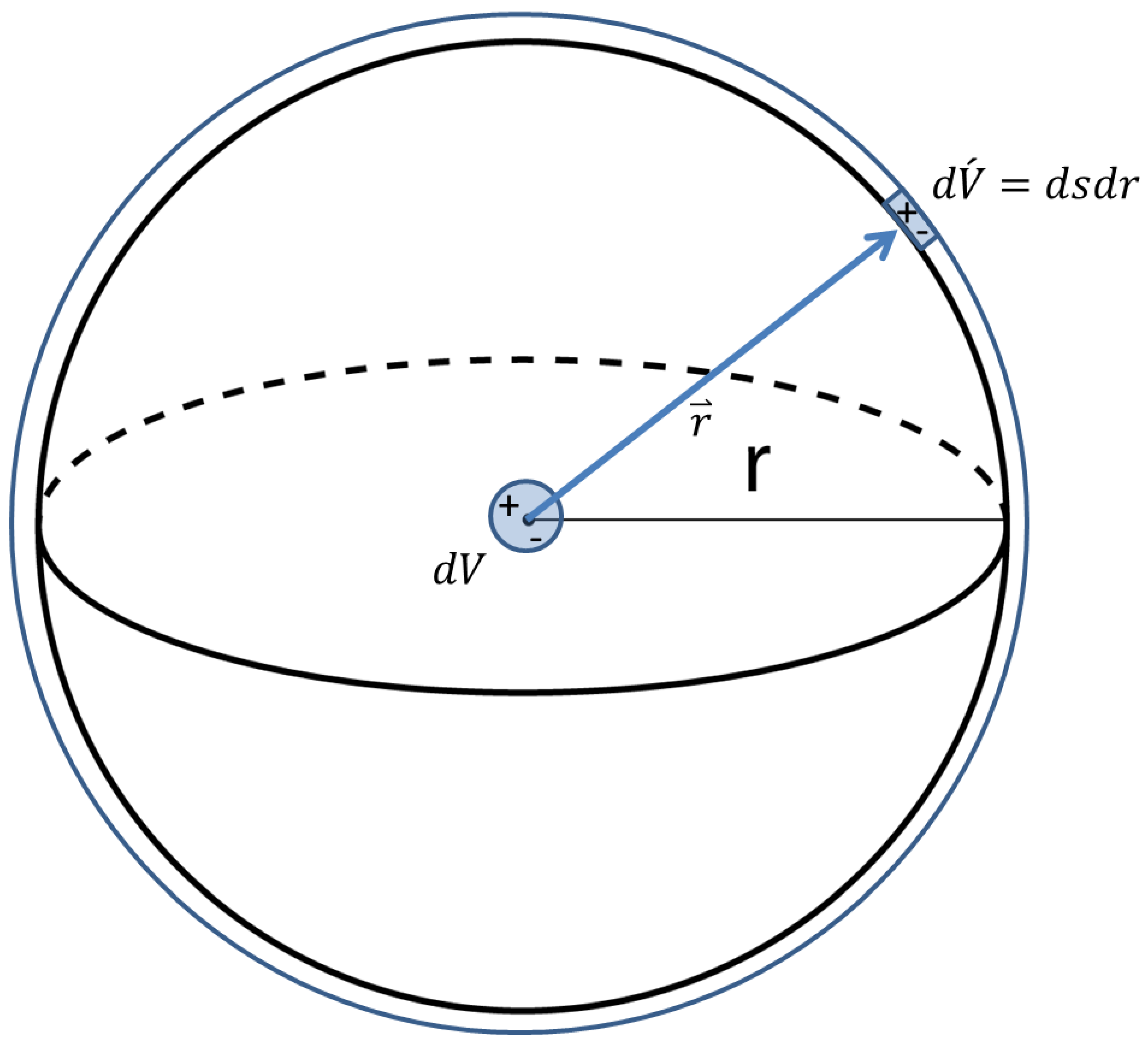
Consider a homogeneous vacuum with positive and negative charges. The negative charge density is ${\rho }_{-}\left(\stackrel{⃑}{r}\right)$, and the velocity and acceleration of negative charge are ${\stackrel{⃑}{v}}_{-}\left(\stackrel{⃑}{r}\right)$ and ${\stackrel{⃑}{a}}_{-}\left(\stackrel{⃑}{r}\right)$, respectively (Figure 2). The density ${\rho }_{+}\left(\stackrel{⃑}{r}\right)$, velocity ${\stackrel{⃑}{v}}_{+}\left(\stackrel{⃑}{r}\right)$, and acceleration ${\stackrel{⃑}{a}}_{+}\left(\stackrel{⃑}{r}\right)$ of positive charge are simply related with those of negative charge (Equation (2)).

Now, apply a Taylor expansion to the quantities of negative and positive charges around the origin, $\stackrel{⃑}{0}$ (Equation (3)). Note that the same expansion applies to positive charge too. The higher-order terms $O\left({\stackrel{⃑}{r}}^2\right)$ will be dropped in the subsequent equation derivations.

$$\begin{gathered} {\rho }_{-}\left(\stackrel{⃑}{r}\right)={\rho }_{-}\left(\stackrel{⃑}{0}\right)+\stackrel{⃑}{r}·\nabla {\rho }_{-}\left(\stackrel{⃑}{0}\right)+O\left({\stackrel{⃑}{r}}^2\right) \\ {\stackrel{⃑}{v}}_{-}\left(\stackrel{⃑}{r}\right)={\stackrel{⃑}{v}}_{-}\left(\stackrel{⃑}{0}\right)+\stackrel{⃑}{r}·\nabla {\stackrel{⃑}{v}}_{-}\left(\stackrel{⃑}{0}\right)+O\left({\stackrel{⃑}{r}}^2\right) \\ {\stackrel{⃑}{a}}_{-}\left(\stackrel{⃑}{r}\right)={\stackrel{⃑}{a}}_{-}\left(\stackrel{⃑}{0}\right)+\stackrel{⃑}{r}·\nabla {\stackrel{⃑}{a}}_{-}\left(\stackrel{⃑}{0}\right)+O\left({\stackrel{⃑}{r}}^2\right) \end{gathered}$$

(3)

Both positive charge ${\rho }_{+}\left(\stackrel{⃑}{r}\right)d\acute{V}$ and negative charge ${\rho }_{-}\left(\stackrel{⃑}{r}\right)d\acute{V}$ on the shell exert force on the negative charge ${\rho }_{-}\left(\stackrel{⃑}{0}\right)dV$ at the origin (Figure 3). Using Weber’s electrodynamics (Equation (1)) and the Taylor expansion of charge quantities (Equation (3)), the combined force $\stackrel{⃑}{f}$ can be written as

$$\begin{array}{ll}\stackrel{⃑}{f}=& \frac{-\stackrel{⃑}{r}}{4\pi {\epsilon }_0{r}^3}{\rho }_{-}\left(\stackrel{⃑}{0}\right)dV{\rho }_{-}\left(\stackrel{⃑}{r}\right)d\acute{V}(1+\frac{1}{c^2}(\left({\stackrel{⃑}{v}}_{-}\left(\stackrel{⃑}{0}\right)+\stackrel{⃑}{r}·\nabla {\stackrel{⃑}{v}}_{-}\left(\stackrel{⃑}{0}\right)-{\stackrel{⃑}{v}}_{-}\left(\stackrel{⃑}{0}\right)\right)·\left({\stackrel{⃑}{v}}_{-}\left(\stackrel{⃑}{0}\right)+\stackrel{⃑}{r}·\nabla {\stackrel{⃑}{v}}_{-}\left(\stackrel{⃑}{0}\right)-{\stackrel{⃑}{v}}_{-}\left(\stackrel{⃑}{0}\right)\right)\\ & -\frac{3}{2r^2}{\left(\stackrel{⃑}{r}·\left({\stackrel{⃑}{v}}_{-}\left(\stackrel{⃑}{0}\right)+\stackrel{⃑}{r}·\nabla {\stackrel{⃑}{v}}_{-}\left(\stackrel{⃑}{0}\right)-{\stackrel{⃑}{v}}_{-}\left(\stackrel{⃑}{0}\right)\right)\right)}^2+\stackrel{⃑}{r}·\left({\stackrel{⃑}{a}}_{-}\left(\stackrel{⃑}{0}\right)+\stackrel{⃑}{r}·\nabla {\stackrel{⃑}{a}}_{-}\left(\stackrel{⃑}{0}\right)-{\stackrel{⃑}{a}}_{-}\left(\stackrel{⃑}{0}\right)\right)\left)\right)\\ & +\frac{\stackrel{⃑}{r}}{4\pi {\epsilon }_0{r}^3}{\rho }_{-}\left(\stackrel{⃑}{0}\right)dV{\rho }_{+}\left(\stackrel{⃑}{r}\right)d\acute{V}(1+\frac{1}{c^2}(\left({\stackrel{⃑}{v}}_{+}\left(\stackrel{⃑}{0}\right)+\stackrel{⃑}{r}·\nabla {\stackrel{⃑}{v}}_{+}\left(\stackrel{⃑}{0}\right)-{\stackrel{⃑}{v}}_{-}\left(\stackrel{⃑}{0}\right)\right)·\left({\stackrel{⃑}{v}}_{+}\left(\stackrel{⃑}{0}\right)+\stackrel{⃑}{r}·\nabla {\stackrel{⃑}{v}}_{+}\left(\stackrel{⃑}{0}\right)-{\stackrel{⃑}{v}}_{-}\left(\stackrel{⃑}{0}\right)\right)\\ & -\frac{3}{2r^2}{\left(\stackrel{⃑}{r}·\left({\stackrel{⃑}{v}}_{+}\left(\stackrel{⃑}{0}\right)+\stackrel{⃑}{r}·\nabla {\stackrel{⃑}{v}}_{+}\left(\stackrel{⃑}{0}\right)-{\stackrel{⃑}{v}}_{-}\left(\stackrel{⃑}{0}\right)\right)\right)}^2+\stackrel{⃑}{r}·\left({\stackrel{⃑}{a}}_{+}\left(\stackrel{⃑}{0}\right)+\stackrel{⃑}{r}·\nabla {\stackrel{⃑}{a}}_{+}\left(\stackrel{⃑}{0}\right)-{\stackrel{⃑}{a}}_{-}\left(\stackrel{⃑}{0}\right)\right)\left)\right)\end{array}$$

(4)

Equation (4) can be broadly separated into two parts, with the first item of the above equation being the force exerted by the negative charge ${\rho }_{-}\left(\stackrel{⃑}{r}\right)d\acute{V}$. The second item is the force exerted by the positive charge ${\rho }_{+}\left(\stackrel{⃑}{r}\right)d\acute{V}$. Overall, the force consists of a static term (Coulomb force), a velocity-related term, and an acceleration-related term.

First, consider the static term (Coulomb force) and use Equations (2) and (3)

$${\stackrel{⃑}{f}}_c=\frac{-\stackrel{⃑}{r}}{4\pi {\epsilon }_0{r}^3}{\rho }_{-}\left(\stackrel{⃑}{0}\right)dV{\rho }_{-}\left(\stackrel{⃑}{r}\right)d\acute{V}+\frac{\stackrel{⃑}{r}}{4\pi {\epsilon }_0{r}^3}{\rho }_{-}\left(\stackrel{⃑}{0}\right)dV{\rho }_{+}\left(\stackrel{⃑}{r}\right)d\acute{V}=\frac{-\stackrel{⃑}{r}}{4\pi {\epsilon }_0{r}^3}{\rho }_{-}\left(\stackrel{⃑}{0}\right)dV\left(2{\rho }_{-}\left(\stackrel{⃑}{0}\right)+2\stackrel{⃑}{r}·\nabla {\rho }_{-}\left(\stackrel{⃑}{0}\right)-2\rho \right)d\acute{V}$$

(5)

Now, integrate around the shell

$${\stackrel{⃑}{F}}_c=-\frac{1}{4\pi {\epsilon }_0{r}^3}{\rho }_{-}\left(\stackrel{⃑}{0}\right)dV\int \left(2{\rho }_{-}\left(\stackrel{⃑}{0}\right)+2\stackrel{⃑}{r}·\nabla {\rho }_{-}\left(\stackrel{⃑}{0}\right)-2\rho \right)\stackrel{⃑}{r}dsdr=-\frac{2r}{3{\epsilon }_0}{\rho }_{-}\left(\stackrel{⃑}{0}\right)dV\nabla {\rho }_{-}\left(\stackrel{⃑}{0}\right)dr$$

(6)

(N.B., further details supporting the integrations carried out in this derivation are included in the Supplementary Information).

Second, consider the velocity-related term

$$\begin{array}{ll}{\stackrel{⃑}{f}}_v=& \frac{-\stackrel{⃑}{r}}{4\pi {\epsilon }_0{r}^3}{\rho }_{-}\left(\stackrel{⃑}{0}\right)dV{\rho }_{-}\left(\stackrel{⃑}{r}\right)d\acute{V}\frac{1}{c^2}(\left({\stackrel{⃑}{v}}_{-}\left(\stackrel{⃑}{0}\right)+\stackrel{⃑}{r}·\nabla {\stackrel{⃑}{v}}_{-}\left(\stackrel{⃑}{0}\right)-{\stackrel{⃑}{v}}_{-}\left(\stackrel{⃑}{0}\right)\right)·\left({\stackrel{⃑}{v}}_{-}\left(\stackrel{⃑}{0}\right)+\stackrel{⃑}{r}·\nabla {\stackrel{⃑}{v}}_{-}\left(\stackrel{⃑}{0}\right)-{\stackrel{⃑}{v}}_{-}\left(\stackrel{⃑}{0}\right)\right)\\ & -\frac{3}{2r^2}{\left(\stackrel{⃑}{r}·\left({\stackrel{⃑}{v}}_{-}\left(\stackrel{⃑}{0}\right)+\stackrel{⃑}{r}·\nabla {\stackrel{⃑}{v}}_{-}\left(\stackrel{⃑}{0}\right)-{\stackrel{⃑}{v}}_{-}\left(\stackrel{⃑}{0}\right)\right)\right)}^2)\\ & +\frac{\stackrel{⃑}{r}}{4\pi {\epsilon }_0{r}^3}{\rho }_{-}\left(\stackrel{⃑}{0}\right)dV{\rho }_{+}\left(\stackrel{⃑}{r}\right)d\acute{V}\frac{1}{c^2}(\left({\stackrel{⃑}{v}}_{+}\left(\stackrel{⃑}{0}\right)+\stackrel{⃑}{r}·\nabla {\stackrel{⃑}{v}}_{+}\left(\stackrel{⃑}{0}\right)-{\stackrel{⃑}{v}}_{-}\left(\stackrel{⃑}{0}\right)\right)\left({\stackrel{⃑}{v}}_{+}\left(\stackrel{⃑}{0}\right)+\stackrel{⃑}{r}·\nabla {\stackrel{⃑}{v}}_{+}\left(\stackrel{⃑}{0}\right)-{\stackrel{⃑}{v}}_{-}\left(\stackrel{⃑}{0}\right)\right)\\ & -\frac{3}{2r^2}{\left(\stackrel{⃑}{r}·\left({\stackrel{⃑}{v}}_{+}\left(\stackrel{⃑}{0}\right)+\stackrel{⃑}{r}·\nabla {\stackrel{⃑}{v}}_{+}\left(\stackrel{⃑}{0}\right)-{\stackrel{⃑}{v}}_{-}\left(\stackrel{⃑}{0}\right)\right)\right)}^2)\end{array}$$

(7)

From Equations (2) and (3), we can have

$$\begin{gathered} {\rho }_{-}\left(\stackrel{⃑}{r}\right)\approx {\rho }_{-}\left(\stackrel{⃑}{0}\right)+\stackrel{⃑}{r}·\nabla {\rho }_{-}\left(\stackrel{⃑}{0}\right) \\ {\rho }_{+}\left(\stackrel{⃑}{r}\right)=2\rho -{\rho }_{-}\left(\stackrel{⃑}{r}\right)\approx 2\rho -{\rho }_{-}\left(\stackrel{⃑}{0}\right)-\stackrel{⃑}{r}·\nabla {\rho }_{-}\left(\stackrel{⃑}{0}\right) \\ {\stackrel{⃑}{v}}_{+}\left(\stackrel{⃑}{0}\right)=-{\stackrel{⃑}{v}}_{-}\left(\stackrel{⃑}{0}\right)\hspace{1em}\hspace{1em}\nabla {\stackrel{⃑}{v}}_{+}\left(\stackrel{⃑}{0}\right)=-\nabla {\stackrel{⃑}{v}}_{-}\left(\stackrel{⃑}{0}\right) \end{gathered}$$

(8)

Inserting Equation (8) into Equation (7), with some simplification we obtain

$$\begin{array}{ll}{\stackrel{⃑}{f}}_v=& \frac{-\stackrel{⃑}{r}}{4\pi {\epsilon }_0{r}^3}{\rho }_{-}\left(\stackrel{⃑}{0}\right)dV\left({\rho }_{-}\left(\stackrel{⃑}{0}\right)+\stackrel{⃑}{r}·\nabla {\rho }_{-}\left(\stackrel{⃑}{0}\right)\right)d\acute{V}\frac{1}{c^2}\left(\left(\stackrel{⃑}{r}·\nabla {\stackrel{⃑}{v}}_{-}\left(\stackrel{⃑}{0}\right)\right)·\left(\stackrel{⃑}{r}·\nabla {\stackrel{⃑}{v}}_{-}\left(\stackrel{⃑}{0}\right)\right)-\frac{3}{2r^2}{\left(\stackrel{⃑}{r}·\left(\stackrel{⃑}{r}·\nabla {\stackrel{⃑}{v}}_{-}\left(\stackrel{⃑}{0}\right)\right)\right)}^2\right)\\ & +\frac{\stackrel{⃑}{r}}{4\pi {\epsilon }_0{r}^3}{\rho }_{-}\left(\stackrel{⃑}{0}\right)dV\left(2\rho -{\rho }_{-}\left(\stackrel{⃑}{0}\right)-\stackrel{⃑}{r}·\nabla {\rho }_{-}\left(\stackrel{⃑}{0}\right)\right)d\acute{V}\frac{1}{c^2}(\left(2{\stackrel{⃑}{v}}_{-}\left(\stackrel{⃑}{0}\right)+\stackrel{⃑}{r}·\nabla {\stackrel{⃑}{v}}_{-}\left(\stackrel{⃑}{0}\right)\right)\\ & ·\left(2{\stackrel{⃑}{v}}_{-}\left(\stackrel{⃑}{0}\right)+\stackrel{⃑}{r}·\nabla {\stackrel{⃑}{v}}_{-}\left(\stackrel{⃑}{0}\right)\right)-\frac{3}{2r^2}{\left(\stackrel{⃑}{r}·\left(2{\stackrel{⃑}{v}}_{-}\left(\stackrel{⃑}{0}\right)+\stackrel{⃑}{r}·\nabla {\stackrel{⃑}{v}}_{-}\left(\stackrel{⃑}{0}\right)\right)\right)}^2)\end{array}$$

(9)

We can then integrate around the shell and drop those higher-order terms which consist of a product of $\stackrel{⃑}{r}·\nabla {\rho }_{-}\left(\stackrel{⃑}{0}\right)$ and $\stackrel{⃑}{r}·\nabla {\stackrel{⃑}{v}}_{-}\left(\stackrel{⃑}{0}\right)$. Thus, we can obtain Equation (10),

$$\begin{array}{cc}{\stackrel{⃑}{F}}_v=\hfill & -\frac{1}{4\pi {\epsilon }_0{r}^3}{\rho }_{-}\left(\stackrel{⃑}{0}\right)dV\int \frac{1}{c^2}\left(\left(\stackrel{⃑}{r}·\nabla {\stackrel{⃑}{v}}_{-}\left(\stackrel{⃑}{0}\right)\right)·\left(\stackrel{⃑}{r}·\nabla {\stackrel{⃑}{v}}_{-}\left(\stackrel{⃑}{0}\right)\right)-\frac{3}{2r^2}{\left(\stackrel{⃑}{r}·\left(\stackrel{⃑}{r}·\nabla {\stackrel{⃑}{v}}_{-}\left(\stackrel{⃑}{0}\right)\right)\right)}^2\right)\left({\rho }_{-}\left(\stackrel{⃑}{0}\right)+\stackrel{⃑}{r}·\nabla {\rho }_{-}\left(\stackrel{⃑}{0}\right)\right)\stackrel{⃑}{r}dsdr\hfill \\ \hfill & +\frac{1}{4\pi {\epsilon }_0{r}^3}{\rho }_{-}\left(\stackrel{⃑}{0}\right)dV\int \frac{1}{c^2}(\left(2{\stackrel{⃑}{v}}_{-}\left(\stackrel{⃑}{0}\right)+\stackrel{⃑}{r}·\nabla {\stackrel{⃑}{v}}_{-}\left(\stackrel{⃑}{0}\right)\right)·\left(2{\stackrel{⃑}{v}}_{-}\left(\stackrel{⃑}{0}\right)+\stackrel{⃑}{r}·\nabla {\stackrel{⃑}{v}}_{-}\left(\stackrel{⃑}{0}\right)\right)\hfill \\ \hfill & -\frac{3}{2r^2}{\left(\stackrel{⃑}{r}·\left(2{\stackrel{⃑}{v}}_{-}\left(\stackrel{⃑}{0}\right)+\stackrel{⃑}{r}·\nabla {\stackrel{⃑}{v}}_{-}\left(\stackrel{⃑}{0}\right)\right)\right)}^2\left)\right(2\rho -{\rho }_{-}\left(\stackrel{⃑}{0}\right)-\stackrel{⃑}{r}·\nabla {\rho }_{-}\left(\stackrel{⃑}{0}\right))\stackrel{⃑}{r}dsdr\hfill \\ \hfill & =-\frac{14r}{15{\epsilon }_0}{\rho }_{-}\left(\stackrel{⃑}{0}\right)dV\frac{1}{c^2}\left({\stackrel{⃑}{v}}_{-}\left(\stackrel{⃑}{0}\right)·{\stackrel{⃑}{v}}_{-}\left(\stackrel{⃑}{0}\right)\right)\nabla {\rho }_{-}\left(\stackrel{⃑}{0}\right)dr+\frac{4r}{5{\epsilon }_0}{\rho }_{-}\left(\stackrel{⃑}{0}\right)dV\frac{1}{c^2}\left({\stackrel{⃑}{v}}_{-}\left(\stackrel{⃑}{0}\right)·\nabla {\rho }_{-}\left(\stackrel{⃑}{0}\right)\right){\stackrel{⃑}{v}}_{-}\left(\stackrel{⃑}{0}\right)dr\hfill \end{array}$$

(10)

Third, consider the acceleration-related term

$$\begin{array}{ll}{\stackrel{⃑}{f}}_a=& \frac{-\stackrel{⃑}{r}}{4\pi {\epsilon }_0{r}^3}{\rho }_{-}\left(\stackrel{⃑}{0}\right)dV{\rho }_{-}\left(\stackrel{⃑}{r}\right)d\acute{V}\frac{1}{c^2}\stackrel{⃑}{r}·\left({\stackrel{⃑}{a}}_{-}\left(\stackrel{⃑}{0}\right)+\stackrel{⃑}{r}·\nabla {\stackrel{⃑}{a}}_{-}\left(\stackrel{⃑}{0}\right)-{\stackrel{⃑}{a}}_{-}\left(\stackrel{⃑}{0}\right)\right)\\ & +\frac{\stackrel{⃑}{r}}{4\pi {\epsilon }_0{r}^3}{\rho }_{-}\left(\stackrel{⃑}{0}\right)dV{\rho }_{+}\left(\stackrel{⃑}{r}\right)d\acute{V}\frac{1}{c^2}\stackrel{⃑}{r}·\left({\stackrel{⃑}{a}}_{+}\left(\stackrel{⃑}{0}\right)+\stackrel{⃑}{r}·\nabla {\stackrel{⃑}{a}}_{+}\left(\stackrel{⃑}{0}\right)-{\stackrel{⃑}{a}}_{-}\left(\stackrel{⃑}{0}\right)\right)\end{array}$$

(11)

From Equations (2) and (3), we obtain

$${\stackrel{⃑}{a}}_{+}\left(\stackrel{⃑}{0}\right)=-{\stackrel{⃑}{a}}_{-}\left(\stackrel{⃑}{0}\right)\hspace{1em}\hspace{1em}\nabla {\stackrel{⃑}{a}}_{+}\left(\stackrel{⃑}{0}\right)=-\nabla {\stackrel{⃑}{a}}_{-}\left(\stackrel{⃑}{0}\right)$$

(12)

Inserting Equation (12) into Equation (11), we obtain

$${\stackrel{⃑}{f}}_a=\frac{-\stackrel{⃑}{r}}{4\pi {\epsilon }_0{r}^3}{\rho }_{-}\left(\stackrel{⃑}{0}\right)dV2\rho d\acute{V}\frac{1}{c^2}\stackrel{⃑}{r}·\left(\stackrel{⃑}{r}·\nabla {\stackrel{⃑}{a}}_{-}\left(\stackrel{⃑}{0}\right)\right)-\frac{\stackrel{⃑}{r}}{4\pi {\epsilon }_0{r}^3}{\rho }_{-}\left(\stackrel{⃑}{0}\right)dV\left({\rho }_{+}\left(\stackrel{⃑}{0}\right)+\stackrel{⃑}{r}·\nabla {\rho }_{+}\left(\stackrel{⃑}{0}\right)\right)d\acute{V}\frac{1}{c^2}\stackrel{⃑}{r}·2{\stackrel{⃑}{a}}_{-}\left(\stackrel{⃑}{0}\right)$$

(13)

Again, we can integrate around the shell and drop the higher-order terms which have a product of $\stackrel{⃑}{r}·\nabla {\rho }_{+}\left(\stackrel{⃑}{0}\right)$ and $\stackrel{⃑}{r}·2{\stackrel{⃑}{a}}_{-}\left(\stackrel{⃑}{0}\right)$. We can also use the approximation ${\rho }_{+}\left(0\right)\approx \rho$.

$$\begin{array}{cc}{\stackrel{⃑}{F}}_a=\hfill & -\frac{1}{4\pi {\epsilon }_0{r}^3}{\rho }_{-}\left(\stackrel{⃑}{0}\right)dV\int \frac{2\rho }{c^2}\stackrel{⃑}{r}·\left(\stackrel{⃑}{r}·\nabla {\stackrel{⃑}{a}}_{-}\left(\stackrel{⃑}{0}\right)\right)\stackrel{⃑}{r}dsdr\hfill \\ \hfill & -\frac{1}{4\pi {\epsilon }_0{r}^3}{\rho }_{-}\left(\stackrel{⃑}{0}\right)dV\int \frac{2}{c^2}\left({\rho }_{+}\left(\stackrel{⃑}{0}\right)+\stackrel{⃑}{r}·\nabla {\rho }_{+}\left(\stackrel{⃑}{0}\right)\right)\stackrel{⃑}{r}·{\stackrel{⃑}{a}}_{-}\left(\stackrel{⃑}{0}\right)\stackrel{⃑}{r}dsdr=-\frac{2r}{3{\epsilon }_0}{\rho }_{-}\left(\stackrel{⃑}{0}\right)dV\frac{\rho }{c^2}{\stackrel{⃑}{a}}_{-}\left(\stackrel{⃑}{0}\right)dr\hfill \end{array}$$

(14)

The total force on negative charge in $dV$ exerted by the shell is

$$\stackrel{⃑}{F}={\stackrel{⃑}{F}}_c+{\stackrel{⃑}{F}}_v+{\stackrel{⃑}{F}}_a$$

(15)

Inserting Equations (6), (10), and (14) into Equation (15), we obtain

$$\begin{array}{cc}\stackrel{⃑}{F}=\hfill & -\frac{2r}{3{\epsilon }_0}{\rho }_{-}\left(\stackrel{⃑}{0}\right)dV\nabla {\rho }_{-}\left(\stackrel{⃑}{0}\right)dr-\frac{14r}{15{\epsilon }_0}{\rho }_{-}\left(\stackrel{⃑}{0}\right)dV\frac{1}{c^2}\left({\stackrel{⃑}{v}}_{-}\left(\stackrel{⃑}{0}\right)·{\stackrel{⃑}{v}}_{-}\left(\stackrel{⃑}{0}\right)\right)\nabla {\rho }_{-}\left(\stackrel{⃑}{0}\right)dr\hfill \\ \hfill & +\frac{4r}{5{\epsilon }_0}{\rho }_{-}\left(\stackrel{⃑}{0}\right)dV\frac{1}{c^2}\left({\stackrel{⃑}{v}}_{-}\left(\stackrel{⃑}{0}\right)·\nabla {\rho }_{-}\left(\stackrel{⃑}{0}\right)\right){\stackrel{⃑}{v}}_{-}\left(\stackrel{⃑}{0}\right)dr-\frac{2r}{3{\epsilon }_0}{\rho }_{-}\left(\stackrel{⃑}{0}\right)dV\frac{\rho }{c^2}{\stackrel{⃑}{a}}_{-}\left(\stackrel{⃑}{0}\right)dr\hfill \end{array}$$

(16)

Since the mass of positive–negative charges in vacuum is likely much smaller compared to that of physical particles, we may choose to ignore their mass and acceleration force in the volume element $dV$. Additionally, the polarization force within a positive–negative charge pair may also be neglected since it is likely small compared to the force exerted by the nearby volume of charges. Equation (16) is valid for a small radius $r$, as we used a Taylor expansion (Equation (3)). Without integrating along the radius $r$, we can set the total force in Equation (16) equal to zero due to force balance. With some simplification, we obtain

$$\nabla {\rho }_{-}\left(\stackrel{⃑}{0}\right)+\frac{7}{5}\frac{1}{c^2}\left({\stackrel{⃑}{v}}_{-}\left(\stackrel{⃑}{0}\right)·{\stackrel{⃑}{v}}_{-}\left(\stackrel{⃑}{0}\right)\right)\nabla {\rho }_{-}\left(\stackrel{⃑}{0}\right)-\frac{6}{5}\frac{1}{c^2}\left({\stackrel{⃑}{v}}_{-}\left(\stackrel{⃑}{0}\right)·\nabla {\rho }_{-}\left(\stackrel{⃑}{0}\right)\right){\stackrel{⃑}{v}}_{-}\left(\stackrel{⃑}{0}\right)+\frac{\rho }{c^2}{\stackrel{⃑}{a}}_{-}\left(\stackrel{⃑}{0}\right)=0$$

(17)

When velocity ${\stackrel{⃑}{v}}_{-}\left(\stackrel{⃑}{0}\right)$ is much less than $c$, we can neglect the velocity-related term. Thus

$$\nabla {\rho }_{-}\left(\stackrel{⃑}{0}\right)+\frac{\rho }{c^2}{\stackrel{⃑}{a}}_{-}\left(\stackrel{⃑}{0}\right)=0$$

(18)

The above equation can also be written as

$$\nabla {\rho }_{-}\left(\stackrel{⃑}{0}\right)+\frac{\rho }{c^2}\frac{d{\stackrel{⃑}{v}}_{-}\left(\stackrel{⃑}{0}\right)}{dt}=0$$

(19)

This expression holds for points other than the origin. Additionally, since ${\stackrel{⃑}{v}}_{-}\left(\stackrel{⃑}{0}\right)$ is small, the Lagrangian derivative can be approximated as a Eulerian derivative. Thus, we can write

$$\nabla {\rho }_{-}+\frac{\rho }{c^2}\frac{\partial {\stackrel{⃑}{v}}_{-}}{\partial t}=0$$

(20)

By applying divergence to the above equation

$$\nabla ·\nabla {\rho }_{-}+\frac{\rho }{c^2}\frac{\partial \left(\nabla ·{\stackrel{⃑}{v}}_{-}\right)}{\partial t}=0$$

(21)

From Equation (2), we have ${\rho }_{-}=\rho \left(1-\nabla ·{\stackrel{⃑}{D}}_{-}\right)$. Applying a time derivative to it, we obtain

$$\frac{\partial {\rho }_{-}}{\partial t}=-\rho \nabla ·\frac{\partial {\stackrel{⃑}{D}}_{-}}{\partial t}=-\rho \nabla ·{\stackrel{⃑}{v}}_{-}$$

(22)

By inserting Equation (22) into Equation (21), we obtain

$$\nabla ·\nabla {\rho }_{-}-\frac{1}{c^2}\frac{{\partial }^2{\rho }_{-}}{\partial t^2}=0$$

(23)

which represents the wave propagation equation for negative charge density.

Next, we can insert equation ${\rho }_{-}=\rho \left(1-\nabla ·{\stackrel{⃑}{D}}_{-}\right)$ into Equation (20), assuming a homogenous vacuum and constant charge density, $\rho$. This gives us

$$-\rho \nabla \nabla ·{\stackrel{⃑}{D}}_{-}+\frac{\rho }{c^2}\frac{\partial {\stackrel{⃑}{v}}_{-}}{\partial t}=0$$

(24)

which can be simplified to

$$-\nabla \nabla ·{\stackrel{⃑}{D}}_{-}+\frac{1}{c^2}\frac{{\partial }^2{\stackrel{⃑}{D}}_{-}}{\partial t^2}=0$$

(25)

Using the vector formula, $\nabla \nabla ·{\stackrel{⃑}{D}}_{-}=\nabla \times \nabla \times {\stackrel{⃑}{D}}_{-}+{\nabla }^2{\stackrel{⃑}{D}}_{-}$, we can simplify Equation (25) further to obtain

$$\nabla \times \nabla \times {\stackrel{⃑}{D}}_{-}+{\nabla }^2{\stackrel{⃑}{D}}_{-}=\frac{1}{c^2}\frac{{\partial }^2{\stackrel{⃑}{D}}_{-}}{\partial t^2}$$

(26)

At first glance, this equation appears a little complex. Therefore, considering a simple scenario of irrotational field ${\stackrel{⃑}{D}}_{-}$ ($\nabla \times \nabla \times {\stackrel{⃑}{D}}_{-}=0$), we obtain

$${\nabla }^2{\stackrel{⃑}{D}}_{-}=\frac{1}{c^2}\frac{{\partial }^2{\stackrel{⃑}{D}}_{-}}{\partial t^2}$$

(27)

Further, we can assume the vacuum is a homogeneous, linear, non-dispersive, and isotropic dielectric medium. We may use a simple expression of vacuum polarization ${\stackrel{⃑}{D}}_{+}=-{\stackrel{⃑}{D}}_{-}=\chi {\epsilon }_0\stackrel{⃑}{E}$, where $\chi$ is a constant scalar; this expression is similar to that of a typical isotropic dielectric medium [22]. Finally, we obtain

$${\nabla }^2\stackrel{⃑}{E}=\frac{1}{c^2}\frac{{\partial }^2\stackrel{⃑}{E}}{\partial t^2}$$

(28)

The equation presented above (28) bears remarkable resemblance to the widely recognized electric field wave equation derived from Maxwell’s equations. For the derivation herein, we start with the balance of Weber’s force, which leads us to the wave equation of the charge displacement field, and, subsequently, we arrive at the wave equation of the electric field. It is important to note that Weber’s force, which arises from the interactions among charges, determines the displacement field. Furthermore, this force can generally be represented by an electric field [8]. In this context, it is worth highlighting that the displacement field is merely a manifestation or an indicator of the electric field.

5. Longitudinal Electric Wave

Longitudinal electric waves travel in the same direction as the electric field. While they have been observed in plasmas [23] and focused beams [24], their existence in free space has been a topic of debate. According to Gauss’s law, the divergence of the electric field in free space must be zero, which implies that the plane or spherical longitudinal waves cannot exist in free space [25]. However, there have been reports of longitudinal electric waves in free space, such as during the eclipse of the sun by the moon [26] and in experiments with spherical antennas [27,28]. To explain these observations, Monstein and Wesley proposed an inhomogeneous wave equation for the scalar potential using Coulomb’s law and time retardation [27]. For clarity, the wave equation is transcribed below (Equation (29)):

$${\nabla }^2\mathsf{\Phi }-\frac{{\partial }^2{\mathsf{\Phi }}^2}{{\partial }^2{t}^2}=-4\pi \rho$$

(29)

where $\mathsf{\Phi }$ is the scalar potential and $\rho$ is the source charge density. Since introducing the time retardation term $\frac{{\partial }^2{\mathsf{\Phi }}^2}{{\partial }^2{t}^2}$, the above equation does not obey Gauss’s law in free space. A similar theory was used to explain longitudinal electric waves in vacuum radiated by an electric dipole [29].

The wave equation derived in this paper does not rely on Gauss’s law. Instead, it is based on the non-zero divergence of electric displacement (and/or electric field). If the divergence is zero, the field will be static and there will be no wave propagation (Equation (25)). Therefore, the theory developed in this paper is compatible with the phenomenon of longitudinal waves and with the theory proposed by Monstein and Wesley.

6. Discussion

This paper posits that the vacuum is not ‘empty’, but rather filled with positive–negative charge pairs. This postulation is not without precedent, as it is somewhat in line with the concept of vacuum polarization in quantum mechanics [18,19], and the Casimir effect of the void [30]. However, it is important to note that there is a fundamental difference between the vacuum postulate in this paper, which has speculated regarding the existence of physical charges in the vacuum, and the quantum mechanical assumption that virtual particle–anti-particle pairs are created in the vacuum.

The Michelson–Morley experiment has long been cited as evidence against the existence of aether or any other free-space medium. However, in this paper, a hypothetical situation is described whereby the vacuum serves as a medium, consisting of positive–negative charge pairs. By considering the rest frame of this medium and assuming small charge velocity, the Lagrangian derivative is approximated as a Eulerian derivative, as shown in Equations (19) and (20). Notably, the wave equation derived herein does not include any sources. Further research should investigate how to incorporate sources and consider cases with varying source and medium velocities. It is also possible that the wave equation derived here may only be valid for stationary media, and further work is needed to explore its limitations and applicability in more general cases.

A criticism that has long been levelled at Weber’s electrodynamics is its supposed incompatibility with fields and electromagnetic waves, since Weber’s force is based on direct action and thus is not conceptually dependent upon fields. Some, such as O’Rahilly, consider that the field is a merely a ‘metaphor’ and that force formulae are the ultimate element of ‘scientific description’ [2]. Nevertheless, even though the literature is heavily weighted towards the idea of fields (electric and magnetic fields), with little consideration for the more fundamental entity of force, Weber’s electrodynamics is remarkably compatible with field theory [17]. It has been shown that the force law of Weber is consistent with Maxwell’s equations [2], and it can be generalized in such a way that its interpretation is based on the concept of fields [2].

It can be said that Maxwell’s equations possess a form of beauty, and the manifestation of the speed of light from the electric and magnetic wave equations, in relation to permittivity and permeability, is masterful. Yet, Maxwell introduced this concept with regard to his displacement current, based on the electrodynamics of Weber. This quantity was first hypothesized by Weber in his force law, which he was also the first to measure (in collaboration Kohlrausch), and, furthermore, along with Kirchoff (independently and at approximately the same time), he was the first to deduce that signals within an electrical circuit would propagate at light velocity based on his force law [14]. Whilst Weber’s electrodynamics has received comparably little/no attention, the derivation herein shows that with certain assumptions, it is possible to obtain an expression that resembles the wave equation for the electric field in free space associated with Maxwell’s equations from Weber’s force.

It is noteworthy that the wave equation for an electric field derived herein (Equation (28)) employs a simple polarization expression ${\stackrel{⃑}{D}}_{+}=-{\stackrel{⃑}{D}}_{-}=\chi {\epsilon }_0\stackrel{⃑}{E}$. However, Weber’s electrodynamics has been shown to consist of six components [8]. Deriving the wave equation for all six components would require further research and a more sophisticated polarization expression that takes into account the relative displacement, velocity, and acceleration of positive–negative charge pairs.

It should also be noted that the wave equation derived in this paper is based on further assumptions and approximations additional to those already discussed. For instance, we neglected higher-order terms, acceleration force, polarization force, and velocity terms, among others. These assumptions and approximations determine the range of applicability of our derivation. Our approach specifically applies to homogeneous vacuum and is most suitable for scenarios involving low relative speeds of charge pairs. Future research is needed to extend to cases when charged particles, such as electrons, exist in the vacuum, and to cases when charge pairs have high relative speeds. Such investigations may require more sophisticated theoretical and mathematical tools.

While the wave equation derived under the assumption of a zero curl (Equation (26)) shares similarities with the widely recognized electric wave equation from Maxwell’s equations, it remains uncertain whether the curl term is always zero. Most likely, it is not, leading to differences with the electromagnetic wave equation associated with Maxwell’s equations. Future research is needed to explore how this equation can be solved to explain electric wave phenomena. Interestingly though, this equation has some similarity to fluid dynamics equations. The curl term may indicate vortex structures in the electric field, akin to those seen in fluids. For instance, ball lightning, a rare and unexplained luminescent spherical object phenomenon [31], may be a potential candidate to study vortex structures in electric fields.

7. Conclusions

A wave equation for the electric field has been successfully derived from Weber’s force, which is also compatible with longitudinal waves. This demonstrates that Weber’s electrodynamics can yield an electric field wave equation for free space, similar to that derived from Maxwell’s equations. However, we speculate that the vacuum is not ‘empty’, but rather it is filled with positive–negative charge pairs, providing the medium for wave propagation. It is important to note that this derivation is based on certain assumptions and approximations which determine its validity and range of applicability, in particular, the hypothetical assumption of charged particle pairs in the vacuum. This idea has some semblance to the concept of vacuum polarization, but the postulation in this paper is somewhat different from the quantum mechanical assumption that virtual particle–anti-particle pairs are created in the vacuum. The electric wave equation derived from Weber’s electrodynamics demonstrates the potential of a Weber-type theory in predicting electromagnetic waves for free space and offers the advantage of dealing only with electrical forces between charges, avoiding magnetic fields, displacement currents, and the like.