Homotopy Perturbation Method for Pneumonia–HIV Co-Infection

Abstract

It is well known that HIV (human immunodeficiency virus) weakens the immune system of individuals, resulting in risk of other infections, such as pneumonia. The most frequent viral pneumonia seen in individuals infected with HIV is cytomegalovirus (CMV). In this paper, pneumonia–HIV co-infection is modeled through the formulation of a mathematical compartmental model consisting of nine compartments. Some of the basic properties of the model are established, such as the positivity, boundedness of the system, equilibrium points, and computation of the basic reproduction number. After obtaining the solution, the homotopy perturbation method (HPM) is applied, as it is known for its convergence properties. It is observed that the HPM gives an accurate analytical solution that indicates various important factors that are responsible for the spread of cytomegalovirus pneumonia in HIV-infected populations, and this is justified through a plot made by using MATLAB 2020a.

1. Introduction

The spread of infectious diseases in the population is a significant concern. Pathogens cause these diseases, and there is a problem of negligence in the medical community [1]. Such infections include HIV, pneumonia, flu, cholera, malaria, dengue, etc., which are increasing daily, resulting in threats to health.

Human immunodeficiency virus (HIV) is a deadly disease, and it has affected approximately 70 million individuals, resulting in an increase in mortality [2]. HIV directly attacks the human immune system. Bodily immunity is essential for survival, as it prevents the body from contracting other infectious diseases. Since HIV destroys the CD4 cells in our bodies, which are white blood cells that fight against infections, it thus weakens our immunity, giving way to many other infections, such as pneumonia and tuberculosis. If HIV is not treated early, it progresses to the next stage of HIV, which is known as AIDS [3].

Even though it is treatable, pneumonia is considered a deadly disease because it attacks the lungs, which causes an accumulation of pus in the alveoli [4]. This pus blocks the passage of air to the blood capillaries, resulting in difficulty in breathing. Since a person suffering from HIV has weak immunity, there are chances that many diseases can attack; one of these diseases is pneumonia. Individuals suffering from HIV are at an increased risk of developing viral cytomegalovirus pneumonia [5]. If a person is suffering from two or more simultaneous diseases that are caused by different pathogens or viruses, such as HIV and pneumonia, this is called a co-infection. Simultaneous infection with two diseases is a major health threat. As HIV/AIDS is not a curable disease, the spread of HIV should be controlled through proper channels. Hence, it is necessary to study the dynamics of the transmission of HIV–pneumonia co-infection through a population to control its spread.

Modeling infectious diseases can help society prevent their spread to a greater extent, as medical facilities may not be affordable for the common person. Factors such as the infection rate can be obtained through mathematical modeling in order to help decrease the transmission of infections.

Various mathematical models have been studied so far. Teklu and Kotola [6] developed a mathematical model for studying the dynamics of pneumonia infections by incorporating health interventions and vaccinations, highlighting their importance.Naveed et al. [7] proposed a model with time-delay strategies in order to obtain effective results for pneumonia infection, along with the sensitivity of the parameters. Tilahun et al. [8] analyzed the importance of various control strategies. In addition, through a cost-effectiveness analysis, the best strategies for controlling pneumonia in a population were established. The authors of [9] studied the stability analysis of an HIV/AIDS model along with treatments at different stages. The authors of [10] analyzed a mathematical model of HIV with weak CD4 cells. The authors of [11] provided a model of HIV with intermittent treatment. In addition, the authors of [12] provided a co-infection model for studying pneumonia–HIV co-infection in the presence of protection, showing that with minimal interventions, the level of infection at the peak time could be managed. The authors of [13] provided a deterministic model for pneumonia–HIV co-infection with treatments. In addition, the authors of [14] modeled the dynamics of COVID-19 transmission. Some age-related models concerned with HIV infection were discussed by [15,16]. In addition, the authors of [17] studied the bi-stability of HIV infection with the immune response.

Biazer [18] studied the Adomain decomposition method, and the results there of were compared by [19] with the results of the homotopy perturbation method. Rafei showed that a solution of an epidemic model with a set of nonlinear differential equations converged faster with the HPM. This method was first developed by He [20,21]. Some of the works related to the HPM included a study by [22], who developed a vector epidemic model with nonlinear incidence by applying the HPM, and they validated its usage through simulations. The authors of [23] studied the SEIR model by solving it with the HPM and highlighted the importance of disease transmission coefficients in the eradication of diseases. The authors of [24] studied a mathematical model of listeriosis and anthrax with the HPM and established various results. The HPM was used to obtain an analytical solution to mathematical models of HIV/AIDS with a control in a heterogeneous population by [25].

It is clear from this survey of the literature that the homotopy perturbation method gives more satisfactory solutions for nonlinear differential equations. In our current model, in order to obtain a better understanding of the spread of disease and to see which parameters affect the spread of cytomegalovirus pneumonia in HIV-infected populations, we incorporate the HPM to obtain an analytical solution.

The organization of this paper is as follows: Section 2 deals with the formulation of the co-infection model, along with the computation of the equilibrium points and the calculation of the basic reproduction number. In Section 3, the basics of the homotopy perturbation method are discussed, along with its application in our model. In Section 4, the solution obtained with the HPM is analyzed through numerical simulations; lastly, conclusions are drawn in Section 5.

2. Formulation of the Co-Infection Model

The formulated pneumonia–HIV co-infection mathematical model divides the human population into nine sub-populations, namely, the susceptible class—S, individuals infected with pneumonia (of any kind)—$I_{pn}$, HIV-infected individuals—$I_{HV}$, individuals infected with HIV and with cytomegalovirus pneumonia—$I_{HVpn}$, the AIDS-infected population—$I_A$, individuals co-infected with pneumonia–AIDS—$I_{Apn}$, individuals undergoing treatment for pneumonia—$T_{pn}$, individuals undergoing treatment for HIV—$T_{HV}$, and individuals undergoing treatment for pneumonia–AIDS co-infection—$T_{Apn}$. In addition, the total human population is given by $N=S+I_{pn}+I_{HV}+I_{HVpn}+I_A+I_{Apn}+T_{pn}+T_{HV}+T_{Apn}$.

Here, it is assumed that susceptible individuals acquire pneumonia infections at the the contact rate of ${\lambda }_{pn}$ and acquire HIV infections by coming into contact with HIV-infected individuals. Now, individuals can acquire HIV infections through various means, such as the usage of syringes, through blood, etc. In addition, since pneumonia is frequently seen in HIV-infected individuals, here, we assume that individuals suffering from co-infection have pneumonia. The stage of the progression of HIV is also taken into account. Since HIV is not a curable disease, the individual will progress to the next stage of HIV some time after being infected with AIDS. In addition, AIDS–pneumonia co-infection is included in the model. The natural death rate is assumed to be $\mu$, and the death rate due to HIV/AIDS is denoted by ${\mu }_{HV}$. No deaths due to pneumonia are considered in any of the sub-population classes; since we have a pneumonia treatment class, we assume that individuals suffering from pneumonia will, in due course of time, join the pneumonia treatment class, as pneumonia is treatable. In the case of the occurrence of death among pneumonia patients during treatment, it is considered according to the natural death rate $\mu$.

Notations, descriptions, and the parametric values of the flow of the population among the compartments are given in

Table 1. Parameters and their descriptions.

Notation	Description	Parametric Values
N	Total human population	0.5
B	Birth rate	0.0087
${\beta }_1$	The rate at which susceptible individuals acquire HIV infections	0.024
${\beta }_2$	The rate at which HIV-infected individuals are treated	0.23
${\beta }_3$	The rate at which HIV-infected individuals acquire pneumonia	0.38
${\beta }_4$	The rate at which HIV-infected individuals acquire AIDS	0.125
${\beta }_5$	The rate at which pneumonia-infected individuals join pneumonia treatment class	0.42
${\beta }_6$	The rate at which pneumonia-infected individuals acquire HIV	0.006
${\beta }_7$	The rate at which individuals suffering from pneumonia–HIV acquire AIDS and join the AIDS–pneumonia class	0.08
${\beta }_8$	The rate at which AIDS-infected individuals acquire pneumonia and join the pneumonia–AIDS class	0.52
${\beta }_9$	The rate at which pneumonia–HIV-infected individuals join the pneumonia–AIDS treatment class	0.48
${\beta }_{10}$	The rate at which AIDS–pneumonia-infected individuals join the treatment class	0.33
${\beta }_{11}$	The rate at which individuals treated for pneumonia are susceptible again	0.5
${\theta }_1,{\theta }_2({\theta }_2>{\theta }_1)$	Modification parameter responsible for increased co-infectivity	0.04, 0.06
$\gamma$	Contact rate with pneumonia-infected individuals	0.125
${\mu }_{HV}$	HIV-related death	0.01
$\mu$	Natural death rate	0.02

.

Based on the above assumptions, the mathematical model formulated here is governed by a set of nonlinear differential equations:

$$\begin{array}{c}\frac{dS}{dt}=B+{\beta }_{11}{T}_{pn}-({\lambda }_{pn}+{\beta }_1{I}_{HV}+\mu )S,\hfill \\ \frac{d{I}_{pn}}{dt}={\lambda }_{pn}S-({\beta }_5+{\beta }_6{I}_{HV}+\mu )I_{pn},\hfill \\ \frac{d{I}_{HV}}{dt}={\beta }_{1}S{I}_{HV}-({\beta }_2+{\beta }_3{\lambda }_{pn}+{\beta }_4+\mu )I_{HV},\hfill \\ \frac{d{I}_{HVpn}}{dt}={\beta }_3{\lambda }_{pn}{I}_{HV}+{\beta }_6{I}_{HV}{I}_{pn}-({\beta }_7+{\beta }_8+\mu +{\mu }_{HV})I_{HVpn},\hfill \\ \frac{d{I}_A}{dt}={\beta }_4{I}_{HV}-({\beta }_8{\lambda }_{pn}+\mu +{\mu }_{HV})I_A,\hfill \\ \frac{d{I}_{Apn}}{dt}={\beta }_7{I}_{HVpn}+{\beta }_8{\lambda }_{pn}{I}_A-({\beta }_{10}+\mu +{\mu }_{HV})I_{Apn},\hfill \\ \frac{d{T}_{pn}}{dt}={\beta }_5{I}_{pn}-({\beta }_{11}+\mu )T_{pn},\hfill \\ \frac{d{T}_{HV}}{dt}={\beta }_2{I}_{HV}-\mu T_{HV},\hfill \\ \frac{d{T}_{Apn}}{dt}={\beta }_9{I}_{HVpn}+{\beta }_{10}{I}_{Apn}-\mu T_{Apn}.\hfill \end{array}$$

(1)

where

$${\lambda }_p=\frac{\gamma (I_{pn}+{\theta }_1{I}_{HVpn}+{\theta }_2{I}_{Apn})}{N},$$

and $N\left(t\right)=S\left(t\right)+I_{pn}\left(t\right)+I_{HV}\left(t\right)+I_{HVpn}\left(t\right)+I_A\left(t\right)+I_{Apn}\left(t\right)+T_{pn}\left(t\right)+T_{HV}\left(t\right)+$$T_{Apn}\left(t\right)$, with non-negative conditions $S\left(t\right)>0,I_{pn}\left(t\right)\ge 0,I_{HV}\left(t\right)\ge 0,I_{HVpn}\left(t\right)\ge 0,I_A\left(t\right)\ge 0,I_{Apn}\left(t\right)\ge 0,T_{pn}\left(t\right)\ge 0,T_{HV}\left(t\right)\ge 0,T_{Apn}\left(t\right).$

Now, by adding all of the equations of system (1), we get

$$\begin{array}{c}\frac{dN}{dt}=B-\mu S-\mu I_{pn}-\mu I_{HV}-\left(\mu +{\mu }_{HV}\right)I_{HVpn}-\left(\mu +{\mu }_{HV}\right)I_A-\left(\mu +{\mu }_{HV}\right)I_{Apn}\hfill \\ -\mu T_{pn}-\mu T_{HV}-\mu T_{Apn}\hfill \\ =B-\mu \left(S+I_{pn}+I_{HV}+\mu I_{HVpn}+\mu I_A+\mu I_{Apn}-\mu T_{pn}-\mu T_{HV}-\mu T_{Apn}\right)\hfill \\ -{\mu }_{HV}{I}_{HVpn}-{\mu }_{HV}{I}_A-{\mu }_{HV}{I}_{Apn}\hfill \\ \le B-\mu N,\hfill \end{array}$$

Integrating and taking a limit $t\to \infty$,

$$\underset{t\to \infty }{lim}supN\le \frac{B}{\mu }.$$

Hence, the biologically feasible region for the system (1) is

$$\Lambda =\left\{\left(S,I_{pn},I_{HV},I_{HVpn},I_A,I_{Apn},T_{pn},T_{HV},T_{Apn}\right)\in {\mathrm{R}}_{+}^9:0\le N\le \frac{B}{\mu }\right\}.$$

The model exhibits four equilibrium points:

(1)

The disease-free equilibrium point:

The disease-free equilibrium point is given by $E^0\left(\frac{B}{\mu },0,0,0,0,0,0,0,0\right)$.

The basic reproduction number is computed at the disease-free equilibrium by using the next-generation matrix method provided by [26]. The basic reproduction number is defined as the number of secondary infections caused by one infected individual in a susceptible population. The basic reproduction number is given by

$$R_0=max\{R_{0pn},R_{0HV}\},$$

where

$$R_{0pn}=\frac{B{\gamma }_1}{\mu N({\beta }_5+\mu )},R_{0HV}=\frac{B{\beta }_1}{\mu ({\beta }_2+{\beta }_4+\mu )}.$$

(2)

The endemic equilibrium point for pneumonia:

The endemic equilibrium point for pneumonia is given by

$E^{\&}\left(S^{\&},I_{pn}^{\&},0,0,0,0,T_{pn}^{\&},0,0\right)$,

where

$$\begin{array}{cc}\hfill S^{\&}& =\frac{N({\beta }_5+\mu )}{{\gamma }_1},\hfill \\ \hfill I_{pn}^{\&}& =\frac{N({\beta }_5+\mu )({\beta }_{11}+\mu )(R_{0pn}-1)}{{\gamma }_1({\beta }_5+{\beta }_{11}+\mu )},\hfill \\ \hfill T_{pn}^{\&}& =\frac{N({\beta }_5+\mu ){\beta }_5(R_{0pn}-1)}{{\gamma }_1({\beta }_5+{\beta }_{11}+\mu )}\hfill \end{array}$$

The endemic point for pneumonia exists if $R_{0pn}>1$.

(3)

The endemic equilibrium point for HIV:

The endemic equilibrium point for HIV is given by $E^{\#}\left(S^{\#},0,I_{HV}^{\#},0,I_A^{\#},0,0,T_{HV}^{\#},0\right)$,

where

$$\begin{array}{cc}\hfill S^{\#}& =\frac{({\beta }_2+{\beta }_4+\mu )}{{\beta }_1},\hfill \\ \hfill I_{HV}^{\#}& =\frac{\mu (R_{0HV}-1)}{{\beta }_1},\hfill \\ \hfill I_A^{\#}& =\frac{{\beta }_4(R_{0HV}-1)}{{\beta }_1\mu ({\mu }_{HV}+\mu )},\hfill \\ \hfill T_{HV}^{\#}& =\frac{{\beta }_2(R_{0HV}-1)}{{\beta }_1}\hfill \end{array}$$

The endemic point for HIV exists if $R_{0HV}>1$.

(4)

Endemic equilibrium point:

The endemic equilibrium point is denoted by $E^{*}(S^{*},I_{pn}^{*},I_{HV}^{*},I_{HVpn}^{*},I_A^{*},I_{Apn}^{*},T_{pn}^{*},T_{HV}^{*},T_{Apn}^{*})$:

$$\begin{array}{c}\hfill \begin{array}{c}{S}^{*}=\frac{{\beta }_2+{\beta }_3{\lambda }_{pn}+{\beta }_4+\mu }{{\beta }_1},I_{pn}^{*}=\frac{S^{*}{\gamma }_1({\theta }_1{I}_{HVpn}+{\theta }_2{I}_{Apn})}{({\beta }_6{I}_{HV}^{*}+{\beta }_5+\mu )N-S^{*}{\gamma }_1},I_{HV}^{*}=I_{HV}^{*},\hfill \\ I_{HVpn}^{*}=\frac{N{I}_{HV}{I}_{pn}^{*}{\beta }_6+{\beta }_3{\gamma }_1({\theta }_2{I}_{Apn}+I_{Apn}^{*})I_{HV}^{*}}{({\beta }_9+{\mu }_{HV}+\mu +{\beta }_7)N-{\beta }_3{\gamma }_1{\theta }_1{I}_{HV}^{*}},I_A^{*}=\frac{{\beta }_4{I}_{HV}^{*}}{{\beta }_8{\lambda }_{pn}+\mu +{\mu }_{HV}},\hfill \\ I_{Apn}^{*}=\frac{N{I}_{HVpn}^{*}{\beta }_7+{\gamma }_1{I}_A^{*}{\beta }_8({\theta }_1{I}_{HVpn}+{\theta }_2{I}_{Apn})}{({\beta }_{10}+\mu +{\mu }_{HV})N-{\gamma }_1{I}_A^{*}{\beta }_8{\theta }_2},T_{pn}^{*}=\frac{{\beta }_5{I}_{pn}^{*}}{({\beta }_{11}+\mu )},\hfill \\ T_{HV}^{*}=\frac{{\beta }_2{I}_{HV}^{*}}{\mu },T_{Apn}^{*}=\frac{{\beta }_9{I}_{HVpn}^{*}+{\beta }_{10}{I}_{Apn}^{*}}{\mu }.\hfill \end{array}\end{array}$$

where

$${\lambda }_p({\Psi }_1{\lambda }_p^2+{\Psi }_2{\lambda }_p+{\Psi }_3)=0$$

$$\begin{array}{c}{\Psi }_1=-{\beta }_8({\beta }_7{\theta }_2+f_4{\theta }_1){\beta }_6{\beta }_3{I}_{HV}+{\beta }_3{\beta }_8{f}_3{f}_4){\gamma }_1,\hfill \\ {\Psi }_2=I_{HV}^2(-{\beta }_1{\beta }_6{\beta }_8({\theta }_2{\beta }_7+f_4{\theta }_1){\beta }_3{\gamma }_1)+({\beta }_1{\beta }_6{f}_3{\beta }_8{f}_{4}N-\left(\right(({\mu }_{HV}+\mu )({\theta }_2{\beta }_7\hfill \\ +f_4{\theta }_1){\beta }_6+{\beta }_8({\theta }_2{\beta }_7+f_4{\theta }_1){\beta }_1{f}_2){\beta }_3+f_1{\beta }_8({\theta }_2{\beta }_7+f_4{\theta }_1){\beta }_1{f}_2){\beta }_3+f_1{\beta }_8\hfill \\ ({\theta }_2{\beta }_7+f_4{\theta }_1){\beta }_6\left){\gamma }_1\right)I_{HV}+f_2{\beta }_1{\beta }_8{f}_3{f}_{4}N-f_1{f}_3{\beta }_8+{\beta }_3{f}_3({\mu }_{HV}+\mu )f_4{\gamma }_1,\hfill \\ {\Psi }_3=(-{\beta }_1{\beta }_6(({\mu }_{HV}+\mu )({\theta }_2{\beta }_7+f_4{\theta }_1){\beta }_3+{\beta }_8{\theta }_2{f}_3{f}_4){\gamma }_1)I_{HV}^2+{\beta }_1{\beta }_6{f}_3({\mu }_{HV}\hfill \\ +\mu )f_{4}N-\left(\right(({\mu }_{HV}+\mu )({\theta }_2{\beta }_7+f_4{\theta }_1){\beta }_1{f}_2{\beta }_3+f_1({\mu }_{HV}+\mu )({\theta }_2{\beta }_7+f_4{\theta }_1)\hfill \\ {\beta }_6+{\beta }_8{\theta }_2{f}_2{f}_3{\beta }_1{\beta }_3\left){\gamma }_1\right)I_{HV}+f_2{\beta }_1{\beta }_3({\mu }_{HV}+\mu )f_{4}N-f_1{f}_3({\mu }_{HV}+\mu )f_4{\gamma }_1\hfill \end{array}$$

3. The Homotopy Perturbation Method (HPM) and Its Application in Our Model

The basic idea of the HPM was first discussed by He [20,21]. The HPM is an analytical method for solving nonlinear differential equations, and it combines the techniques of both perturbation and homotopy. To use the HPM, we consider the following differential equation:

$$\delta \left(e\right)=k\left(l\right),l\in \Omega$$

(2)

This is subject to boundary conditions:

$$f\left(e,\frac{\partial e}{\partial n}\right)=0,\mathrm{with}l\in D$$

where $\delta$ stands for a generalized differential operator, f denotes a boundary operator, k is the analytic function, and D denotes the boundary of the domain $\Omega$. $\frac{\partial e}{\partial n}$ represents the derivative along a normal vector directed externally from $\Omega$. Hence, we write

$$\delta \left(e\right)=L_N\left(e\right)+N_N\left(e\right)$$

where $L_N\left(e\right)$ and $N_N\left(e\right)$ represent linear and nonlinear terms of the differential equation, respectively. Thus, we rewrite (2) as

$$k\left(l\right)=L_N\left(e\right)+N_N\left(e\right),l\in \Omega$$

(3)

Now, we define the homotopy with respect to (3), which is given by

$$H(m,h)=\left(1-h\right)\left(L_N\left(m\right)-L_N\left(e_0\right)\right)+h\left(\delta \left(m\right)-k\left(l\right)\right)=0,$$

(4)

By further simplifying (4), we get

$$H(m,h)=L_N\left(m\right)-L_N\left(e_0\right)+h{L}_N\left(e_0\right)+h\left(N_N\left(e\right)-k\left(l\right)\right)=0,$$

(5)

where $e_0$ is the initial approximation of (5) and h is the embedding parameter, $h\in \left[0,1\right]$.

Now, as $h\to 0$, we have $H(m,0)=L_N\left(m\right)-L_N\left(e_0\right)=0$.

In addition, as $h\to 1$,

$$H(m,1)=\delta \left(m\right)-k\left(l\right)=0$$

(6)

Here, $L_N\left(m\right)-L_N\left(e_0\right)$ and $\delta \left(m\right)-k\left(l\right)$ are called homotopic.

We can also express the solution of the differential equations as

$$m\left(t\right)=m_0\left(t\right)+h{m}_1\left(t\right)+h^2{m}_2\left(t\right)+\dots$$

(7)

Now, by substituting (7) into (6) and comparing the coefficients of equal powers of h, the resulting equation is solved to obtain the expression for $m_0\left(t\right)$, $m_1\left(t\right)$, $m_2\left(t\right)$, etc.

Hence, the approximate solution to the differential equation in (2) is given by

$$\underset{h\to 1}{lim}m=m_0+m_1+m_2+\dots$$

(8)

The convergence of (8) was shown by [27].

Now, we apply the HPM to the system (1) to obtain an approximate solution as follows [28,29]:

$$\begin{array}{c}(1-h)\left(\frac{dS}{dt}-x_0\right)+h\left(\frac{dS}{dt}+B+{\beta }_{11}{T}_{pn}-({\lambda }_{pn}+{\beta }_1{I}_{HV}+\mu )S\right),\hfill \\ (1-h)\left(\frac{d{I}_{pn}}{dt}-y_0\right)+h\left(\frac{d{I}_{pn}}{dt}+{\lambda }_{pn}S-({\beta }_5+{\beta }_6{I}_{HV}+\mu )I_{pn}\right),\hfill \\ (1-h)\left(\frac{d{I}_{HV}}{dt}-z_0\right)+h\left(\frac{d{I}_{HV}}{dt}+{\beta }_{1}S{I}_{HV}-({\beta }_2+{\beta }_3{\lambda }_{pn}+{\beta }_4+\mu )I_{HV}\right),\hfill \\ (1-h)\left(\frac{d{I}_{HVpn}}{dt}-r_0\right)+h\left(\frac{d{I}_{HVpn}}{dt}+{\beta }_3{\lambda }_{pn}{I}_{HV}+{\beta }_6{I}_{HV}{I}_{pn}-({\beta }_7+{\beta }_8+\mu +{\mu }_{HV})I_{HVpn}\right),\hfill \\ (1-h)\left(\frac{d{I}_A}{dt}-w_0\right)+h\left(\frac{d{I}_A}{dt}+{\beta }_4{I}_{HV}-({\beta }_8{\lambda }_{pn}+\mu +{\mu }_{HV})I_A\right),\hfill \\ (1-h)\left(\frac{d{I}_{Apn}}{dt}-a_0\right)+h\left(\frac{d{I}_{Apn}}{dt}+{\beta }_7{I}_{HVpn}+{\beta }_8{\lambda }_{pn}{I}_A-({\beta }_{10}+\mu +{\mu }_{HV})I_{Apn}\right),\hfill \\ (1-h)\left(\frac{d{T}_{pn}}{dt}-b_0\right)+h\left(\frac{d{T}_{pn}}{dt}+{\beta }_5{I}_{pn}-({\beta }_{11}+\mu )T_{pn}\right),\hfill \\ (1-h)\left(\frac{d{T}_{HV}}{dt}-c_0\right)+h\left(\frac{d{T}_{HV}}{dt}+{\beta }_2{I}_{HV}-\mu T_{HV}\right),\hfill \\ (1-h)\left(\frac{d{T}_{Apn}}{dt}-d_0\right)+h\left(\frac{d{T}_{Apn}}{dt}+{\beta }_9{I}_{HVpn}+{\beta }_{10}{I}_{Apn}-\mu T_{Apn}\right).\hfill \end{array}$$

(9)

For this, we make the following initial assumptions:

$$\begin{array}{c}S\left(0\right)=S_0=x_0,\hfill \\ I_{pn}\left(0\right)=I_{pn}{}_0=y_0,\hfill \\ I_{HV}\left(0\right)=I_{HV0}=z_0,\hfill \\ I_{HVpn}\left(0\right)=I_{HVpn0}=r_0,\hfill \\ I_A\left(0\right)=I_{A0}=w_0,\hfill \\ I_{Apn}\left(0\right)=I_{Apn0}=a_0,\hfill \\ T_{pn}\left(0\right)=T_{pn0}=b_0,\hfill \\ T_{HV}\left(0\right)=T_{HV0}=c_0,\hfill \\ T_{Apn}\left(0\right)=T_{Apn0}=d_0.\hfill \end{array}$$

(10)

and

$$\begin{array}{c}S\left(t\right)=x_0+h{x}_1+h^2{x}_2+h^3{x}_3+\dots ,\hfill \\ I_{pn}\left(t\right)=y_0+h{y}_1+h^2{y}_2+h^3{y}_3+\dots ,\hfill \\ I_{HV}\left(t\right)=z_0+h{z}_1+h^2{z}_2+h^3{z}_3+\dots ,\hfill \\ I_{HVpn}\left(t\right)=r_0+h{r}_1+h^2{r}_2+h^3{r}_3+\dots ,\hfill \\ I_A\left(t\right)=w_0+h{w}_1+h^2{w}_2+h^3{w}_3+\dots ,\hfill \\ I_{Apn}\left(t\right)=a_0+h{a}_1+h^2{a}_2+h^3{a}_3+\dots ,\hfill \\ T_{pn}\left(t\right)=b_0+h{b}_1+h^2{b}_2+h^3{b}_3+\dots ,\hfill \\ T_{HV}\left(t\right)=c_0+h{c}_1+h^2{c}_2+h^3{c}_3+\dots ,\hfill \\ T_{Apn}\left(t\right)=d_0+h{d}_1+h^2{d}_2+h^3{d}_3+\dots ,\hfill \end{array}$$

(11)

This is the approximate solution, whose coefficients $x_i,y_i,z_i,r_i,w_i,a_i,b_i,c_i$, and $d_i$ (where $i=1,2,3,\dots$) are to be determined. Now, by substituting (10) and (11) into (9), we get

$$\begin{array}{c}(1-h)(x_0^{{}^{\prime }}+h{x}_1^{{}^{\prime }}+h^2{x}_2^{{}^{\prime }}+h^3{x}_3^{{}^{\prime }}\dots -x_0^{{}^{\prime }})+h((x_0^{{}^{\prime }}+h{x}_1^{{}^{\prime }}+h^2{x}_2^{{}^{\prime }}+h^3{x}_3^{{}^{\prime }}+\dots )+\left(\right(z_0\hfill \\ +h{z}_1+h^2{z}_2+h^3{z}_3+\dots )+{\beta }_1+\mu +{\varphi }_{11})(x_0+h{x}_1+h^2{x}_2+h^3{x}_3+\dots )-B-{\beta }_{11}\hfill \\ (b_0+b_{1}h+b_2{h}^2+b_3{h}^3+\dots \left)\right)=0\hfill \end{array}$$

(12)

$$\begin{array}{c}(1-h)(y_0^{{}^{\prime }}+h{y}_1^{{}^{\prime }}+h^2{y}_2^{{}^{\prime }}+h^3{y}_3^{{}^{\prime }}+\dots -y_0^{{}^{\prime }})+h((y_0^{{}^{\prime }}+h{y}_1^{{}^{\prime }}+h^2{y}_2^{{}^{\prime }}+h^3{y}_3^{{}^{\prime }}+\dots )+\left(\right((z_0\hfill \\ +h{z}_1++h^2{z}_2+h^3{z}_3+\dots ){\beta }_6+{\beta }_5+\mu )\left(y_0+h{y}_1+h^2{y}_2+h^3{y}_3+\dots \right)+{\varphi }_{11}(x_0+h{x}_1\hfill \\ +h^2{x}_2+h^3{x}_3+\dots \left)\right)=0\hfill \end{array}$$

(13)

$$\begin{array}{c}(1-h)(z_0^{{}^{\prime }}+h{z}_1^{{}^{\prime }}+h^2{z}_2^{{}^{\prime }}+h^3{z}_3^{{}^{\prime }}+\dots -z_0^{{}^{\prime }})+h((z_0^{{}^{\prime }}+h{z}_1^{{}^{\prime }}+h^2{z}_2^{{}^{\prime }}+h^3{z}_3^{{}^{\prime }}+\dots )+({\beta }_2+{\beta }_4)\hfill \\ +\mu +{\varphi }_{11}{\beta }_3(z_0+h{z}_1+h^2{z}_2+h^3{z}_3+\dots )-(x_0+h{x}_1+h^2{x}_2+h^3{x}_3+\dots ){\beta }_1(z_0+z_{1}h\hfill \\ +z_2{h}^2+z_3{h}^3+\dots \left)\right)=0\hfill \end{array}$$

(14)

$$\begin{array}{c}(1-h)(r_0^{{}^{\prime }}+h{r}_1^{{}^{\prime }}+h^2{r}_2^{{}^{\prime }}+h^3{r}_3^{{}^{\prime }}+\dots -r_0^{{}^{\prime }})+h((r_0^{{}^{\prime }}+h{r}_1^{{}^{\prime }}+h^2{r}_2^{{}^{\prime }}+h^3{r}_3^{{}^{\prime }}+\dots )+\left(\right(r_0+h{r}_1\hfill \\ +h^2{r}_2+h^3{r}_3+\dots )({\beta }_7+{\beta }_9+\mu +{\mu }_{HV})-{\beta }_3{\varphi }_{11}(z_0+h{z}_1+h^2{z}_2+h^3{z}_3+\dots )-{\beta }_6(z_0\hfill \\ +h{z}_1+h^2{z}_2+h^3{z}_3+\dots \left)(y_0+h{y}_1+h^2{y}_2+h^3{y}_3+\dots )\right)=0\hfill \end{array}$$

(15)

$$\begin{array}{c}(1-h)(w_0^{{}^{\prime }}+h{w}_1^{{}^{\prime }}+h^2{w}_2^{{}^{\prime }}+h^3{w}_3^{{}^{\prime }}+\dots -w_0^{{}^{\prime }})+h((w_0^{{}^{\prime }}+h{w}_1^{{}^{\prime }}+h^2{w}_2^{{}^{\prime }}+h^3{w}_3^{{}^{\prime }}+\dots )\hfill \\ +({\beta }_8{\varphi }_{11}+\mu +{\mu }_{HV})(w_0+h{w}_1+h^2{w}_2+h^3{w}_3+\dots )-(z_0+h{z}_1+h^2{z}_2+h^3{z}_3\hfill \\ +\dots ){\beta }_4)=0\hfill \end{array}$$

(16)

$$\begin{array}{c}(1-h)(a_0^{{}^{\prime }}+h{a}_1^{{}^{\prime }}+h^2{a}_2^{{}^{\prime }}+h^3{a}_3^{{}^{\prime }}+\dots -a_0^{{}^{\prime }})+h((a_0^{{}^{\prime }}+h{a}_1^{{}^{\prime }}+h^2{a}_2^{{}^{\prime }}+h^3{a}_3^{{}^{\prime }}+\dots )+\left(\right({\beta }_{10}\hfill \\ +\mu +{\mu }_{HV})(a_0+h{a}_1+h^2{a}_2+h^3{a}_3+\dots )-{\beta }_7(r_0+h{r}_1+h^2{r}_2+h^3{r}_3+\dots )-{\beta }_8\hfill \\ {\varphi }_{11}(w_0+h{w}_1+h^2{w}_2+h^3{w}_3+\dots ))=0\hfill \end{array}$$

(17)

$$\begin{array}{c}(1-h)(b_0^{{}^{\prime }}+h{b}_1^{{}^{\prime }}+h^2{b}_2^{{}^{\prime }}+h^3{b}_3^{{}^{\prime }}+\dots -x_0^{{}^{\prime }})+h((b_0^{{}^{\prime }}+h{b}_1^{{}^{\prime }}+h^2{b}_2^{{}^{\prime }}+h^3{b}_3^{{}^{\prime }}+\dots )+({\beta }_{11}\hfill \\ +\mu )(b_0+b_{1}h+b_2{h}^2+b_3{h}^3+\dots )-(y_0+h{y}_1+h^2{y}_2+h^3{y}_3+\dots ){\beta }_5)=0\hfill \end{array}$$

(18)

$$\begin{array}{c}(1-h)(c_0^{{}^{\prime }}+h{c}_1^{{}^{\prime }}+h^2{c}_2^{{}^{\prime }}+h^3{c}_3^{{}^{\prime }}+\dots -c_0^{{}^{\prime }})+h((c_0^{{}^{\prime }}+h{c}_1^{{}^{\prime }}+h^2{c}_2^{{}^{\prime }}+h^3{c}_3^{{}^{\prime }}+\dots )-(z_0+h{z}_1\hfill \\ +h^2{z}_2+h^3{z}_3+\dots ){\beta }_2+\mu (c_0+h{c}_1+h^2{c}_2+h^3{c}_3+\dots ))=0\hfill \end{array}$$

(19)

$$\begin{array}{c}(1-h)(d_0^{{}^{\prime }}+h{d}_1^{{}^{\prime }}+h^2{d}_2^{{}^{\prime }}+h^3{d}_3^{{}^{\prime }}+\dots -d_0^{{}^{\prime }})+h((d_0^{{}^{\prime }}+h{d}_1^{{}^{\prime }}+h^2{d}_2^{{}^{\prime }}+h^3{d}_3^{{}^{\prime }}+\dots )+(d_0\hfill \\ +h{d}_1+h^2{d}_2+h^3{d}_3+\dots )\mu -{\beta }_9(r_0+h{r}_1+h^2{r}_2+h^3{r}_3+\dots )-{\beta }_{10}(a_0+a_{1}h+a_2{h}^2\hfill \\ +a_3{h}^3+\dots \left)\right)=0\hfill \end{array}$$

(20)

where

$${\varphi }_{11}=\frac{{\gamma }_1\left(\begin{array}{c}\left(a_0+h{a}_1+h^2{a}_2+h^3{a}_3\right){\theta }_2+\left(r_0+h{r}_1+h^2{r}_2+h^3{r}_3\right){\theta }_1\hfill \\ +y_0+h{y}_1+h^2{y}_2+h^3{y}_3\hfill \end{array}\right)}{N}$$

(21)

Now, by setting the coefficients of power of $h,h^2,h^3,\dots$ to be equal to zero, we derive the coefficients.

After the first iteration, we get

$$S\left(t\right)=S_0-\left(\left({\beta }_1{I}_{HV0}+\mu +\frac{{\gamma }_1\left(I_{pn0}+{\theta }_1{I}_{HVpn0}+{\theta }_2{I}_{Apn0}\right)}{N}\right)S_0+B+{\beta }_{11}{T}_{pn0}\right)t,$$

(22)

$$I_{pn}\left(t\right)=I_{pn0}+\left(\frac{S_0{\gamma }_1\left(I_{pn0}+{\theta }_1{I}_{HVpn0}+{\theta }_2{I}_{Apn0}\right)}{N}-\left({\beta }_6{I}_{HV0}+{\beta }_5+\mu \right)I_{pn0}\right)t,$$

(23)

$$I_{HV}\left(t\right)=I_{HV0}+\left(\begin{array}{c}{S}_0{\beta }_1{I}_{HV0}-\left(\frac{{\beta }_3{\gamma }_1(I_{pn0}+{\theta }_1{I}_{HVpn0}+{\theta }_2{I}_{Apn0})}{N}+{\beta }_2+{\beta }_4+\mu \right)\hfill \\ I_{HV0}\hfill \end{array}\right)t,$$

(24)

$$I_{HVpn}\left(t\right)=I_{HVpn0}+\left(\begin{array}{c}\frac{{\beta }_3{\gamma }_1\left(I_{pn0}+I_{HVpn0}{\theta }_1+I_{Apn0}{\theta }_2\right)I_{HV0}}{N}+{\beta }_6{I}_{pn0}{I}_{HV0}\hfill \\ -\left({\beta }_7+{\beta }_9+\mu +{\mu }_{HV}\right)I_{HVpn0}\hfill \end{array}\right)t,$$

(25)

$$I_A\left(t\right)=I_{A0}+\left({\beta }_4{I}_{HV0}-\left(\frac{{\beta }_8{\gamma }_1(I_{pn0}+{\theta }_1{I}_{HVpn0}+{\theta }_2{I}_{Apn0})}{N}+{\mu }_{HV}+\mu \right)I_{A0}\right)t,$$

(26)

$$I_{Apn}\left(t\right)=I_{Apn0}+\left(\begin{array}{c}{\beta }_7{I}_{HVpn0}+\frac{{\beta }_8{\gamma }_1\left(I_{pn0}+{\theta }_1{I}_{HVpn0}+{\theta }_2{I}_{Apn0}\right)I_{A0}}{N}\hfill \\ +\left({\beta }_{10}+\mu +{\mu }_{HV}\right)I_{Apn0}\hfill \end{array}\right)t,$$

(27)

$$T_{pn}\left(t\right)=T_{pn0}+\left({\beta }_5{I}_{pn0}-\left(\mu +{\beta }_{11}\right)T_{pn0}\right)t,$$

(28)

$$T_{HV}\left(t\right)=T_{HV0}+\left({\beta }_2{I}_{HV0}-\mu T_{HV0}\right)t,$$

(29)

$$T_{Apn}\left(t\right)=T_{Apn0}+\left({\beta }_{10}{I}_{Apn0}+{\beta }_9{I}_{HVpn0}-\mu T_{Apn0}\right)t,$$

(30)

After the second iteration, we get

$$\begin{array}{c}S\left(t\right)=S_0-(({\beta }_1{I}_{HV0}+\mu +\frac{{\gamma }_1(I_{pn0}+{\theta }_1{I}_{HVpn0}+{\theta }_2{I}_{Apn0})}{N})S_0+B+{\beta }_{11}{T}_{pn0})t-\left(\right(I_{HV0}{\beta }_1\hfill \\ +\mu +{\theta }_{11})(-(I_{HV0}{\beta }_1+\mu +{\theta }_{11})S_0+B+{\beta }_{11}{T}_{pn0})-\left(\right(S_0{\beta }_1{I}_{HV0}-({\beta }_3{\theta }_{11}+{\beta }_2\hfill \\ +{\beta }_4+\mu )I_{HV0}){\beta }_1+\frac{1}{N}({\gamma }_1\left(({\beta }_8{I}_{A0}{\theta }_{11}+{\beta }_7{I}_{HVpn0}+\left({\beta }_{10}+\mu +{\mu }_{HV}\right)I_{Apn0}){\theta }_2\right)\hfill \\ +({\beta }_6{I}_{pn0}{I}_{HV0}+{\beta }_3{I}_{HV0}{\theta }_{11}-\left({\beta }_7+{\beta }_9+\mu +{\mu }_{HV}\right)I_{HVpn0}){\theta }_1+S_0{\theta }_{11}\hfill \\ \left(I_{HV0}{\beta }_6+{\beta }_5+\mu \right)I_{pn0})S_0+{\beta }_{11}\left({\beta }_5{I}_{pn0}\left(\mu +{\beta }_{11}\right)T_{pn0}\right))\frac{t^2}{2},\hfill \end{array}$$

(31)

$$\begin{array}{c}{I}_{pn}\left(t\right)=I_{pn0}+(\frac{1}{N}\left(S_0{\gamma }_1(I_{pn0}+{\theta }_1{I}_{HVpn0}+{\theta }_2{I}_{Apn0})\right)-({\beta }_6{I}_{HV0}+{\beta }_5+\mu )I_{pn0})t\hfill \\ +(\frac{S_0{\gamma }_1}{N}(({\beta }_8{I}_{A0}{\theta }_{11}+{\beta }_7{I}_{HVpn0}+({\beta }_{10}+\mu +{\mu }_{HV})I_{Apn0}){\theta }_2+({\beta }_6{I}_{pn0}{I}_{HV0}\hfill \\ +{\beta }_3{I}_{HV0}{\theta }_{11}-({\beta }_7+{\beta }_9+\mu +{\mu }_{HV})I_{HVpn0}){\theta }_1+S_0{\theta }_{11}-(I_{HV0}{\beta }_6+{\beta }_5+\mu )\hfill \\ I_{pn0})-(I_{HV0}{\beta }_1+\mu +{\theta }_{11})S_0+B+{\beta }_{11}{T}_{pn0}-\left(I_{HV0}{\beta }_6+{\beta }_5+\mu \right)(S_0{\theta }_{11}\hfill \\ -\left(I_{HV0}{\beta }_6+{\beta }_5+\mu \right)I_{pn0})-(S_0{\beta }_1{I}_{HV0}-({\beta }_3{\theta }_{11}+{\beta }_2+{\beta }_4+\mu )I_{HV0}){\beta }_6{I}_{pn0})\frac{t^2}{2},\hfill \end{array}$$

(32)

$$\begin{array}{c}{I}_{HV}\left(t\right)=I_{HV0}+(S_0{\beta }_1{I}_{HV0}-(\frac{{\beta }_3{\gamma }_1}{N}(I_{pn0}+{\theta }_1{I}_{HVpn0}+{\theta }_2{I}_{Apn0})+{\beta }_2+{\beta }_4+\mu )I_{HV0})\hfill \\ t+(S_0{\beta }_1(S_0{\beta }_1{I}_{HV0}-({\beta }_3{\theta }_{11}+{\beta }_2+{\beta }_4+\mu )I_{HV0})+(-(I_{HV0}{\beta }_1+\mu +{\theta }_{11})\hfill \\ S_0+B+{\beta }_{11}{T}_{pn0}){\beta }_1{I}_{HV0}-({\beta }_3{\theta }_{11}+{\beta }_2+{\beta }_4+\mu )(S_0{\beta }_1{I}_{HV0}-({\beta }_3{\theta }_{11}+{\beta }_2\hfill \\ +{\beta }_4+\mu )I_{HV0})-\frac{{\beta }_3{\gamma }_1}{N}\left(\right(({\beta }_8{I}_{A0}{\theta }_{11}+{\beta }_7{I}_{HVpn0}+({\beta }_{10}+\mu +{\mu }_{HV})I_{Apn0}){\theta }_2+\hfill \\ ({\beta }_6{I}_{pn0}{I}_{HV0}+{\beta }_3{I}_{HV0}{\theta }_{11}-({\beta }_7+{\beta }_9+\mu +{\mu }_{HV})I_{HVpn0}){\theta }_1+S_0{\theta }_{11}\hfill \\ (I_{HV0}{\beta }_6+{\beta }_5+\mu )I_{pn0})I_{HV0}\left)\right)\frac{t^2}{2},\hfill \end{array}$$

(33)

$$\begin{array}{c}{I}_{HVpn}\left(t\right)=I_{HVpn0}+(\frac{{\beta }_3{\gamma }_1}{N}(I_{pn0}+I_{HVpn0}{\theta }_1+I_{Apn0}{\theta }_2)I_{HV0}+{\beta }_6{I}_{pn0}{I}_{HV0}-({\beta }_7\hfill \\ +{\beta }_9+\mu +{\mu }_{HV}\left)I_{HVpn0}\right)t+{\beta }_3(S_0{\beta }_1{I}_{HV0}-({\beta }_3{\theta }_{11}+{\beta }_2+{\beta }_4+\mu )I_{HV0})\hfill \\ +\frac{{\beta }_3{\gamma }_1}{N}(({\beta }_8{I}_{A0}{\theta }_{11}+{\beta }_7{I}_{HVpn0}+({\beta }_{10}+\mu +{\mu }_{HV})I_{Apn0}){\theta }_2+({\beta }_6{I}_{pn0}{I}_{HV0}\hfill \\ +{\beta }_3{I}_{HV0}{\theta }_{11}-\left({\beta }_7+{\beta }_9+\mu +{\mu }_{HV}\right)I_{HVpn0}){\theta }_1+S_0{\theta }_{11}-(I_{HV0}{\beta }_6+{\beta }_5\hfill \\ +\mu )I_{pn0})I_{HV0}+(S_0{\beta }_1{I}_{HV0}-({\beta }_3{\theta }_{11}+{\beta }_2+{\beta }_4+\mu )I_{HV0}){\beta }_6{I}_{pn0}+{\beta }_6\hfill \\ (S_0{\theta }_{11}-(I_{HV0}{\beta }_6+{\beta }_5+\mu )I_{pn0})I_{HV0}-({\beta }_7+{\beta }_9+\mu +{\mu }_{HV})({\beta }_6{I}_{pn0}{I}_{HV0}\hfill \\ +{\beta }_3{I}_{HV0}{\theta }_{11}-({\beta }_7+{\beta }_9+\mu +{\mu }_{HV})I_{HVpn0})\frac{t^2}{2},\hfill \end{array}$$

(34)

$$\begin{array}{c}{I}_A\left(t\right)=I_{A0}+({\beta }_4{I}_{HV0}-(\frac{{\beta }_8{\gamma }_1}{N}(I_{pn0}+{\theta }_1{I}_{HVpn0}+{\theta }_2{I}_{Apn0})+{\mu }_{HV}+\mu )I_{A0})t+\hfill \\ (-{\beta }_4(S_0{\beta }_1{I}_{HV0}-({\beta }_3{\theta }_{11}+{\beta }_2+{\beta }_4+\mu )I_{HV0})+({\beta }_8{\theta }_{11}+{\mu }_{HV}+\mu )({\beta }_4{I}_{HV0}\hfill \\ -({\beta }_8{\theta }_{11}+{\mu }_{HV}+\mu )I_{A0})+\frac{{\beta }_8{\gamma }_1{I}_{A0}}{N}\left(\right({\beta }_8{I}_{A0}{\theta }_{11}+{\beta }_7{I}_{HVpn0}+({\beta }_{10}+\mu +{\mu }_{HV})\hfill \\ I_{Apn0}){\theta }_2+({\beta }_6{I}_{pn0}{I}_{HV0}+{\beta }_3{I}_{HV0}{\theta }_{11}-({\beta }_7+{\beta }_9+\mu +{\mu }_{HV})I_{HVpn0}){\theta }_1+S_0{\theta }_{11}\hfill \\ -(I_{HV0}{\beta }_6+{\beta }_5+\mu )I_{pn0}\left)\right)\frac{t^2}{2},\hfill \end{array}$$

(35)

$$\begin{array}{c}{I}_{Apn}\left(t\right)=I_{Apn0}+({\beta }_7{I}_{HVpn0}+\frac{{\beta }_8{\gamma }_1(I_{pn0}+{\theta }_1{I}_{HVpn0}+{\theta }_2{I}_{Apn0})I_{A0}}{N}+({\beta }_{10}+\mu +{\mu }_{HV})I_{Apn0})t\hfill \\ +({\beta }_7({\beta }_6{I}_{pn0}{I}_{HV0}+{\beta }_3{I}_{HV0}{\theta }_{11}-({\beta }_7+{\beta }_9+\mu +{\mu }_{HV})I_{HVpn0})+{\beta }_8{\theta }_{11}({\beta }_4{I}_{HV0}\hfill \\ -({\beta }_8{\theta }_{11}+{\mu }_{HV}+\mu )I_{A0})+\frac{{\beta }_8{\gamma }_1{I}_{A0}}{N}\left(\right({\beta }_8{I}_{A0}{\theta }_{11}+{\beta }_7{I}_{HVpn0}+({\beta }_{10}+\mu +{\mu }_{HV})\hfill \\ I_{Apn0}){\theta }_2+({\beta }_6{I}_{pn0}{I}_{HV0}+{\beta }_3{I}_{HV0}{\theta }_{11}-({\beta }_7+{\beta }_9+\mu +{\mu }_{HV})I_{HVpn0}){\theta }_1+S_0{\theta }_{11}\hfill \\ -(I_{HV0}{\beta }_6+{\beta }_5+\mu )I_{pn0})-({\beta }_{10}+\mu +{\mu }_{HV})({\beta }_8{I}_{A0}{\theta }_{11}+{\beta }_7{I}_{HVpn0}+({\beta }_{10}+\mu \hfill \\ +{\mu }_{HV})I_{Apn0}\left)\right)\frac{t^2}{2},\hfill \end{array}$$

(36)

$$\begin{array}{c}{T}_{pn}\left(t\right)=T_{pn0}+({\beta }_5{I}_{pn0}-(\mu +{\beta }_{11})T_{pn0})t+({\beta }_5(S_0{\theta }_{11}-(I_{HV0}{\beta }_6+{\beta }_5+\mu )I_{pn0})\hfill \\ -(\mu +{\beta }_{11})({\beta }_5{I}_{pn0}-(\mu +{\beta }_{11})T_{pn0}))\frac{t^2}{2},\hfill \end{array}$$

(37)

$$\begin{array}{c}{T}_{HV}\left(t\right)=T_{HV0}+({\beta }_2{I}_{HV0}-\mu T_{HV0})t+({\beta }_2(S_0{\beta }_1{I}_{HV0}-({\beta }_3{\theta }_{11}+{\beta }_2+{\beta }_4+\mu )I_{HV0})\hfill \\ -\mu ({\beta }_2{I}_{HV0}-\mu T_{HV0}))\frac{t^2}{2},\hfill \end{array}$$

(38)

$$\begin{array}{c}{T}_{Apn}\left(t\right)=T_{Apn0}+({\beta }_{10}{I}_{Apn0}+{\beta }_9{I}_{HVpn0}-\mu T_{Apn0})t+\left({\beta }_{10}\right({\beta }_8{I}_{A0}{\theta }_{11}+I_{HVpn0}{\beta }_7\hfill \\ +({\beta }_{10}+\mu +{\mu }_{HV})I_{Apn0})+{\beta }_9({\beta }_6{I}_{pn0}{I}_{HV0}+{\beta }_3{I}_{HV0}{\theta }_{11}-({\beta }_7+{\beta }_9+\mu +{\mu }_{HV})\hfill \\ I_{HVpn0})-\mu ({\beta }_{10}{I}_{Apn0}+{\beta }_9{I}_{HVpn0}-\mu T_{Apn0}))\frac{t^2}{2}.\hfill \end{array}$$

(39)

Although we calculated a polynomial with a degree of three, i.e., up to three iterations, but because the expression was very large, it is not provided here.

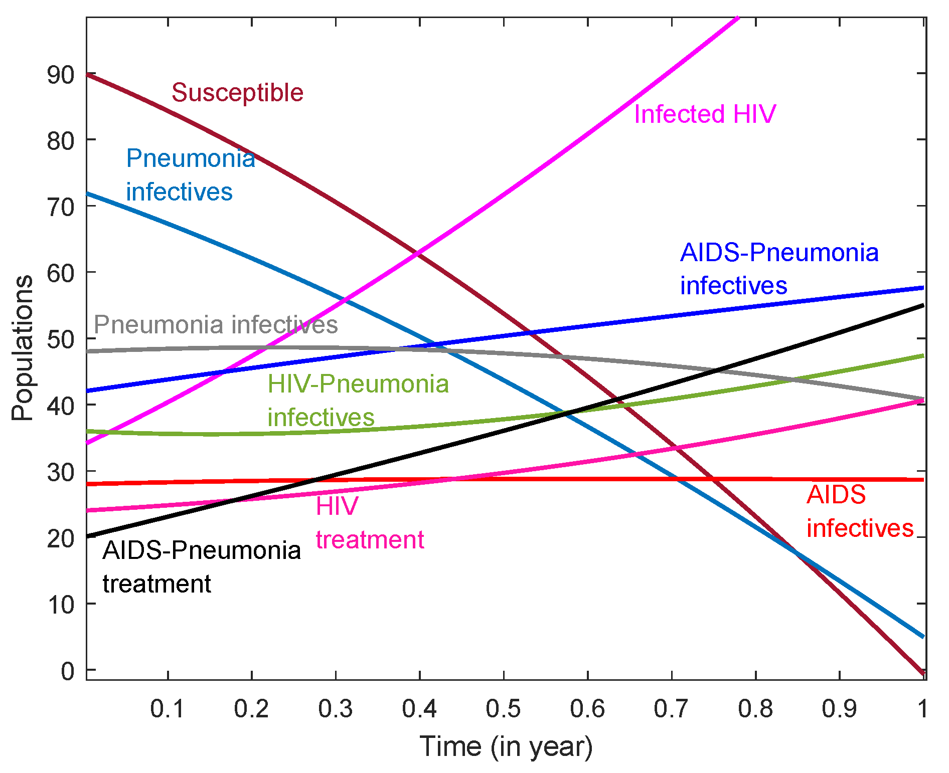
4. Numerical Simulation

Now, to verify the proposed implementation of the analytic homotopy perturbation method to find the solution of the pneumonia–HIV co-infection model, we assume the following initial values of the population classes:

$$S_0=90,I_{pn}{}_0=72,I_{HV0}=34,I_{HVpn0}=36,I_{A0}=28,I_{Apn0}=42,T_{pn0}=48,T_{HV0}=24,T_{Apn0}=20.$$

Now, by using the data from Table 1 and these initial values of the population, we obtain the following polynomials of the third degree (by using the HPM, as in the previous section; here, we calculated up to the third degree), i.e., up to three iterations:

$$S\left(t\right)=90-52.9400t-40.8500t^2+3.1400t^3,$$

$$I_{pn}\left(t\right)=72-44.6600t-25.6400t^2+3.2180t^3,$$

$$I_{HV}\left(t\right)=34+60.4500t+32.2000t^2-4.7500t^3,$$

$$I_{HVpn}\left(t\right)=36-6.3000t+21.7800t^2-4.0820t^3,$$

$$I_A\left(t\right)=28+3.1340t-3.7960t^2+1.3240t^3,$$

$$I_{Apn}\left(t\right)=42+18.2800t-3.6060t^2+0.9677t^3,$$

$$T_{pn}\left(t\right)=48+5.2800t-10.7600t^2-1.7250t^3,$$

$$T_{HV}\left(t\right)=24+7.3400t+6.8750t^2+2.4230t^3,$$

$$T_{Apn}\left(t\right)=20+30.7400t+1.1960t^2+3.0780t^3.$$

The solution obtained through the HPM was then plotted using Matlab 2020a, as shown in Figure 1. It shows the convergence of all compartments at a faster rate and gives reliable results. Figure 1 indicates the flows of various population densities in society. We observe that individuals infected with pneumonia acquire HIV, i.e., co-infection, in approximately six months, and individuals infected with HIV acquire pneumonia within just a month if precautionary measures prescribed by medical personnel are not taken within a certain amount of time. It is also observed that the population that is infected with AIDS keeps on decreasing by a small fraction. Since pneumonia is a treatable disease if its treatment is begun at right time, there is a possibility of eradicating it in an endemic situation, making it converge. In addition, we observe that the treatment of HIV infections and treatment of AIDS–pneumonia increase. This lets us conclude that, to stop the spread of co-infection, the number HIV-infected individuals should be decreased. The number of HIV-infected individuals can be reduced by creating health facilities in regions such as Africa, through medical facilities, and through earlier detection of the disease so as not allow individuals to be hosts for other opportunistic diseases, such as cytomegalovirus pneumonia.

5. Conclusions

This paper studies the co-infection dynamics of pneumonia and HIV/AIDS through the formulation of a mathematical model that comprises each individual disease and co-infections thereof, along with their treatment classes. The model comprises four equilibrium points, namely, disease-free, i.e., non-existence of either disease, the endemic equilibrium point for HIV (a society with only HIV-infected individuals), the endemic equilibrium point for pneumonia (a society with only pneumonia-infected individuals), and an endemic point at which both diseases co-exist. Therefore, formulation of the model explains the spread of pneumonia–HIV in a real society very well. The main focus of our study was to show the efficiency of the homotopy perturbation method when used to solve nonlinear differential equations. Through the numerical simulations, it was observed that solving the system with the homotopy perturbation method gave reliable results, and convergence was shown at a faster rate. The results obtained in the numerical simulations show the importance of the precautionary measures to be taken by HIV-infected individuals to keep themselves safe from co-infection with pneumonia. Hence, in comparison with pneumonia-infected individuals, HIV-infected individuals need to be more aware of their health conditions and need to take the proper medications in order to avoid other infections. However, to avoid further complications in their health conditions, individuals suffering from either disease need to take their treatments at the right time so as to prevent the spread of co-infections.

References

1. Mayilvaganan, S.; Balamuralitharan, S. Analytical solutions of influenza diseases model by HPM. AIP Conf. Proc. 2019, 2112, 020008. [Google Scholar] [CrossRef]
2. Omondi, E.O.; Mbogo, R.W.; Luboobi, L.S. Mathematical analysis of sex-structured population model of HIV infection in Kenya. Lett. Biomath. 2018, 5, 174–194. [Google Scholar] [CrossRef]
3. Khademi, F.; Yousefi-Avarvand, A.; Sahebkar, A.; Ghanbari, F.; Vaez, H. Bacterial co-infections in HIV/AIDS-positive subjects: A systematic review and meta-analysis. Folia Med. 2018, 60, 339–350. [Google Scholar] [CrossRef]
4. Lutera, J.; Mbete, D.; Wangila, S. Co-infection model of HIV/AIDS-pneumonia on the effect of treatment at initial and final stages. IOSR J. Math. 2018, 14, 56–81. [Google Scholar]
5. Huang, L.; Crothers, K. HIV-associated opportunistic pneumonias. Respirology 2009, 14, 474–485. [Google Scholar] [CrossRef] [Green Version]
6. Teklu, S.W.; Kotola, B.S. The Impact of Protection Measures and Treatment on Pneumonia Infection: A Mathematical Model Analysis supported by Numerical Simulation. bioRxiv 2022. [Google Scholar] [CrossRef]
7. Naveed, M.; Baleanu, D.; Raza, A.; Rafiq, M.; Soori, A.H.; Mohsin, M. Modeling the transmission dynamics of delayed pneumonia-like diseases with a sensitivity of parameters. Adv. Differ. Equations 2021, 2021, 1–19. [Google Scholar] [CrossRef]
8. Tilahun, G.T.; Makinde, O.D.; Malonza, D. Modelling and optimal control of pneumonia disease with cost-effective strategies. J. Biol. Dyn. 2017, 11, 400–426. [Google Scholar] [CrossRef]
9. Huo, H.F.; Chen, R. Stability of an HIV/AIDS treatment model with different stages. Discret. Dyn. Nat. Soc. 2015, 1–9. [Google Scholar] [CrossRef] [Green Version]
10. Dutta, A.; Gupta, P.K. A mathematical model for transmission dynamics of HIV/AIDS with effect of weak CD4+ T cells. Chin. J. Phys. 2018, 56, 1045–1056. [Google Scholar] [CrossRef]
11. de Carvalho, T.; Cristiano, R.; Goncalves, L.F.; Tonon, D.J. Global analysis of the dynamics of a mathematical model to intermittent HIV treatment. Nonlinear Dyn. 2020, 101, 719–739. [Google Scholar] [CrossRef]
12. Nthiiri, J.K.; Lavi, G.O.; Mayonge, A. Mathematical model of pneumonia and HIV/AIDS coinfection in the presence of protection. Int. J. Math. Anal. 2015, 9, 2069–2085. [Google Scholar] [CrossRef]
13. Onyinge, D.O.; Ongati, N.O.; Odundo, F. Mathematical model for co-infection of HIV/AIDS and pneumonia with treatment. Int. J. Sci. Eng. Appl. Sci. 2016, 2, 106–111. [Google Scholar]
14. Teklu, S.W. Mathematical analysis of the transmission dynamics of COVID-19 infection in the presence of intervention strategies. J. Biol. Dyn. 2022, 16, 640–664. [Google Scholar] [CrossRef]
15. Shen, C.; Xu, F.; Zhang, J.F. Periodic Solutions of an Infected-Age Structured HIV Model with the Latent Factor and Different Transmission Modes. Int. J. Bifurc. Chaos 2022, 32, 2250008. [Google Scholar] [CrossRef]
16. Liu, H.; Xu, F.; Zhang, J.F. Analysis of an age-structured HIV-1 Infection Model with Logistic Target cell growth. J. Biol. Syst. 2020, 28, 927–944. [Google Scholar] [CrossRef]
17. Wang, S.; Xu, F.; Rong, L. Bistability analysis of an HIV model with immune response. J. Biol. Syst. 2017, 25, 677–695. [Google Scholar] [CrossRef]
18. Biazar, J. Solution of the epidemic model by Adomian decomposition method. Appl. Math. Comput. 2006, 173, 1101–1106. [Google Scholar] [CrossRef]
19. Rafei, M.; Ganji, D.D.; Daniali, H. Solution of the epidemic model by homotopy perturbation method. Appl. Math. Comput. 2007, 187, 1056–1062. [Google Scholar] [CrossRef]
20. He, J.H. Recent development of the homotopy perturbation method. Topol. Methods Nonlinear Anal. 2008, 31, 205–209. [Google Scholar]
21. He, J.H. An elementary introduction to the homotopy perturbation method. Comput. Math. Appl. 2009, 57, 410–412. [Google Scholar] [CrossRef] [Green Version]
22. Khan, M.A.; Islam, S.; Ullah, M.; Khan, S.A.; Zaman, G.; Arif, M.; Sadiq, S.F. Application of homotopy perturbation method to vector host epidemic model with non-linear incidences. Res. J. Recent Sci. 2013, 2, 90–95. [Google Scholar]
23. Kolawole, M.; Ogunniran, M.; Alaje, A.; Kamiludeen, R.T. Simulating the Effect of Disease Transmission Coefficient on A Disease Induced Death Seirs Epidemic Model Using the Homotopy Perturbation Method. J. Appl. Comput. Sci. Math. 2022, 16, 40–43. [Google Scholar] [CrossRef]
24. Rekha, S.; Balaganesan, P.; Renuka, J. Homotopy Perturbation Method for Mathematical Modeling of Listeriosis and Anthrax Diseases. Ann. Rom. Soc. Cell Biol. 2021, 25, 9787–9809. [Google Scholar]
25. Omale, D.; Gochhait, S. Analytical solution to the mathematical models of HIV/AIDS with control in a heterogeneous population using Homotopy Perturbation Method (HPM). AMSE J. AMSE IIETA Ser. Adv. A 2018, 55, 20–34. [Google Scholar]
26. Diekmann, O.; Heesterbeek, J.A.P.; Metz, J.A. On the definition and the computation of the basic reproduction ratio R 0 in models for infectious diseases in heterogeneous populations. J. Math. Biol. 1990, 28, 365–382. [Google Scholar] [CrossRef]
27. He, J.H. Homotopy perturbation technique. Comput. Methods Appl. Mech. Eng. 1999, 178, 257–262. [Google Scholar] [CrossRef]
28. Peter, O.J.; Awoniran, A.F. Homotopy perturbation method for solving sir infectious disease model by incorporating vaccination. Pac. J. Sci. Technol. 2018, 18, 133–140. [Google Scholar]
29. Agbata, B.C.; Shior, M.M.; Olorunnishola, O.A.; Ezugorie, I.G.; Obeng-Denteh, W. Analysis of Homotopy Perturbation Method (HPM) and its Application for Solving Infectious Disease Models. Int. J. Math. Stat. Stud. 2021, 9, 27–38. [Google Scholar]
Figure 1. A plot of the different compartments used in the model that was solved by using HPM.
Foundations 02 00072 g001