Article

Survey for Soil Sensing with IOT and Traditional Systems

Department of Computer Science and Engineering, Michigan State University, East Lansing, MI 48824, USA
*
Author to whom correspondence should be addressed.
Network 2023, 3(4), 482-501; https://doi.org/10.3390/network3040021
Submission received: 8 August 2023 / Revised: 21 September 2023 / Accepted: 26 September 2023 / Published: 8 October 2023
(This article belongs to the Special Issue Innovative Mobile Computing, Communication, and Sensing Systems)

Abstract

:
Smart Agriculture has gained significant attention in recent years due to its benefits for both humans and the environment. However, the high costs associated with commercial devices have prevented some agricultural lands from reaping the advantages of technological advancements. Traditional methods, such as reflectance spectroscopy, offer reliable and repeatable solutions for soil property sensing, but the high costs and redundancy of preprocessing steps limit their on-site applications in real-world scenarios. Recently, RF-based soil sensing systems have opened a new dimension in soil property analysis using IoT-based systems. These systems are not only portable, but also significantly cheaper than traditional methods. In this paper, we carry out a comprehensive review of state-of-the-art soil property sensing, divided into four areas. First, we delve into the fundamental knowledge and studies of reflectance-spectroscopy-based soil sensing, also known as traditional methods. Secondly, we introduce some RF-based IoT soil sensing systems employing a variety of signal types. In the third segment, we introduce the details of sample pretreatment, inference methods, and evaluation metrics. Finally, after analyzing the strengths and weaknesses of the current work, we discuss potential future aspects of soil property sensing.

1. Introduction

Smart agriculture has increasingly become a focal point of interest. Implementing a smart agriculture system can assist farmers in achieving precision irrigation [1,2,3], leading to more efficient water usage. Additionally, the integration of such systems can aid farmers in monitoring their soil’s fertility levels. This not only boosts their crop yield [4], but also helps in averting over-fertilization, which can contaminate the soil and groundwater [5,6].
Soil sample measurements using reflectance spectroscopy are regarded as reliable due to their high repeatability and reproducibility [7]. These methods are also viewed as swift and cost-effective tools for soil characterization [8,9]. Traditional reflectance spectroscopy is typically conducted in laboratory settings using spectrometers [10], accompanied by several preprocessing steps. These preprocessing activities aim to minimize the effects of soil moisture and particle size, thereby reducing covariables in soil property predictions [11]. However, the preprocessing requirements further confine the experiment environment to the laboratory. A gap remains between laboratory experiments and real-world, on-site detection.
Recently, RF-based soil sensing has been introduced as a portable and cost-effective alternative for on-site soil analysis [12,13,14,15,16]. When contrasted with traditional reflectance spectroscopy experiments, RF-based techniques present several advantages. First, the equipment used, such as RFID tags of WiFi device is more widely available and affordable [12,13,14]. Second, RF-based soil sensing eliminates the need for preprocessing steps, bridging the gap between laboratory and real-world applications. Moreover, thanks to the property of RF signals, these methods can encompass a broader area compared to traditional techniques.
Given the burgeoning interest in soil property sensing, numerous studies have been undertaken to encapsulate the advancements in this domain [7,17,18,19,20,21,22]. Nevertheless, the recent advent of RF-based soil property sensing has brought to the fore IoT-based systems showcasing the potential for affordable and mobile soil sensing solutions. These emerging contributions have not been comprehensively reviewed and encapsulated. Table 1 delineates the distinctions between the topics covered in literature reviews of soil sensing methodologies over the past two decades and the content of our research.
In this study, we undertake a comprehensive review of soil property sensing methodologies, encompassing both traditional reflectance spectroscopy-based systems and RF-based IoT soil sensing systems. In addition to this, we delve into an in-depth discourse on soil sample preparation procedures and spectral information analysis methods. We also compare the merits and limitations of traditional and IoT methods, and contemplate potential directions for future soil property sensing research.
The organization of this paper is as follows: In the Section 1, we introduce the background of soil sensing. In Section 2, we present fundamental concepts related to soil reflectance spectroscopy and analyze traditional soil sensing methods based on reflectance spectroscopy, with a particular focus on key elements such as soil carbon, soil moisture, and soil macronutrients. The Section 3 outlines state-of-the-art RF-based IoT soil sensing systems. In Section 4, we detail various inference methods and evaluation metrics. In Section 5, we explore future prospects of soil property sensing, considering the strengths and weaknesses of existing approaches. Finally, we provide Section 6 to encapsulate the key points of this paper.

2. Tradicitonal Soil Sensing System

In this section, we delve into the conventional approach of soil sensing through reflectance spectroscopy. Diffuse reflectance spectroscopy [17,23] emerges as a swift, economical, and environmentally friendly method, showcasing consistent prediction outcomes when compared to previous chemical analysis. In recent times, the endeavors to harness vis-NIR-MIR reflectance spectroscopy for predicting soil attributes [17,19,20,24] are surging. Attributes such as total carbon (TC), total organic carbon (TOC), soil moisture, and essential chemical constituents like total soil nitrogen (N), extractable phosphorus (P), and potassium (K), among other foundational soil components, have garnered significant attention as researchers aim to pinpoint their absorption properties within the vis-NIR-MIR range.

2.1. Fundamentals of Soil Reflectance Spectroscopy

The utilization of reflectance spectroscopy for discerning soil characteristics has gained considerable attention, primarily due to its non-invasive nature [9,17,25]. Traditional reflectance spectroscopy is founded on the principles of the Beer–Lambert law. The Beer–Lambert law [26] explains the diminution of light intensity as it passes through a material, with this reduction being directly related to the substance’s properties. As light permeates a material, it incites the molecule bonds of each component within the substance to vibrate. Given the unique molecular structures and bonds that each chemical species possesses, each one generates a distinct absorption spectrum. Thus, the Beer–Lambert law is widely employed to determine the concentration of chemical components that can absorb and scatter light in chemical analyses [8,25,27].
One common variant of the Beer–Lambert law establishes a relationship between the decrease in light intensity within a material, which comprises a uniformly distributed absorbing substance, the length of the optical path of light through the substance, and the substance’s absorbance capacity [28,29]. The mathematical depiction of the Beer–Lambert law [30] is presented in Equation (1).
A = log ( I 0 I r ) = ϵ c
Here, I represents the light intensity that is initially emitted, while I r signifies the light intensity received after it has traversed an optical path of length . A stands for the absorbance of the substance, which can be calculated from the initial emitted light intensity I and the detected light intensity I r after the light has journeyed the optical path of length . The molar attenuation coefficient is represented by ϵ , and c denotes the concentration of the species that attenuates the light. Consequently, the frequencies where light absorption occurs result in a diminished reflected radiation signal. This can be represented in reflectance R and can subsequently be converted to apparent absorbance, as illustrated in Equation (2) [19,31].
A = log ( 1 R )

2.2. Soil Sample Pretreatment

This section details the preparation and preliminary processing of soil samples prior to spectral analysis. Regarding soil sample preparation, there are two common methodologies. Some studies involve collecting samples directly from the field [32,33,34,35], while others prefer to amalgamate raw soil with a solution that contains target elements to achieve the desired concentration levels [36]. During the pre-processing phase, multiple steps are undertaken—whether the sample is natural or mixed—to ensure the soil’s homogeneity and to mitigate interference from other sources like moisture or particle size variations.

2.2.1. Preparation of Soil Samples

The first step in soil attribute sensing is collecting soil samples. The approach to collecting soil samples can vary. Broadly, soil samples can be categorized into two groups: those collected directly from the field and those where natural soils are combined with a target element solution. In the study by [33], soil samples (0–20 cm depth) were sourced from 10 distinct rice-paddy and cropland locations in the Aceh Besar district of Aceh Province. From each location, two samples were extracted from rice-paddy fields and two from the neighboring croplands. The research in [34] utilized soil gathered from the Horticulture Research Centre in Kamrup, Assam. They employed a grid sampling method, collecting soil from 20 cm below the surface. The samples in the study by [32] came from uncultivated and unfertilized farms. Typically, such natural soil samples are also procured from about 20 cm beneath the surface.
In contrast to using only naturally collected soil, some studies aim for compatibility with higher concentration levels of the target attributes. For instance, in [36] mixed natural soils, sourced from Hui Zhuang Agricultural Development Company in Huainan City, Anhui Province, China, with Nitrogen solutions at concentrations ranging from 0% to 30% (increasing in 2% increments) for their experiments. The method of soil sample preparation is usually determined by the desired concentration levels for the target elements.

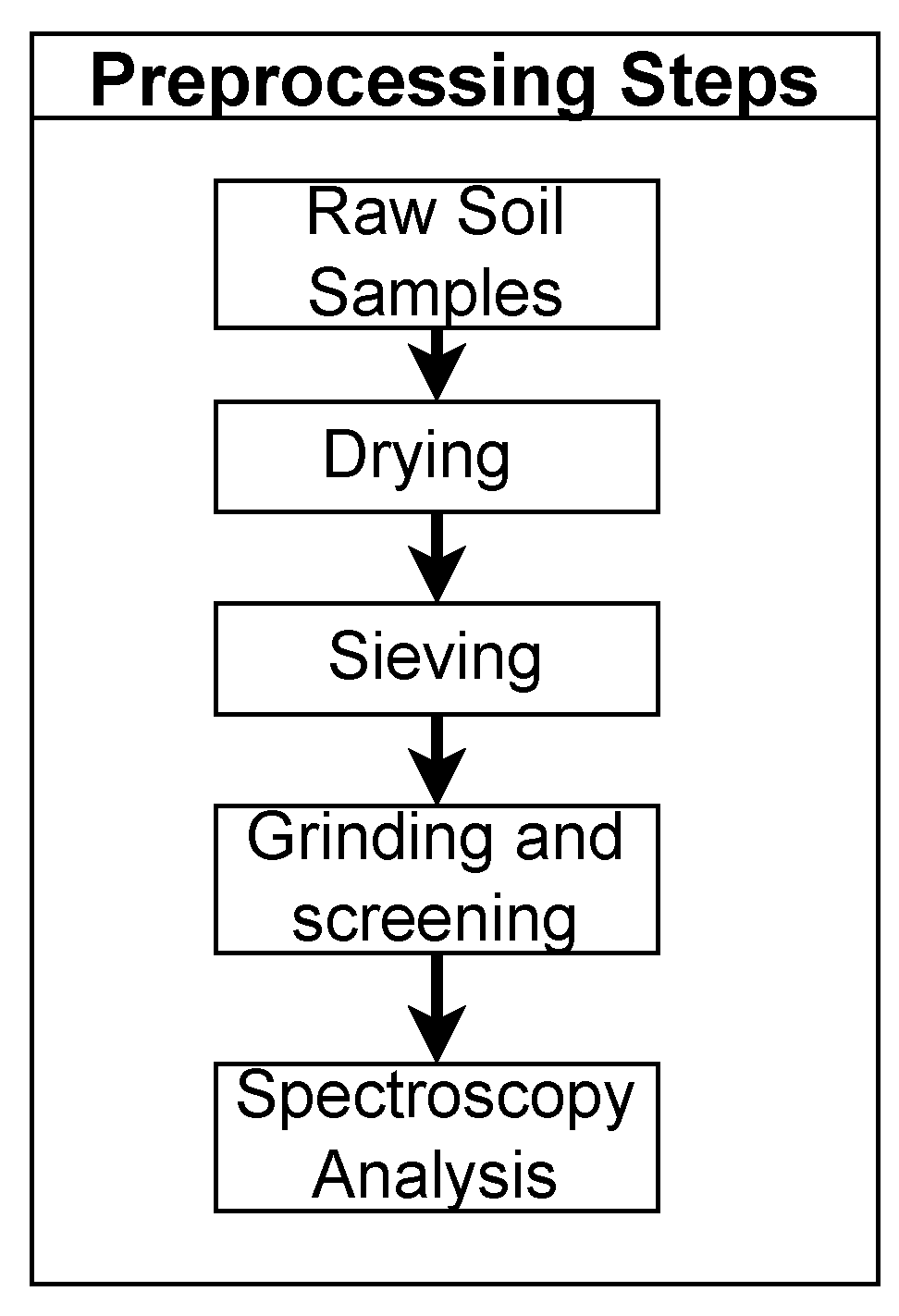
2.2.2. Pre-Processing Steps for Soil Samples

In conventional in-lab soil attribute sensing experiments, pre-processing of soil samples is a standard procedure, as evidenced by various studies [19,32,33,34,36]. Considering that spectra obtained from horizontal cross-sections of 5 cm soil slices yield slightly less precise predictions [19], such pre-processing is vital. This is because these preparatory steps ensure consistent quality across all soil samples, facilitating the development of a more generalized model based on these standardized samples.
Figure 1 depicts the procedural flow for soil sample pre-processing. The initial stage of soil pre-processing involves drying. For instance, in the study by [33], soil samples were stored for a day to equilibrate, followed by air-drying for a week. Similarly, in [34], soil samples collected from 20 cm below the soil surface were air-dried for approximately a week. In the research by [36], soil samples were dried at 80 °C for 8 h after being thoroughly mixed with varying concentration solutions. In [37], the soil samples are thinly spread, with a thickness of about 2 cm, and left to dry in a well-ventilated indoor area with ample light. After drying, the samples are transferred into beakers and further dehydrated using an electric blast dryer. The objective of dehydration is to eliminate the impact of soil moisture during the spectroscopy analysis process.
Next, sieving is the subsequent step in soil preprocessing. In the study by [33], dried soil samples are passed through a 2 mm nylon sieve to exclude stones, insects, large debris, pebbles, and other extraneous materials. Similarly, Ref. [34] filter the dried samples using a 2 mm sieve. In the research conducted by [32], hand cleaning is employed to eliminate stones and excessive residues. The primary purpose of this step is to discard materials with larger particle sizes, as they can introduce significant noise to the spectroscopy analysis.
The final preparatory step before spectroscopy analysis involves grinding and screening. In the study by [33], soil samples were ground using a mechanical agate grinder and then sieved through a 100 mesh screen (with a diameter of 0.150 mm). Similarly, in the research presented by [34], all soil samples underwent grinding. The study by [32] opted to grind their samples and subsequently sieve them through a 1 mm screen. Soil samples in [36] were first ground, then sieved using an 80 mesh (160 μ m) screen, and later compressed into 10 mm × 10 mm samples with a thickness of 2 mm under 10 MPa pressure using a bench press machine. In the study by [35], the approach involved grinding the soil samples into a powdered form and subsequently passing them through a 100-mesh sieve. The main objective of this procedure is to minimize the impact of diffuse reflectance from soil samples that are not uniformly distributed. After these steps are carried out diligently, the soil samples are prepared for in-lab spectroscopy analysis to identify the concentration levels of specific soil attributes.

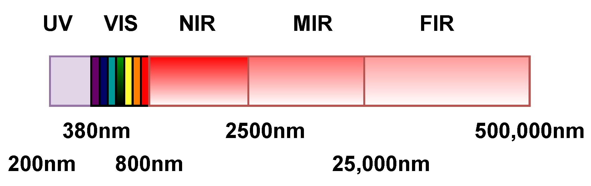
2.3. Spectral Range Selection for Reflectance Spectroscopy

For reflectance spectroscopy, multiple spectral ranges are accessible, as depicted in Figure 2. Research from [17,19] outlines the most consistently effective spectral ranges utilized in Reflectance Spectroscopy: Visible, Near-Infrared (NIR), and Mid-Infrared (MIR). Combinations of these spectra, such as Vis-NIR(VNIR) or NIR-MIR, offer potential solutions for detecting various soil properties. Spectra deemed to be either unresponsive or influenced by spectrometer artifacts were excluded before conducting the statistical analysis. The wavelength ranges for Visible, NIR, and MIR are detailed in Table 2. According to the research of [17,19,38], five spectral ranges are typically considered and employed in spectral analysis.

2.4. Total Carbon and Total Organic Carbon

An accurate evaluation of carbon content is crucial for understanding soil fertility and nutrient management. Two primary categories are studied in this domain: Total Carbon and Total Organic Carbon. TC encompasses all carbon found in every particle and compound, which includes both TOC and Total Inorganic Carbon (TIC). TC represents the entirety of carbon found in any compound or particle. Total Inorganic Carbon and Total Organic Carbon represent carbon originating from all organic sources that are covalently bound [39]. In the context of soils and sediments, the organic fraction comprises residues from animals, plants, or microorganisms at various decomposition stages, as well as elemental C like coal, charcoal, and graphite [40]. In scenarios where no inorganic carbon forms are present in soils and sediments, the quantity of TC matches the TOC value [41].
T o t a l C a r b o n = T o t a l O r g a n i c C a r b o n + T o t a l I n o r g a n i c C a r b o n
The study by [42] explored the potential of diffuse reflectance spectroscopy in predicting TC in Hawaiian agricultural soils. This was accomplished by integrating visible, NIR, and MIR spectral libraries and constructing chemometric models using partial least squares regression (PLSR) and random forest (RF) ensemble tree regression. The models achieved R 2 values of 0.95 (VNIR) and 0.94 (MIR) with RMSE values of 2.80% and 3.08%, respectively.
In a different study, Ref. [43] utilized MIR to assess organic carbon in soils using portable instruments that spanned visible-to-near-infrared and mid-infrared ranges. Their experiments, both on-site and in the laboratory, confirmed the flexibility and potential of handheld MIR instruments over stationary counterparts. The MIR models, developed from finely ground samples, achieved an impressive R 2 of 0.86 and an RMSE of 0.11% during cross-validation.
Meanwhile, Ref. [44] aimed to predict soil organic carbon using a local PLSR approach. They amassed nearly 20,000 samples from across the European Union, scanned using a VNIR spectrometer. Their results highlighted a promising predictive capability for mineral soils, with RMSE values of 3.6 g/kg for cropland and 7.2 g/kg for grassland.
An innovative calibration method, known as regression rules, was introduced by [45]. This approach offers benefits such as high accuracy, simplicity in interpretation, variable selection, parsimony, and adherence to the upper and lower prediction boundaries.
Lastly, Ref. [46] set out to calibrate and validate models for TC and TOC using approximately 20,000 samples from the Rapid Carbon Assessment Project (RaCA). This nationwide initiative gathered over 144,000 soil samples from across the U.S for carbon stock mapping using VisNIR. Models were developed using either PLSR or Artificial Neural Network (ANN). The results demonstrated that the ANN-calibrated models for OC and TC, with R 2 values exceeding 0.94, had a significant edge over the PLSR models, which had an R 2 value of 0.83. This suggests potential benefits in combining neural networks with reflectance spectroscopy.

2.5. Soil Moisture

Soil moisture is pivotal for facilitating the uptake of vital nutrients by plants. Accurate monitoring of soil moisture is key for promoting sustainable agriculture [3,47,48]. In the realm of soil moisture detection via reflectance spectroscopy, the fluctuation in light reflectance is particularly evident in the VNIR region [22,49], especially within the water absorption bands at 1450 and 1940 nm [22,50,51,52]. The findings in [50] illustrate that changes in relative reflectance based on soil moisture are contingent on moisture levels. Under typical agricultural scenarios with lower soil moisture, as moisture content rises, reflectance decreases.
However, the significance of detecting soil moisture extends beyond its own measure. It also critically impacts the detection of other soil attributes. This is because reflectance spectroscopy hinges on how incident light interacts with a material’s surface, and moisture presence can alter the absorption of other properties [53]. The research presented in [53] centers on assessing the potential of NIRS for analyzing moist field soils, gauging the influence of soil moisture on the accuracy of NIRS predictions of soil attributes, and evaluating the reliability of a NIRS multivariate calibration method. Tests on both air-dried and moist soils show that NIR-PLSR holds strong predictive accuracy for several soil attributes, including total C, organic C, inorganic C, total N, and clay.
The study [54] seeks to mitigate the moisture effect on spectra during the prediction of Soil Organic Carbon (SOC) content. It adopts the external parameter orthogonalization (EPO) technique to counteract the moisture influence on spectral calibration. Meanwhile, the research in [55] delves into SOC prediction, utilizing the normalized soil moisture index (NSMI) to determine the moisture content of samples, achieving an R 2 value of 0.74, and categorizing samples based on their spectral moisture content.
Furthermore, [56] evaluate the combined impact of salt and moisture on soil reflectance spectra. Their findings indicate that the concurrent variability of salt and moisture content complicates the modeling based on soil reflectance quantification, preventing accurate assessments of either property.

2.6. Soil Macronutrients (N, P and K)

Essential soil macronutrients, namely nitrogen, phosphorus, and potassium, are vital for plant and crop vitality [57]. Not only does accurate macronutrient detection enhance plant growth and crop yield [58], but it also mitigates risks associated with over-fertilization and groundwater contamination [59].
In [33], the researchers target the measurement of six soil properties: N, P, K, soil pH, magnesium (Mg), and calcium (Ca). Utilizing a spectrometer in the NIR region (1000–2500 nm), they gather spectral data and post certain preprocessing steps. This study also juxtaposed PCR (Principal Component Regression) and PLSR calibration methods, incorporating a PCA-based outlier detection strategy to enhance prediction model stability.
The study by [35] centers on predicting N, P, and K. When juxtaposed with [33], and [35] evaluates performance variations across diverse spectral regions, encompassing NIR, MIR, and a combination of both. Interestingly, the preprocessing in [35] omits the water removal step, which was present in [33]. This suggests that their calibration model might exhibit increased resilience to fluctuations in soil moisture levels. By employing Least Squares Support Vector Regressions (LS-SVM), they achieved superior results compared to the conventional PLSR method within the NIR or MIR spectrum. This study underscores the efficacy of LS-SVM in precisely gauging soil attributes via infrared reflectance spectroscopy.
On another front, Ref. [34] present a novel perspective on soil sensing aimed at macronutrients. Instead of traditional spectrometers, they employ LEDs and sensors embedded on a circuit board. However, there are certain limitations to their approach. For one, even when taking into account the LEDs’ lower resolution compared to traditional spectrometers, the target element concentration level span (0 to 50%) seems considerably elevated relative to prior research. Additionally, instead of leveraging conventional calibration models such as PLSR, LS-SVR, or neural networks, Ref. [34] utilize a unique curve for their predictive model. This approach might constrain the model’s generalizability. Notwithstanding these concerns, their research ushers in an innovative perspective on reflectance spectroscopy by harnessing LEDs and sensors, marking significant progress towards real-world, on-location deployments versus controlled lab-based experiments with spectrometers.
The study by [60] showed that, without the presence of coarse crumb, PLSR could accurately determine soil attributes such as Total Nitrogen (TN), Total Phosphorus (TP), and Total Potassium (TK) in a laboratory setting using vis-NIR reflectance spectra. This research provided a rapid technique for soil classification aligned with the Chinese Soil Taxonomy (CST) by tapping into properties linked to CST.
Regarding individual macronutrient detection, Ref. [61] formulated a hyperspectral model, emphasizing Soil Nitrogen (SN) estimation, grounded on the PLSR calibration method. Samples were sourced from diverse agricultural lands in Maharashtra, India, enhancing the model’s versatility. The research identified several spectral bands sensitive to soil nitrogen content, including 480 nm, 511 nm, 653 nm, 997 nm, 1472 nm, 1795 nm, 2210 nm, and 2296 nm.
Certain studies deeply analyze nitrogen detection, intertwining this process with other crucial elements like TC [62]. Specifically, Ref. [62] crafted a methodology for swift on-site evaluations of C and N using a portable spectroradiometer, the ASD FieldSpecPro. The study highlighted that the accuracy of PLSR-based calibration improves when the training datasets align spectrally with the target datasets. In related work, Ref. [63] indicated that training and testing phosphorus detection on soil samples from diverse fields amplifies the complexity, making practical applications more challenging. The research by [64] underscored that the prediction of total phosphorus is linked to SC detection in the NIR spectrum. Moreover, Ref. [65] embarked on detecting soil phosphorus and potassium using a vast dataset comprising over 1500 soil samples. Opting for the 1100 to 2500 nm range within the VNIR spectral region, they aimed for reliable prediction outcomes. However, they observed that the optical estimation for accessible soil P and K might display inconsistencies, given its dependence on the covariation of nutrient concentrations with other soil properties, rendering prediction outcomes susceptible to perturbations.
Gleaning insights from the aforementioned studies, it is evident that the precision of soil macronutrient detection oscillates based on the choice of training and testing data derived from soil samples. Incorporating a broader spectrum of soil samples bolsters the calibration model, especially when confronting unfamiliar soil types. Furthermore, there is a discernible correlation between macronutrients, particularly N and P, and SC content [62,66]. This highlights a prospective avenue to segregate macronutrient detection from SC metrics. A noticeable trajectory in macronutrient detection methods also emerges, shifting from laboratory-based spectrometers [33,35] to field-compatible Printed Circuit Boards (PCB), underscoring the potential for on-the-ground, cost-effective, real-time macronutrient detection systems.
Table 3 provides a summary of traditional methods used for detecting soil TC, TOC, soil moisture, and soil macronutrients. The table reveals two notable trends in traditional soil sensing research. Firstly, calibration techniques have evolved from PCR to PLSR, and now LS-SVM and ANN are gaining prominence due to advancements in computational methods and neural networks. Secondly, there is a growing emphasis on the VNIR spectral range, as these wavelengths are more readily available and offer promising applications for field deployments.
However, it is important to note that simply relying on the R 2 value is not sufficient for assessing the efficacy of these systems, as some studies do not provide the scale or range of concentration levels. A higher concentration range is more likely to result in a higher R 2 value. Additionally, all these studies involve preprocessing steps that, while improving generalizability and system stability, also hinder their direct application in real-world settings.

3. RF-Based Soil Sensing Systems in Internet of Things (IoT)

In recent times, the convergence of soil property sensing and the Internet of Things (IoT) has garnered increasing interest. While the advent of IoT in soil sensing has been relatively recent, its potential impact on advancing smart agriculture has been profound. A pivotal application of this is intelligent irrigation, which not only enhances plant growth and quality, but also conserves water resources [67]. Current soil moisture sensors are often prohibitively expensive for individual pot deployment [68]. The essence of RF-based IoT soil sensing revolves around remotely monitoring soil moisture levels. This technological shift encompasses a range of RF signals, from Wi-Fi and RFID to LTE and LoRa.
Compared to traditional soil sensing methods, which rely on intricate chemical spectral analysis and often entail elaborate preprocessing steps [32,33,35,36,37,69] or specialized equipment like spectrometers [33,35,36,37,63], the benefits of IoT in soil sensing are clear-cut. Firstly, the investment required for IoT systems is generally lower than that for commercial devices [68]. Modern IoT-based soil moisture sensors are cost-effective. While commercial alternatives often exceed $ 100 , these systems are typically priced below that threshold, yet they deliver performance on par with premium devices. Secondly, the adaptability of IoT systems is commendable; they can be seamlessly integrated beneath the soil’s surface [12,13,15,16].
Lastly, these systems are equipped with extensive communication capabilities and compatible with several types of soil surfaces as shown in Figure 3. For instance, the system in [16] boasts a communication range of 100 ms, while [15] extends this to an impressive 2.4 km.

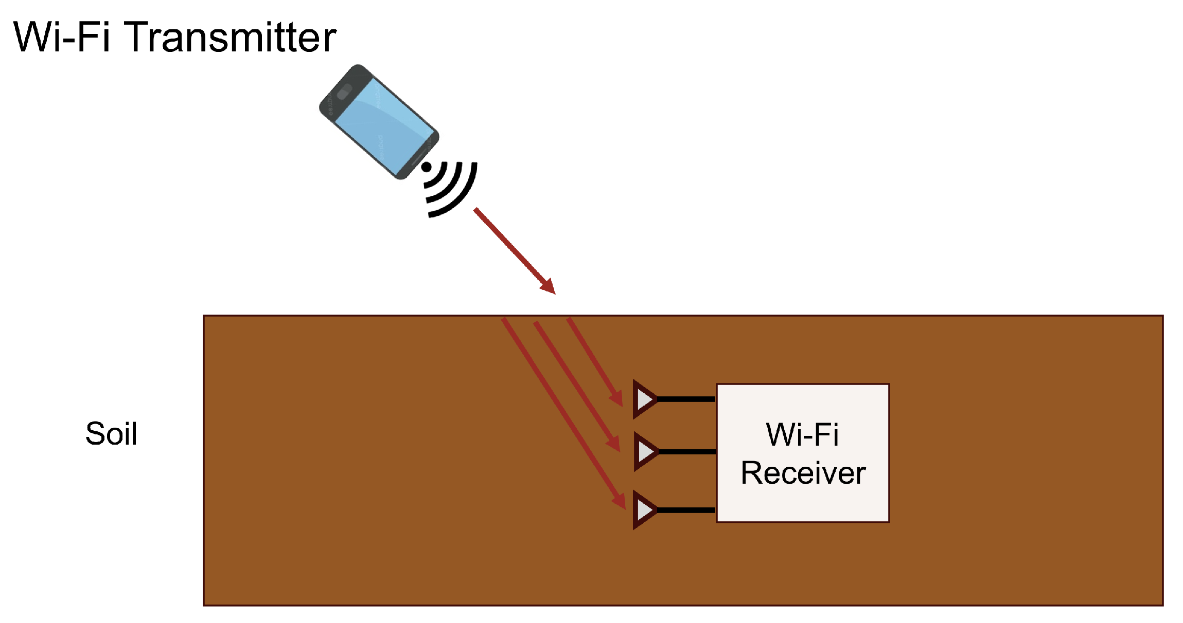
3.1. Wi-Fi Based Soil Sensing Systems

In the study by [12], Wi-Fi technology is incorporated into the realm of smart agricultural soil sensing to measure soil moisture and electrical conductivity (EC). Their system, which is called Strobe, is devised to detect soil moisture and EC by leveraging RF propagation within prevalent Wi-Fi bands. The system overview of Strobe is shown in Figure 4.
Strobe correlates the Wi-Fi time of flight (ToF) across several antennas and the amplitude ratios of these signals to the soil permittivity and EC, attributes influenced by the soil’s moisture and salinity levels. The equation showcases the correlation between the RF signal’s propagation speed and the soil moisture level, as depicted in Equation (4) [12]. Using the speed of light and the Time of Flight (ToF) τ over a specified distance d with the speed of light c, the apparent permittivity ϵ w i f i can be determined.
ϵ w i f i = ( c τ d ) 2
Their research effectively highlights the benefits of IoT devices, which are considerably more affordable than traditional commercial devices that can cost upwards of thousands of dollars.
Another study [13] adopts the center frequency of 2.5 GHz for the soil moisture sensing task. They introduce CoMEt, an RF-based technique that gauges soil moisture across multiple depths beneath the ground surface without embedding any equipment into the soil or directly contacting the ground. CoMEt’s primary insight is the dependency of an RF signal’s phase on its wavelength in the transmitting medium, which in turn is influenced by soil moisture levels. They establish a correlation between the wavelength and the apparent dielectric permittivity, ϵ , which allows CoMEt to compute ϵ using the deduced wavelength values l, as illustrated in Equation (5) [13].
ϵ = ( c f l ) 2
Subsequently, they employ the Topp Equation [70] to link the soil’s volumetric water content (VWC) ϕ with the apparent dielectric permittivity, as represented in Equation (6) [70]. CoMEt can estimate the moisture content in each layer of the soil.
ϕ = 4.3 × 10 6 ϵ 3 5.5 × 10 4 ϵ 2 + 2.92 × 10 2 ϵ 5.3 × 10 2
The system is implemented with a software-defined radio paired with a Raspberry Pi, allowing real-time soil moisture measurement. In evaluations conducted in indoor and outdoor settings, CoMEt determined soil moisture across three soil layers with a median error of merely 1.1%.

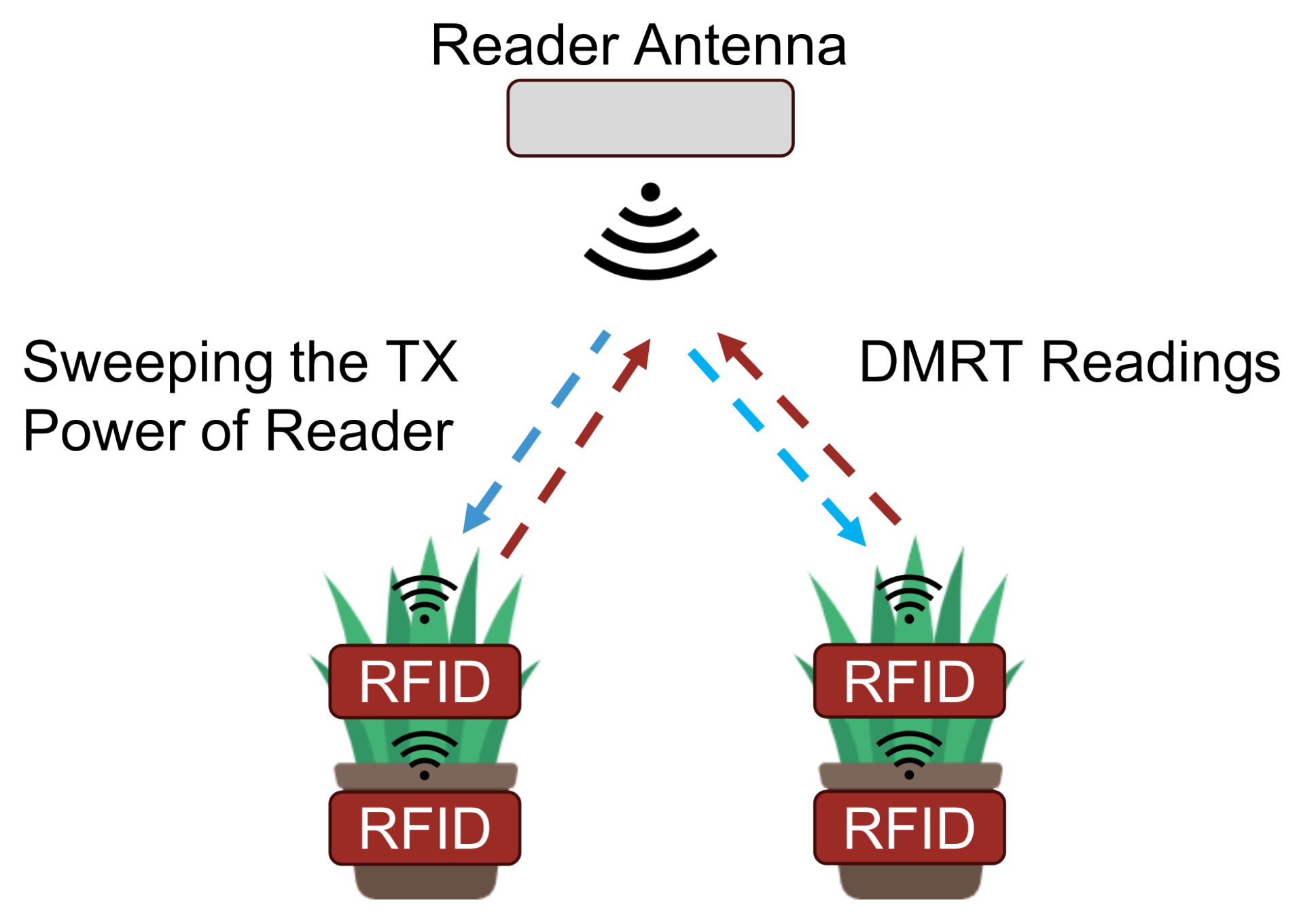
3.2. RFID-Based Soil Sensing Systems

In their research, Ref. [14] presents GreenTag, an economical RFID-based system for soil moisture detection. They utilize two RFID tags attached to a plant container to convert soil moisture content variations into their Differential Minimum Response Threshold (DMRT) metric at the reader. Commercial RFID readers offer three signal metrics: Minimum Response Threshold ( M R T ), Received Signal Strength ( R S S ), and phase. These can be broken down into components influenced by the soil moisture level, as detailed in Equations (7)–(9) [14]. The constants C m , C r , and C p play specific roles; C m represents the tag’s receiving sensitivity. C r and C p pertain to the amplitude and phase of both the reader’s transmitted signal and the reflection coefficient of the tag’s chip. Parameters h a and h T characterize the channels over the air and the tag’s antenna, respectively, while theta encapsulates phase information over the air and tag via θ a and θ t .
M R T = C m 20 log | h a | 20 log | h T |
R S S = C r + 40 log | h a | + 40 log | h T |
P h a s e = C p + 2 θ a + 2 θ T
The system design of GreenTag is shown in Figure 5.
With the incorporation of a low-pass filter to the DMRT metric, their approach effectively compensates for fluctuations in the external RF environment due to factors like human movements and changes in pot positioning or pot orientation. Impressively, GreenTag boasts a 90th percentile moisture estimation error of just 5%, aligning closely with the 4% errors of high-end soil moisture sensors. The system’s efficacy was tested in an actual greenhouse setting. Given its affordability and precision comparable to premium soil moisture sensors, GreenTag holds significant promise in enhancing greenhouse productivity and revolutionizing smart greenhouse irrigation techniques.

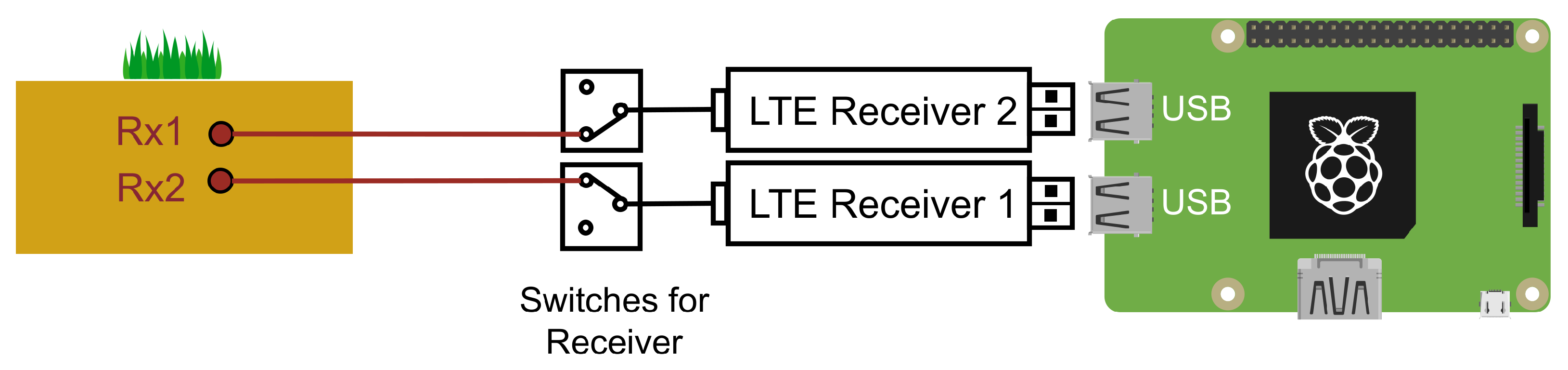
3.3. LTE-Based Soil Sensing Systems

The prior studies by [12,14] introduced RF-based methods for soil moisture sensing. While these approaches emphasize affordability, Ref. [15] focuses on reducing additional device requirements and enhancing energy efficiency. The systems presented in the earlier works necessitate power for the signal emitters (such as Wi-Fi or RFID readers) or both transceivers (like Wi-Fi AP and clients), which may hinder their large-scale outdoor deployment. In contrast, the research in [15] presents an economical LTE-based soil moisture sensor using readily available commercial hardware. Unlike Wi-Fi or RFID systems, the LTE-based setup does not require any additional hardware for signal transmission, capitalizing on the widespread presence of base stations. Figure 6 shows the hardware arrangement of their system on the LTE-receiving stage.
Central to their method is the linkage they draw between the phase changes of the intercepted LTE signal, soil moisture, and dielectric permittivity. Initially, they utilize an empirical equation to delineate the connection between the dielectric constant ϵ and volumetric water content (VWC) M o i , as presented in Equation (10) and as per [70].
M o i = 0.1138 ϵ 0.1758 .
Through the measurement of the RF wave propagation speed c s in the intended soil, the dielectric constant can be deduced with the light speed in the air c o as illustrated in Equation (11) [15].
ϵ = c 0 c s .
Hence, the soil moisture M o i can be inferred from the propagation speed c s of the RF signal within the target soil. The propagation speed of the RF signal can be deduced from the spacing between two receiving antennas d and the refraction angle θ . Additionally, γ represents the time difference of signal arrival between the two antennas, as expressed in Equation (12).
c s = d sin θ γ
They also introduce an auto-calibration mechanism for phase offset, addressing hardware limitations and minimizing the sensor’s energy consumption. Their energy-efficient design allows the system to operate on battery power for up to 16 months. Not only is their system considerably more affordable ($55) compared to traditional devices ($850), but it also boasts a remarkable accuracy (3.15%), rivaling that of premium soil moisture sensors through extensive experiments. This research significantly advances the application of RF sensing in real-world smart agriculture scenarios.

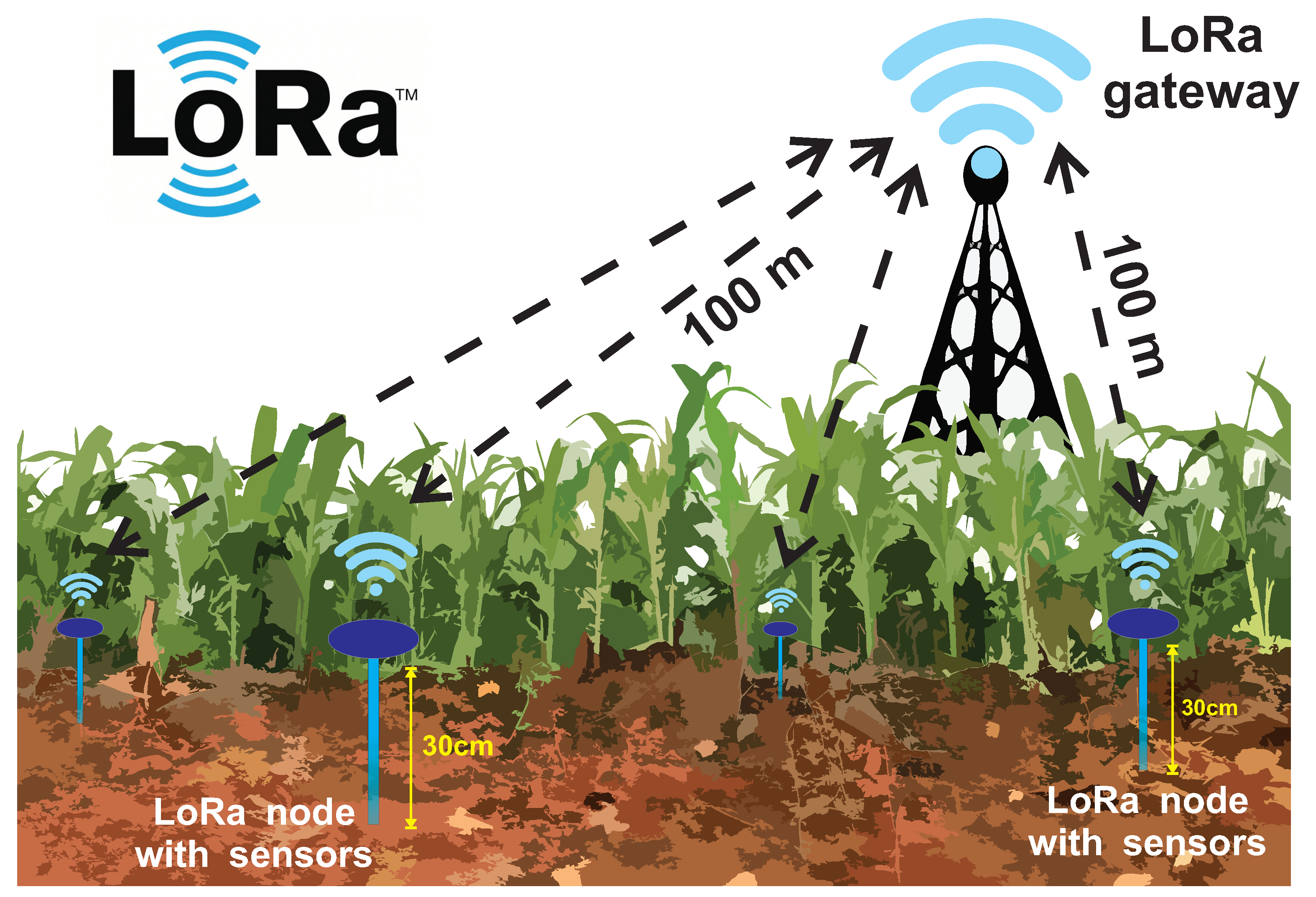
3.4. LoRa-Based Soil Sensing Systems

The work of [16] is the first practical deployment of soil moisture measurement using LoRa signals in open environments. In their study, the authors introduce a system that utilizes LoRa signals to measure soil moisture without the need for specialized sensors embedded in the soil. An overview of their system is depicted in Figure 7. The antennas of the LoRa nodes are embedded in the soil. The LoRa nodes act as transmitters, whereas the LoRa gateway functions as a receiver, capable of connecting to multiple LoRa nodes. In contrast to signal types such as RFID or Wi-Fi, the LoRa gateway, which functions as a receiver, boasts greater capacity owing to its employment of modulated chip signals. This results in reduced interference among numerous concurrently transmitted LoRa chirp signals, each utilizing distinct wavelengths, bandwidths, or chip slopes. Conversely, signal categories like Wi-Fi exhibit heightened contention among concurrently transmitted signals at the receiving terminal.
Their novel approach extends beyond merely using LoRa for data transmission in smart agriculture; they incorporate a cost-effective RF switch to alter the signal propagation path length, enabling precise moisture sensing. The soil moisture can be accurately determined with the transmission of a single LoRa packet from the node to the gateway. The underlying principle is that the soil’s dielectric permittivity, which is closely linked to its moisture level, can be derived from the phase readings of LoRa signals, as outlined in Equations (5) and (6) in the work of [13]. To tackle the synchronization challenges between the LoRa transmitter and receiver, they introduce a cost-effective switch that outfits the LoRa node with dual antennas. Experimental results with standard LoRa nodes indicate that their system can reliably gauge soil moisture with an average error of just 3.1%, matching the performance of premium soil moisture sensors. Field evaluations confirm the system’s capability to accurately detect soil moisture from a distance of 100 m between the LoRa gateway and node. Moreover, the system demonstrates resilience to interruptions from pedestrians and moving vehicles, highlighting its robust performance in outdoor environments.
Table 4 provides a comparative summary of various IoT-based soil sensing technologies, evaluating them on metrics such as Cost, Coverage Range, Central Frequency, Energy Consumption, Node Capacity, and Prediction Error. The table reveals that soil moisture sensing systems utilizing LoRa or LTE technologies tend to offer a larger coverage range. Additionally, solutions based on LoRa or RFID excel in terms of energy efficiency and sensor node capacity. These systems are also relatively cost-effective compared to traditional soil reflectance spectroscopy, making them promising candidates for deployment in remote areas without the need for pre-processing steps. The future direction for these enhanced systems involves expanding their capability to detect a broader range of soil attributes.

4. Inference Method and Evaluation Metrics

In this section, we will discuss several inferential methods and widely used evaluation metrics used in soil property sensing systems. Section 4.1 introduces the prevalent methods of spectral analysis used for inference. And Section 4.2 deals with common evaluation metrics frequently used in most studies.

4.1. Method for Spectral Information Analysis

In the analysis phase for multivariate spectral data collected from spectrometers, several methods are frequently employed to construct regression models. These models aim to predict the concentration level of target elements based on input data (predictors). Initially, we will delve into two prominent linear regression techniques: Principal Component Regression [71] and Partial Least Square Regression [72,73,74]. Following these, we will discuss the Uninformative Variable Elimination (UVE) method that is grounded on PLSR [36,75,76]. Subsequently, we will introduce the machine learning-inspired method, Least Squares Support Vector Regressions, offering an alternative perspective on spectral data analysis.

4.1.1. Principal Component Regression

Principal Component Regression is a foundational regression technique employed to establish a relationship between independent (predictor) and dependent (response) variables in a linear regression framework [71]. PCR leverages Principal Component Analysis and uses the primary components, notably those with significant variances, as the predictors in place of the original data points for regression [71,77]. In the study by [33], a comparison was made between the PCR model performance and the PLSR method. Typically, the PLSR approach requires fewer latent variables than PCR for comparable model outcomes.

4.1.2. Partial Least Square Regression

Partial Least Square Regression is a modeling method commonly used in chemometrics for spectroscopy analysis [72,73,74]. It is used to build a predictive linear regression model with independent variables X (predictor) and dependent variables Y (responses). In this paper, the independent variable X comprises the original spectrum information collected from the photodiode, exhibiting high collinearity within each channel. The concentration level of a target macronutrient (e.g., nitrogen) serves as the dependent variable Y that needs to be predicted using the independent variables X and the PLS regression model. During the analysis process, both X and Y are decomposed into multiple principal components (PC) to form a linear combination of the original data, which is then projected onto a new space using latent variables [73,74]. This process can be represented by Equations (13) and (14) [74].
X = T P T + E
Y = U Q T + F
The predictor X is represented by an n × m matrix, where n denotes the number of samples, and m corresponds to the number of available spectra. The response Y is an n × p matrix, with p indicating the number of prediction targets. For example, p = 1 to investigate the relationship between the spectral matrix X and the responses Y associated with a single target, such as the concentration level of nitrogen. The error terms from each projection equation are denoted as E and F. The score matrices of X and Y are represented by T and U, respectively, both having dimensions of n × l . The loading matrices for X and Y are denoted as P and Q, with dimensions of m × l and p × l , respectively. Here, l represents the selected number of principal components, which convert the predictor X (spectral matrix) and the response Y into linear combinations of latent variables [73,74]. The choice of principal components directly influences the precision and stability of the model. If the number of principal components is too small, some channels’ spectral information will be restricted. Conversely, selecting too many principal components introduces additional noise that may affect the system’s predictions. Therefore, selecting principal components aims to capture as much spectral information as possible while minimizing the impact of noise by choosing an appropriate number of latent variables. In the study by [32], the authors utilized the PLSR model on data obtained from LED reflection to estimate the concentration of nitrogen. They achieved a coefficient of determination ( R 2 ) of 0.875 for the calibration set and 0.803 for the validation set.

4.1.3. Uninformative Variable Elimination Method

In spectral analysis of soil properties sensing, high spectral resolution spectrometers are utilized, producing a vast number of wavelength variables suitable for the PLSR method. However, not all wavelengths contribute equally to predicting the desired element. Some are either insensitive to the target property or are susceptible to noise. The Uninformative Variable Elimination Method is employed to identify the most pertinent set of wavelengths by evaluating the cross-validation metrics of resulting models [36,75,76]. Building on the UVE method, the study by [78] introduced a Monte Carlo (MC) strategy [79] to UVE-PLS, replacing the leave-one-out approach. This novel method, named the ensemble of Monte Carlo uninformative variable elimination (EMC-UVE), refines wavelength selection during data analysis and enhances prediction capabilities for multivariate calibration models. However, the study by [36] found that while UVE can discard irrelevant wavelengths, it might also inadvertently remove valuable ones. Therefore, determining the correct number of wavelengths to retain is crucial.

4.1.4. Least Squares Support Vector Regressions

Support Vector Machines is a supervised learning method commonly used for classification tasks, such as pattern recognition [80], and regression tasks, such as data analysis and result prediction [81,82]. SVM operates based on statistical theory and maps input data to a higher-dimensional feature space [82]. However, the high computational burden associated with SVM limits its applicability in certain scenarios. To address this, the LS-SVR was introduced for regression tasks. LS-SVR simplifies the quadratic programming problem of SVM into a linear system, which can be efficiently solved using iterative methods [83]. The LS-SVR model for function estimation can be expressed as shown in Equation (15) [83].
f ( x ) = i = 1 N α i K ( x , x i ) + b
X represents the input of spectral information collected by the photodiode and f ( x ) is the target concentration level of macronutrient. The Lagrange multipliers, denoted as α i , represent the support values, while the bias term is denoted as b. The kernel function K ( x , x i ) plays a crucial role in SVM, and there are various options for kernel selection, such as the linear kernel, polynomial kernel, and radial basis function kernel (RBF kernel).
The equations for these three kernels are shown in Equations (16)–(18) [83]
K ( x , x i ) = x , x i
K ( x , x i ) = ( x , x i + p ) d
K ( x , x i ) = exp ( x x i 2 2 σ 2 )
· , · denotes the dot product, p is the bias term, and d is the index for the polynomial kernel, σ 2 is the bandwidth of RBF kernel. Using Grid Search [84] to optimize the parameters of LS-SVR not only ensures prediction accuracy, but also significantly reduces training time. However, in the study by [36], the application of a nonlinear support vector machine method did not yield particularly favorable results in terms of the Root-Mean-Square-Error (RMSE) on the cross-validation set when compared to the performance of PLSR.

4.2. Evaluation Metrics

To assess the performance of models predicting the target element, two prevalent metrics are typically used to gauge the relationship between predicted values and the actual ground truth (dependent variable): the Correlation Coefficient (R) and the Coefficient of Determination ( R 2 ). The equations for R and R 2 are provided in Equations (19) and (20), respectively [85].
r = k = 1 m ( y k y ¯ ) ( y k y ¯ ) k = 1 m ( y k y ¯ ) 2 k = 1 m ( y k y ¯ ) 2
R 2 = 1 k = 1 m ( y k y k ) 2 k = 1 m ( y k y ¯ ) 2
where y k is the predicted value of kth sample and y k is the ground truth of the kth sample. m is the total number of experiment samples. y ¯ and y ¯ is the mean value of the ground truth and prediction. The correlation coefficient r ranges between −1 and 1. The coefficient of determination R 2 = 1 if the predicted value y k exactly matches the observed value y k . A negative value of R 2 suggests that the chosen model performs poorer than a simplistic model that merely predicts the mean of the observed values.
Three vital metrics used to evaluate model performance are the root mean square error of calibration ( R M S E C ), root mean square error of prediction ( R M S E P ), and root mean square error of cross-validation ( R M S E C V ). These indicators measure the prediction errors of the model on the different data groups applied to the model. The formulas to compute R M S E C , R M S E P , and R M S E C V are given below [86]:
R M S E C = l = 1 L c ( y l ^ y c l ) 2 L c
R M S E P = l = 1 L p ( y l ^ y p l ) 2 L p
R M S E C V = l = 1 L c v ( y l ^ y c v l ) 2 L c v
where l is the sample number, L c , L p , and L c v are the total number of samples in the calibration, validation, and prediction groups. y c l , y p l , and y c v l are the predicted concentration values of the target element from the validation group and prediction group. The selection of evaluation metrics can vary between studies based on factors such as sample size and specific research objectives. For instance, R M S E C V is versatile and can be applied irrespective of the total sample count, whereas R M S E P is typically favored for studies with a larger dataset. As demonstrated in [33], they employed a combination of R M S E C and R M S E C V for assessment. Conversely, [32] relied on R M S E C and R M S E P . [35] adapts R M S E P and R M S E C V during the evaluation. A comprehensive evaluation was observed in [36], where all three metrics were utilized, providing a well-rounded assessment of their system’s stability.

5. Future Aspect

In terms of hardware, while spectrometers offer an exact resolution for spectral data, their high cost (exceeding $15k) and stringent environmental requirements significantly limit their applicability in field studies for soil reflectance spectroscopy. Meanwhile, the rise of RF-based soil sensing technology presents an enticing potential for soil property sensing due to its low-cost equipment and wide coverage area. Many of these RF systems can also remain operational for long periods when deployed in the soil. However, currently, RF-based soil sensing primarily detects soil moisture levels only. As a result, a Printed Circuit Board (PCB)-based soil sensing system could be an optimal solution in the future, striking a balance between device cost and sensing capabilities. From a preprocessing perspective, it is essential to simplify these steps to transition from laboratory-based experiments to real-world applications. To accomplish this, we need to address the influences of particle size and soil moisture levels on reflectance spectroscopy and ensure the stability of prediction models for targeted soil attributes. On the computational methods front, Partial Least Square Regression (PLSR) is widely acknowledged as the go-to calibration technique used in spectral data analysis. However, Least Square-Support Vector Regression (LS-SVR) also presents acceptable, and at times superior, prediction results compared to PLSR. Further advancements in neural network methodologies will undoubtedly benefit these computational approaches.

6. Conclusions

In this research, we present an overview of methods for sensing soil properties, covering both conventional systems based on reflectance spectroscopy and emerging IoT systems utilizing RF technologies. The study elaborates on foundational principles and preprocessing requirements in soil reflectance spectroscopy, focusing on key areas such as soil carbon content, organic carbon, moisture, and macronutrients. The paper also highlights cutting-edge IoT-based RF systems for soil analysis. To facilitate comparison, we include two summary tables that contrast results from both traditional and IoT-based approaches. Additionally, we delve into various methods for data interpretation and the metrics used for evaluating the outcomes of soil spectral assessments. In the concluding section, we examine potential future directions in the field of soil property sensing. Overall, this paper serves as an all-inclusive guide to soil property sensing, encompassing methods of sensing, preprocessing, property identification, data interpretation, and evaluation.

Author Contributions

Conceptualization, T.L. and J.W.; Methodology, J.W.; Software, J.W.; Validation, X.Z. and J.W.; Formal analysis, J.W. and T.L.; Investigation, X.Z. and L.X.; Resources, T.L. and J.W.; Data curation, J.W., T.L., X.Z. and L.X.; Writing—original draft preparation, J.W. and X.Z.; Writing—review and editing, T.L. and L.X.; Visualization, J.W. and X.Z.; Supervision, T.L. and L.X.; Project administration, T.L. and L.X. All authors have read and agreed to the published version of the manuscript.

Funding

This research received no external funding.

Data Availability Statement

No new data were created or analyzed in this study. Data sharing is not applicable to this article.

Conflicts of Interest

The authors declare no conflict of interest.

References

  1. Adeyemi, O.; Grove, I.; Peets, S.; Norton, T. Advanced monitoring and management systems for improving sustainability in precision irrigation. Sustainability 2017, 9, 353. [Google Scholar] [CrossRef]
  2. Lipper, L.; Thornton, P.; Campbell, B.M.; Baedeker, T.; Braimoh, A.; Bwalya, M.; Caron, P.; Cattaneo, A.; Garrity, D.; Henry, K.; et al. Climate-smart agriculture for food security. Nat. Clim. Chang. 2014, 4, 1068–1072. [Google Scholar] [CrossRef]
  3. García, L.; Parra, L.; Jimenez, J.M.; Parra, M.; Lloret, J.; Mauri, P.V.; Lorenz, P. Deployment strategies of soil monitoring WSN for precision agriculture irrigation scheduling in rural areas. Sensors 2021, 21, 1693. [Google Scholar] [CrossRef]
  4. Halvorson, A.D.; Nielsen, D.C.; Reule, C.A. Nitrogen fertilization and rotation effects on no-till dryland wheat production. Agron. J. 2004, 96, 1196–1201. [Google Scholar] [CrossRef]
  5. Weinbaum, S.A.; Johnson, R.S.; DeJong, T.M. Causes and consequences of overfertilization in orchards. HortTechnology 1992, 2, 112b–121. [Google Scholar] [CrossRef]
  6. Wu, Y.; Chen, J.; Wu, X.; Tian, Q.; Ji, J.; Qin, Z. Possibilities of reflectance spectroscopy for the assessment of contaminant elements in suburban soils. Appl. Geochem. 2005, 20, 1051–1059. [Google Scholar] [CrossRef]
  7. Viscarra Rossel, R.A.; Behrens, T.; Ben-Dor, E.; Chabrillat, S.; Demattê, J.A.M.; Ge, Y.; Gomez, C.; Guerrero, C.; Peng, Y.; Ramirez-Lopez, L.; et al. Diffuse reflectance spectroscopy for estimating soil properties: A technology for the 21st century. Eur. J. Soil Sci. 2022, 73, e13271. [Google Scholar]
  8. Brown, D.J.; Shepherd, K.D.; Walsh, M.G.; Mays, M.D.; Reinsch, T.G. Global soil characterization with VNIR diffuse reflectance spectroscopy. Geoderma 2006, 132, 273–290. [Google Scholar] [CrossRef]
  9. Christy, C.D. Real-time measurement of soil attributes using on-the-go near infrared reflectance spectroscopy. Comput. Electron. Agric. 2008, 61, 10–19. [Google Scholar] [CrossRef]
  10. Spectrometer. Available online: https://bimedis.com/a-item/spectroscopy-equipment-bfrl-wqf-510-1946874 (accessed on 8 August 2023).
  11. Dotto, A.C.; Dalmolin, R.S.D.; Grunwald, S.; ten Caten, A.; Pereira Filho, W. Two preprocessing techniques to reduce model covariables in soil property predictions by Vis-NIR spectroscopy. Soil Tillage Res. 2017, 172, 59–68. [Google Scholar]
  12. Ding, J.; Chandra, R. Towards low cost soil sensing using Wi-Fi. In Proceedings of the 25th Annual International Conference on Mobile Computing and Networking, Los Cabos, Mexico, 21–25 October 2019; pp. 1–16. [Google Scholar]
  13. Khan, U.M.; Shahzad, M. Estimating soil moisture using RF signals. In Proceedings of the 28th Annual International Conference on Mobile Computing and Networking, Sydney, Australia, 17–21 October 2022; pp. 242–254. [Google Scholar]
  14. Wang, J.; Chang, L.; Aggarwal, S.; Abari, O.; Keshav, S. Soil moisture sensing with commodity RFID systems. In Proceedings of the 18th International Conference on Mobile Systems, Applications, and Services, Toronto, ON, Canada, 15–19 June 2020; pp. 273–285. [Google Scholar]
  15. Feng, Y.; Xie, Y.; Ganesan, D.; Xiong, J. LTE-Based Low-Cost and Low-Power Soil Moisture Sensing. In Proceedings of the 20th ACM Conference on Embedded Networked Sensor Systems, Boston, MA, USA, 6–9 November 2022; pp. 421–434. [Google Scholar]
  16. Chang, Z.; Zhang, F.; Xiong, J.; Ma, J.; Jin, B.; Zhang, D. Sensor-free soil moisture sensing using lora signals. In Proceedings of the ACM on Interactive, Mobile, Wearable and Ubiquitous Technologies, Atlanta, USA and Cambridge, UK, 11–15 September 2022; Volume 6, pp. 1–27. [Google Scholar]
  17. Rossel, R.V.; Walvoort, D.; McBratney, A.; Janik, L.J.; Skjemstad, J. Visible, near infrared, mid infrared or combined diffuse reflectance spectroscopy for simultaneous assessment of various soil properties. Geoderma 2006, 131, 59–75. [Google Scholar] [CrossRef]
  18. Nduwamungu, C.; Ziadi, N.; Parent, L.É.; Tremblay, G.F.; Thuriès, L. Opportunities for, and limitations of, near infrared reflectance spectroscopy applications in soil analysis: A review. Can. J. Soil Sci. 2009, 89, 531–541. [Google Scholar] [CrossRef]
  19. Stenberg, B.; Rossel, R.A.V.; Mouazen, A.M.; Wetterlind, J. Visible and near infrared spectroscopy in soil science. Adv. Agron. 2010, 107, 163–215. [Google Scholar]
  20. Soriano-Disla, J.M.; Janik, L.J.; Viscarra Rossel, R.A.; Macdonald, L.M.; McLaughlin, M.J. The performance of visible, near-, and mid-infrared reflectance spectroscopy for prediction of soil physical, chemical, and biological properties. Appl. Spectrosc. Rev. 2014, 49, 139–186. [Google Scholar] [CrossRef]
  21. Fang, Q.; Hong, H.; Zhao, L.; Kukolich, S.; Yin, K.; Wang, C. Visible and near-infrared reflectance spectroscopy for investigating soil mineralogy: A review. J. Spectrosc. 2018, 2018, 3168974. [Google Scholar] [CrossRef]
  22. Mohamed, E.; Saleh, A.; Belal, A.; Gad, A. Application of near-infrared reflectance for quantitative assessment of soil properties. Egypt. J. Remote Sens. Space Sci. 2018, 21, 1–14. [Google Scholar] [CrossRef]
  23. Torrent, J.; Barrón, V. Diffuse reflectance spectroscopy. Methods Soil Anal. Part 5—Methods 2008, 5, 367–385. [Google Scholar]
  24. Pirie, A.; Singh, B.; Islam, K. Ultra-violet, visible, near-infrared, and mid-infrared diffuse reflectance spectroscopic techniques to predict several soil properties. Soil Res. 2005, 43, 713–721. [Google Scholar] [CrossRef]
  25. Chang, C.W.; Laird, D.A.; Mausbach, M.J.; Hurburgh, C.R. Near-infrared reflectance spectroscopy—Principal components regression analyses of soil properties. Soil Sci. Soc. Am. J. 2001, 65, 480–490. [Google Scholar] [CrossRef]
  26. Swinehart, D.F. The beer-lambert law. J. Chem. Educ. 1962, 39, 333. [Google Scholar] [CrossRef]
  27. Summers, D.; Lewis, M.; Ostendorf, B.; Chittleborough, D. Visible near-infrared reflectance spectroscopy as a predictive indicator of soil properties. Ecol. Indic. 2011, 11, 123–131. [Google Scholar] [CrossRef]
  28. Hardesty, J.H.; Attili, B. Spectrophotometry and the Beer-Lambert Law: An Important Analytical Technique in Chemistry; Department of Chemistry, Collin College: Collin County, TX, USA, 2010. [Google Scholar]
  29. Martens, H.; Nielsen, J.P.; Engelsen, S.B. Light scattering and light absorbance separated by extended multiplicative signal correction. Application to near-infrared transmission analysis of powder mixtures. Anal. Chem. 2003, 75, 394–404. [Google Scholar] [CrossRef]
  30. Svanberg, S. Atomic and Molecular Spectroscopy: Basic Aspects and Practical Applications; Springer: Berlin/Heidelberg, Germany, 2012; Volume 6. [Google Scholar]
  31. Murray, I. Chemical principles of near-infrared technology. In Near Infrared Technology in Agricultural and Food Industries; American Association of Cereal Chemists, Inc.: St. Paul, MN, USA, 1990. [Google Scholar]
  32. Bansod, S.J.; Thakare, S.S. Near Infrared spectroscopy based a portable soil nitrogen detector design. Int. J. Comput. Sci. Inf. Technol. 2014, 5, 3953–3956. [Google Scholar]
  33. Munawar, A.A.; Yunus, Y.; Satriyo, P. Calibration models database of near infrared spectroscopy to predict agricultural soil fertility properties. Data Brief 2020, 30, 105469. [Google Scholar] [CrossRef] [PubMed]
  34. Mukherjee, S.; Laskar, S. Vis-NIR-based optical sensor system for estimation of primary nutrients in soil. J. Opt. 2019, 48, 87–103. [Google Scholar] [CrossRef]
  35. Shao, Y.; He, Y. Nitrogen, phosphorus, and potassium prediction in soils, using infrared spectroscopy. Soil Res. 2011, 49, 166–172. [Google Scholar] [CrossRef]
  36. Nie, P.; Dong, T.; He, Y.; Qu, F. Detection of soil nitrogen using near infrared sensors based on soil pretreatment and algorithms. Sensors 2017, 17, 1102. [Google Scholar]
  37. Tan, B.; You, W.; Tian, S.; Xiao, T.; Wang, M.; Zheng, B.; Luo, L. Soil Nitrogen Content Detection Based on Near-Infrared Spectroscopy. Sensors 2022, 22, 8013. [Google Scholar]
  38. Yang, H.; Mouazen, A.M. Vis/near and mid-infrared spectroscopy for predicting soil N and C at a farm scale. In Infrared Spectroscopy—Life and Biomedical Sciences; InTech Open: London, UK, 2012; pp. 185–210. [Google Scholar]
  39. Maestre, S.; Mora, J.; Hernandis, V.; Todoli, J. A system for the direct determination of the nonvolatile organic carbon, dissolved organic carbon, and inorganic carbon in water samples through inductively coupled plasma atomic emission spectrometry. Anal. Chem. 2003, 75, 111–117. [Google Scholar]
  40. Bisutti, I.; Hilke, I.; Raessler, M. Determination of total organic carbon—An overview of current methods. TrAC Trends Anal. Chem. 2004, 23, 716–726. [Google Scholar] [CrossRef]
  41. Schumacher, B.A. Methods for the Determination of Total Organic Carbon (TOC) in Soils and Sediments; Office of Research and Development, US Environmental Protection Agency: Washington, DC, USA, 2002. [Google Scholar]
  42. McDowell, M.L.; Bruland, G.L.; Deenik, J.L.; Grunwald, S.; Knox, N.M. Soil total carbon analysis in Hawaiian soils with visible, near-infrared and mid-infrared diffuse reflectance spectroscopy. Geoderma 2012, 189, 312–320. [Google Scholar]
  43. Hutengs, C.; Seidel, M.; Oertel, F.; Ludwig, B.; Vohland, M. In situ and laboratory soil spectroscopy with portable visible-to-near-infrared and mid-infrared instruments for the assessment of organic carbon in soils. Geoderma 2019, 355, 113900. [Google Scholar]
  44. Nocita, M.; Stevens, A.; Toth, G.; Panagos, P.; van Wesemael, B.; Montanarella, L. Prediction of soil organic carbon content by diffuse reflectance spectroscopy using a local partial least square regression approach. Soil Biol. Biochem. 2014, 68, 337–347. [Google Scholar] [CrossRef]
  45. Minasny, B.; McBratney, A.B. Regression rules as a tool for predicting soil properties from infrared reflectance spectroscopy. Chemom. Intell. Lab. Syst. 2008, 94, 72–79. [Google Scholar] [CrossRef]
  46. Wijewardane, N.K.; Ge, Y.; Wills, S.; Loecke, T. Prediction of soil carbon in the conterminous United States: Visible and near infrared reflectance spectroscopy analysis of the rapid carbon assessment project. Soil Sci. Soc. Am. J. 2016, 80, 973–982. [Google Scholar] [CrossRef]
  47. Harwood, R.R. A history of sustainable agriculture. In Sustainable Agricultural Systems; CRC Press: Boca Raton, FL, USA, 2020; pp. 3–19. [Google Scholar]
  48. Thomasson, J.; Sui, R.; Cox, M.; Al-Rajehy, A. Soil reflectance sensing for determining soil properties in precision agriculture. Trans. ASAE 2001, 44, 1445. [Google Scholar] [CrossRef]
  49. Lobell, D.B.; Asner, G.P. Moisture effects on soil reflectance. Soil Sci. Soc. Am. J. 2002, 66, 722–727. [Google Scholar] [CrossRef]
  50. Weidong, L.; Baret, F.; Xingfa, G.; Qingxi, T.; Lanfen, Z.; Bing, Z. Relating soil surface moisture to reflectance. Remote Sens. Environ. 2002, 81, 238–246. [Google Scholar] [CrossRef]
  51. Bogrekci, I.; Lee, W. Effects of soil moisture content on absorbance spectra of sandy soils in sensing phosphorus concentrations using UV-VIS-NIR spectroscopy. Trans. ASABE 2006, 49, 1175–1180. [Google Scholar] [CrossRef]
  52. Tian, J.; Philpot, W.D. Relationship between surface soil water content, evaporation rate, and water absorption band depths in SWIR reflectance spectra. Remote Sens. Environ. 2015, 169, 280–289. [Google Scholar] [CrossRef]
  53. Chang, C.W.; Laird, D.A.; Hurburgh, C.R., Jr. Influence of soil moisture on near-infrared reflectance spectroscopic measurement of soil properties. Soil Sci. 2005, 170, 244–255. [Google Scholar] [CrossRef]
  54. Minasny, B.; McBratney, A.B.; Bellon-Maurel, V.; Roger, J.M.; Gobrecht, A.; Ferrand, L.; Joalland, S. Removing the effect of soil moisture from NIR diffuse reflectance spectra for the prediction of soil organic carbon. Geoderma 2011, 167, 118–124. [Google Scholar] [CrossRef]
  55. Nocita, M.; Stevens, A.; Noon, C.; van Wesemael, B. Prediction of soil organic carbon for different levels of soil moisture using Vis-NIR spectroscopy. Geoderma 2013, 199, 37–42. [Google Scholar] [CrossRef]
  56. Farifteh, J. Interference of salt and moisture on soil reflectance spectra. Int. J. Remote Sens. 2011, 32, 8711–8724. [Google Scholar]
  57. Kaiser, D.E.; Lamb, J.A.; Eliason, R. Fertilizer Guidelines for Agronomic Crops in Minnesota; University of Minnesota Digital Conservancy: Minneapolis, MN, USA, 2011. [Google Scholar]
  58. Da Silva Moretti, B.; Neto, A.E.F.; Benatti, B.P.; Deccetti, S.; de Jesus Lacerda, J.J.; de Castro Stehling, E. Nitrogen, potassium and phosphorous fertilizer suggestions for australian red cedar in Oxisol. Floresta 2015, 45, 599–608. [Google Scholar] [CrossRef]
  59. Khan, M.; Mobin, M.; Abbas, Z.; Alamri, S. Fertilizers and their contaminants in soils, surface and groundwater. Encycl. Anthr. 2018, 5, 225–240. [Google Scholar]
  60. Xu, D.; Ma, W.; Chen, S.; Jiang, Q.; He, K.; Shi, Z. Assessment of important soil properties related to Chinese Soil Taxonomy based on vis-NIR reflectance spectroscopy. Comput. Electron. Agric. 2018, 144, 1–8. [Google Scholar]
  61. Vibhute, A.D.; Kale, K.V.; Gaikwad, S.V.; Dhumal, R.K. Estimation of soil nitrogen in agricultural regions by VNIR reflectance spectroscopy. SN Appl. Sci. 2020, 2, 1–8. [Google Scholar]
  62. Kusumo, B.; Hedley, M.; Tuohy, M.; Hedley, C.; Arnold, G. Predicting soil carbon and nitrogen concentrations and pasture root densities from proximally sensed soil spectral reflectance. In Proximal Soil Sensing; Springer: Berlin/Heidelberg, Germany, 2010; pp. 177–190. [Google Scholar]
  63. Dhawale, N.M.; Adamchuk, V.I.; Viscarra, R.; Prasher, S.; Whalen, J.K.; Ismail, A. Predicting Extractable Soil Phosphorus Using Visible/Near-Infrared Hyperspectral Soil Reflectance Measurements; Paper No. 13; The Canadian Society for Bioengineering: Ottawa, ON, Canada, 2013; Volume 47. [Google Scholar]
  64. Abdi, D.; Tremblay, G.F.; Ziadi, N.; Bélanger, G.; Parent, L.É. Predicting soil phosphorus-related properties using near-infrared reflectance spectroscopy. Soil Sci. Soc. Am. J. 2012, 76, 2318–2326. [Google Scholar] [CrossRef]
  65. Hu, G.; Sudduth, K.A.; He, D.; Myers, D.B.; Nathan, M.V. Soil phosphorus and potassium estimation by reflectance spectroscopy. Trans. ASABE 2016, 59, 97–105. [Google Scholar]
  66. Abdi, H. Partial least square regression (PLS regression). Encycl. Res. Methods Soc. Sci. 2003, 6, 792–795. [Google Scholar]
  67. Van Iersel, M.; Seymour, R.M.; Chappell, M.; Watson, F.; Dove, S. Soil moisture sensor-based irrigation reduces water use and nutrient leaching in a commercial nursery. In Proceedings of the Southern Nursery Association Research Conference, Atlanta, GA, USA, 3 May 2009; Volume 54, pp. 17–21. [Google Scholar]
  68. Device, M. Shun Keda TR8D Soil Moisture Tester. Available online: https://www.yoycart.com/Product/671124075629/ (accessed on 8 August 2023).
  69. He, Y.; Xiao, S.; Nie, P.; Dong, T.; Qu, F.; Lin, L. Research on the optimum water content of detecting soil nitrogen using near infrared sensor. Sensors 2017, 17, 2045. [Google Scholar] [PubMed]
  70. Topp, G.C.; Davis, J.; Annan, A.P. Electromagnetic determination of soil water content: Measurements in coaxial transmission lines. Water Resour. Res. 1980, 16, 574–582. [Google Scholar]
  71. Bro, R.; Smilde, A.K. Principal component analysis. Anal. Methods 2014, 6, 2812–2831. [Google Scholar]
  72. Höskuldsson, A. PLS regression methods. J. Chemom. 1988, 2, 211–228. [Google Scholar]
  73. Abdi, H. Partial least squares regression and projection on latent structure regression (PLS Regression). Wiley Interdiscip. Rev. Comput. Stat. 2010, 2, 97–106. [Google Scholar] [CrossRef]
  74. Wold, S.; Sjöström, M.; Eriksson, L. PLS-regression: A basic tool of chemometrics. Chemom. Intell. Lab. Syst. 2001, 58, 109–130. [Google Scholar]
  75. Teofilo, R.F.; Martins, J.P.A.; Ferreira, M.M. Sorting variables by using informative vectors as a strategy for feature selection in multivariate regression. J. Chemom. 2009, 23, 32–48. [Google Scholar] [CrossRef]
  76. Centner, V.; Massart, D.L.; de Noord, O.E.; de Jong, S.; Vandeginste, B.M.; Sterna, C. Elimination of uninformative variables for multivariate calibration. Anal. Chem. 1996, 68, 3851–3858. [Google Scholar] [CrossRef]
  77. Karamizadeh, S.; Abdullah, S.M.; Manaf, A.A.; Zamani, M.; Hooman, A. An overview of principal component analysis. J. Signal Inf. Process. 2013, 4, 173. [Google Scholar] [CrossRef]
  78. Han, Q.J.; Wu, H.L.; Cai, C.B.; Xu, L.; Yu, R.Q. An ensemble of Monte Carlo uninformative variable elimination for wavelength selection. Anal. Chim. Acta 2008, 612, 121–125. [Google Scholar]
  79. Liu, J.S. Monte Carlo Strategies in Scientific Computing; Springer: Berlin/Heidelberg, Germany, 2001; Volume 75. [Google Scholar]
  80. Adankon, M.M.; Cheriet, M. Model selection for the LS-SVM. Application to handwriting recognition. Pattern Recognit. 2009, 42, 3264–3270. [Google Scholar] [CrossRef]
  81. Zhou, S.; Chu, X.; Cao, S.; Liu, X.; Zhou, Y. Prediction of the ground temperature with ANN, LS-SVM and fuzzy LS-SVM for GSHP application. Geothermics 2020, 84, 101757. [Google Scholar]
  82. Wu, D.; He, Y.; Feng, S.; Sun, D.W. Study on infrared spectroscopy technique for fast measurement of protein content in milk powder based on LS-SVM. J. Food Eng. 2008, 84, 124–131. [Google Scholar]
  83. Wang, H.; Hu, D. Comparison of SVM and LS-SVM for regression. In Proceedings of the 2005 International Conference on Neural Networks and Brain, Beijing, China, 13–15 October 2005; IEEE: Piscataway, NJ, USA, 2005; Volume 1, pp. 279–283. [Google Scholar]
  84. Syarif, I.; Prugel-Bennett, A.; Wills, G. SVM parameter optimization using grid search and genetic algorithm to improve classification performance. TELKOMNIKA Telecommun. Comput. Electron. Control. 2016, 14, 1502–1509. [Google Scholar] [CrossRef]
  85. Faller, A.J. An average correlation coefficient. J. Appl. Meteorol. (1962–1982) 1981, 20, 203–205. [Google Scholar]
  86. Chai, T.; Draxler, R.R. Root mean square error (RMSE) or mean absolute error (MAE). Geosci. Model Dev. Discuss. 2014, 7, 1525–1534. [Google Scholar]
Figure 1. Pre-processing steps for the raw soil samples.
Network 03 00021 g001
Figure 2. Wavelength of different spectral ranges.
Network 03 00021 g002
Figure 3. Different types of soil surfaces.
Network 03 00021 g003
Figure 4. Wi-Fi-based soil moisture sensing system.
Network 03 00021 g004
Figure 5. RFID -based soil moisture sensing system.The blue dashed arrow indicates the sweeping of the reader’s TX power, while the red dashed arrow shows the process of DMRT readings.
Network 03 00021 g005
Figure 6. LTE-based soil moisture sensing system.
Network 03 00021 g006
Figure 7. LoRa -based soil moisture sensing system.
Network 03 00021 g007
Table 1. Soil property sensing survey comparison ∘: analyzed; 🟉 deep analyzed.
WorkYearSample PreparationCategory of PropertiesSignal TypesCalibration MethodDevice & EnvironmentApplications
[17]2006🟉
[18]2009 🟉
[19]2010 🟉 🟉
[20]2014 🟉 🟉
[21]2018 🟉 🟉 🟉
[22]2018
[7]2022 🟉 🟉 🟉
This Paper2023 🟉 🟉 🟉 🟉 🟉
Table 2. Selected spectral range in reflectance spectroscopy.
Spectral RangeWavelength (nm)Wave Number (cm−1)
Visible380–80026,315–12,500
NIR800–250012,500–4000
MIR2500–25,0004000–400
VIS-NIR380–240026,315–4167
VIS-NIR-MIR380–14,28626,315–700
Table 3. Comparison between soil sensing work in four main attributes.
WorkYearCategoryPreprocessingPerformance in R 2 Calibration MethodSpectral Range
Total Carbon (TC) and Total Organic Carbon
[39]2003TOCRequired0.9995RegressionVNIR
[42]2012TCRequired0.95PLSRVNIR & MIR
[44]2014TOCRequired0.85PLSRVNIR
[46]2016TC/TOCRequired0.94Artificial Neural Network (ANN)VNIR
[43]2019TOCRequired0.86PLSRVNIR & MIR
Moisture
[50]2002MoistureRequired0.975LogVNIR
Macronutrients
[35]2011NRequired0.90PLSR/LS-SVRNIR/MIR
  PRequired0.88  
  KRequired0.89  
[33]2020NRequired0.91Linear/Unique CurveVNIR
  PRequired0.99  
  KRequired0.99  
[34]2019NRequired0.87PCR/PLSRNIR
  PRequired0.99  
  KRequired0.90  
[61]2020NRequired0.94PLSRVNIR
[63]2013PRequired0.86PLSRVNIR
Table 4. Summary of IoT-based soil sensing systems.
WorkCategorySignal TypeCostCovering RangeCentral FrequencyEnergy ConsumptionCapacity of NodeError
[12]MoistureWi-FiLess than 100Up to 30 cm depths2.4 GHzHighLowLess than 3%
[13]MoistureWi-FiLess than 100Up to 38 cm depths2.5 GHzHighLow1.1%
[14]MoistureRFIDLow2 m902.75–927.25 MHzExtremly LowHigh5%
[15]MoistureLTE552.4 km700–800 MHzMediumLow3.15%
[16]MoistureLoRa7.5 for LoRa Switch100 m915 MHzLowHigh3.1%
Disclaimer/Publisher’s Note: The statements, opinions and data contained in all publications are solely those of the individual author(s) and contributor(s) and not of MDPI and/or the editor(s). MDPI and/or the editor(s) disclaim responsibility for any injury to people or property resulting from any ideas, methods, instructions or products referred to in the content.

