Arithmetic Study about Efficiency in Network Topologies for Data Centers

Abstract

Data centers are getting more and more attention due the rapid increase of IoT deployments, which may result in the implementation of smaller facilities being closer to the end users as well as larger facilities up in the cloud. In this paper, an arithmetic study has been carried out in order to measure a coefficient related to both the average number of hops among nodes and the average number of links among devices for a range of typical network topologies fit for data centers. Such topologies are either tree-like or graph-like designs, where this coefficient provides a balance between performance and simplicity, resulting in lower values in the coefficient accounting for a better compromise between both factors in redundant architectures. The motivation of this contribution is to craft a coefficient that is easy to calculate by applying simple arithmetic operations. This coefficient can be seen as another tool to compare network topologies in data centers that could act as a tie-breaker so as to select a given design when other parameters offer contradictory results.

1. Introduction

Data center deployments are ever growing because of the increase in IoT environments [1]. In order to improve performance, it is convenient to optimize the allocation strategy of virtual resources [2], with the target of minimizing the number of hops among nodes, which results in shorter migration times [3] and decreases energy consumption [4]. Diverse proposals in the literature have been made to reach efficiency in data centers, such as deploying an online mechanism design for demand response [5], implementing a mobility-based strategy [6] or using a specific query engine [7]. Furthermore, holistic approaches have been proposed, such as a sustainability-based [8], security-based [9] or federated learning-based [10].

It is to be noted that data centersin the cloud are composed ofmultiple nodes with greater processing and storage resources, as their scope is usually global in order for them to be accessed anywhere and anytime by many users [11]. However, data centerson the edge have a restricted scope to the network where they are located, although they oftentimes employ cloud servers as backup solutions [12]. This limited scope establishes a reduced number of users in an edge environment, thus requiring a small number of servers to deal with traffic flows [13].Anyway, there are some general strategies to be followed when trying to optimize data center performance [14], such as employing the right cooling system so as to dissipate heat faster, monitoring the environment by using data center infrastructure management (DCIM) solutions so as to facilitate decision making, taking advantage of automation to respond faster to management and maintenance tasks, maximizing flexibility and scalability to be able to adapt to dynamic environments and aligning budgets with business requirements to enhance innovation in the organization [15].

Performance is also often related to energy consumption, as energy sources deliver power to data center components such as switchgears, generators, panels, uninterrupted power systems (UPS) and power distribution units (PDU) [16]. In turn, that power goes to either ICT or non-ICT equipment, where the former refers to servers, storage or networking, whilst the latterrefers to cooling, lightning or security [17].Regarding large data centers, performance is related to data distribution analysis to support big data analysis across geo-distributed data centers [18].An appropriate replication scheme is necessary to store replicas whilst satisfying quality-of-service (QoS) requirements and storage capacity constraints [19]. In those cases, measurements are made through profiling-based evaluation methods along with an approach based on multiview comparative workload trace analysis to properly assess efficiency [20].

Hyperscale data centers (HDC) require huge demands in terms of scale and quantity related to data storage and processing [21]. In this sense, network technologies employed in supercomputers and data centers have many common points [22], leading to convergence at multiple layers, which may result in the emergence of smart networking solutions to accelerate such a convergence [23]. Furthermore, high-density data centers are catching on due to the ever-growing demands of remote computation power, which is achieved by the use of ultra-high-performance hardware, such as NVRAM and GPUs [24]. Traditional data centers have issues related to bandwidth bottlenecks and failures of critical links and critical switches; thus, high-density data centers need larger bandwidth and better fault tolerance [25].

In order to properly utilize that bandwidth and robustness, different techniques need be employed, such as implementing multipath TCP for different flows to take different paths [26] or the development of optimal row-based cooling systems [27]. It is estimated that power distribution consumes around 15% of the total energy consumption, whilst cooling systems use around 45%, thus leaving the remaining approximately 40% to the IT equipment, which is shared between networking equipment (taking between 30% and 50%, depending on the load level) and computing servers (taking the rest of it) [28]. In this sense, it is to be noted that some part of that energy is consumed in over-provisioning of resources to meet requirements during demand at peak times [29]. Hence, it is crucial to undertake an appropriate network design to optimize the overall performance [30].

The approach to achieve efficiencyin this paper is set on data center topology. Some strategies have been presented in the literature, such as employing deep learning tools [31] or focusing on wireless environments [32]. However, the strategy proposed herein is about network topology: that being the logical topologythat links together all nodes belonging toa data center [33] and its influence in the overall performance [34]. In this sense, a specific coefficient is going to be defined so as to combine the average number of hops to reach any destination withina data center architecture and the average number of links per node in that architecture, which is known as the degree in graph theory. This way, the former stands for a measure of performance, whereas the latter does it for a measure of simplicity, thus obtaining a metric that showsa trade-off between performance and simplicity, similar to the reasoning behind the metric proposed in [35].

It is to be noted that the concept of performance taken in this paper is related to communications among the nodes within the data center, which is usually measured in time units. However, if it is considered a data center where all nodes are interconnected with ethernet cables that have the same length and the same speed, then performance may also be measured in distance units, as speed is the result of dividing distance by time, which accounts for distance as the result of multiplying speed by time. Hence, as speed is a constant value because all cable links have the same featuresin this case, then performance measured in distance units is directly proportional to that measured in time units, as the measure given in distance units equals the speed of the wire multiplied by the measure given in time units. In other words, performance in distance units equals to that quoted in time units multiplied by a constant of proportionality, which happens todepend on the wirespeed thus, there is a proportional relationship between both ways of expressing performance.

Furthermore, as all cabling has the same length, then it is possible to easily convert performance given in distance units into the minimum number of cables to be traversed from a source node all the way to a destination node by just dividing the former by the length of each cable given in distance units. This way, the measure of performance in distance units may also be exposed as the number of links among nodes, which is expressed in natural numbers as it is an adimensional quantity. Therefore, this is the reason why the average number of hops between any pair of nodes is considered as a measure of performance of a certain data center topology in this paper. Additionally, in order to clarify concepts in this context, the number of hops between a given pair of nodes is also called the distance between them both, with the result being that the shorter the distance, the better the performance. In other words, the shorter the average number of hops between any pair of nodes, the better the performance of the data center network topology interconnecting those nodes.

With respect to the concept of simplicity, it has been considered as a measurement of the ease of a topology to manage the routing and forwarding processes, as the smaller the number of links in a device, the simpler the algorithm to handle traffic is, as there are fewer possible cases to be evaluated. Hence, this measurement has positive implications for lower values, such as that a small value results in faster regular operations and maintenance (O&M) due to the relative straightforwardness of the algorithm being employed. Therefore, this is the reason why the average number of links per node is considered as a measure of simplicity of a certain data center topology in this paper.

Consequently, the metrics applied to performance of a given data center topology in the context of this paper are measured as the average number of hops between any pair of nodes within that topology. In this sense, it is to be considered that the lower the value, the better the performance, as reaching a particular destination node from a given source node will be shorter in average, meaning that pairs of nodes are a smaller number of hops away on average. Likewise, the metrics applied to simplicity of a particular data center architecture in the context of this manuscript are measured as the average number of links per device, either switches or nodes, hence giving consideration to all devices within a given topology. In this sense, it is to be taken into account that the lower the value, the simpler the topology; thus, traffic forwarding will be carried out by a shorter algorithm, which implies faster processing times.

This way, the units to measure performance in this context are adimensional, as the average number of hops between nodes does not imply any physical measurement units, such as time in seconds or length in meters. Analogously, the units to measure simplicity in this context are also adimensional, as the average number of links per device does not involve any physical measurement units at all. Therefore, the metrics forthe coefficient proposed to obtain balance between performance and simplicity will also be adimensional, as the metrics of both its parameters are adimensional as well. Furthermore, as both parameters display better results with lower values, it yields that the lower the coefficient value, the better. On the other hand, the values obtained for the coefficient regarding many of the most commonly used topologies in data center topologies will be calculated and compared in further sections.

The main merit of this approach of crafting this coefficient is to have an easy way to obtain an approximation of performance for a network topology within a data center, as both factors to calculate it are pretty straightforward to obtain. This coefficient does not need to be seen as a key parameter, but it is just another parameter that may be used as a sort of tie-breaker when other variables such as throughput or security offer different solutions. With respect to the demerits, this coefficient does benefit non-redundant topologies over redundant ones, as the lower the number of links, the better is the obtained outcome. Hence, the condition of redundancy must be imposed prior to using this coefficient.

Regarding the motivation of this paper dedicated to network topology data centers, the following considerations have been made:

• Define an easy metric based on arithmetic calculations to be applied to classify network topologies of data centers.
• Craft such a metric as a combination of performance and simplicity of a network topology data center.
• Impose redundant layouts as a restriction to find out that metric so that it does not apply to non-redundant designs.
• Provide that metric as a complementary measurement to the most common parameters typically found in data centers, such as throughput or latency.
• Create a coefficient related to data centers that is not focused on energy efficiency, as is the case for the existing coefficients in this field.

The organization of the rest of the paper is as follows: Section 2 introduces some topology designs fora data center. Next, Section 3 exposes some related work about network topologies for data centers. Then, Section 4 presents the coefficient proposed for these designs. After that, Section 5 develops some typical use cases. Afterwards, Section 6 undertakes some discussion about the results obtained. Eventually, Section 7 draws some final conclusions.

2. Topology Designs for Data Centers

The adoption of simple network topologiesallows for an easier way to forward packets [36]. On the other hand, more complex topologies may achieve greater performance, although network maintenance may become harder [37]. Hence, a balance between performance and simplicity is a convenient point when choosinga data center design [38]. Therefore, some topology designs for data centers are going to be proposed; these are classified into tree-like and graph-like architectures. With respect to the former, a hierarchical switching layout interconnects all nodes, thus showing the form of an inverted tree within multiple roots, where nodes are the leaves of such a tree. Regarding the latter, nodes are directly interconnected to each other, hence no switch is involved in the design.

Figure 1 depicts a tree-like design on the left-hand side and a graph-like design on the right-hand side. It is to be noted that tree-like designs offer steadier values of latency and jitter, which makes them more convenient when dealing with streaming-related traffic and in real-time conditions as well. Afterwards, some more complex topologies being typically employed in larger data centers are going to be shown, although instances with a low number of devices may also be used in small data centers.

2.1. Tree-like Design

Three instances of tree-like topologies are going to be taken into account herein. The first design is a fat tree, whose main feature is the establishment of three layers of switches, where the lower one is called the edge layer (which is the one in touch with the nodes), the middle one is named the aggregation layer, and the upper one is branded the core layer [39]. This design has strict specifications, such as it establishes a parameter k that governs the number of hosts and switches in each layer as well as the ports linking different layers.

Figure 2 exhibits the devices in each layer in a fat tree topology where $k=4$ and the oversubscription rate is 1:1, meaning that no expected links are missing. In that picture, H represents the nodes (also called hosts), E represents the edge switches, A represents the aggregation ones, and C represents the core ones, where elements of the same kind are sequentially numerated from left to right. It is to be noted that a fat tree architecture organizes switches in the lower and middle layers in groups whereby full mesh connectivity among both layers within a single group is achieved. Those groups are called pods, and there is full mesh connectivity among them through the switches in the upper layer, although each individual switch in the middle layer just gets partial mesh connectivity with all upper-layer switches.

The second design is leaf and spine, whose main characteristic is the establishment of two layers of switches, where the lower one is named the leaf and the upper one is called the spine [40]. In this case, no parameter governs the number of devices or ports among layers, so there is some freedom of design when it comes to choosing the number of hosts and switches in each layer. Figure 3 exposes the devices in each layer in a leaf and spine topology with eight leaf switches, these are represented by F, and four spine switches, branded as G, whilst the number of nodes per each leaf is not fixed. It is to be said that there is full mesh connectivity between switches located in both layers.

The third design is hub and spoke, which may be considered atwo-level treestructure wherein the hub is on top of the hierarchy and the spokes are at the bottom [41]. In many production environments, it is quite common to use a redundant hub and spoke design, where two hubs are used for redundancy purposes and a number of spokes are connected to each of them, and where network traffic may be load-balanced so as to try to leverage all links. Figure 4 exhibits on the left-hand side the devices within each layer in a single hub and spoke topology with one switch acting as a hub and six nodes acting as spokes, whereas on the right-hand side, a redundant hub and spoke topology replicates the former scheme by adding another hub into the design for redundancy purposes. In both cases, all interspoke communications take place through a hub, so that every pair of spokes is just two hops away.

2.2. Graph-like Design

Some instances of graph-like designs are going to be considered herein. The first design is the N-hypercube, where two nodes share each available line in a given dimension. This way, each node has N links to its neighbors: just one per dimension. The overall number of nodes is $2^N$, and the distance between opposite nodes is N. Figure 5 shows the nodes within N-hypercubes of lower dimensions.

The second design is a folded N-hypercube, where the previous topology is taken and, in turn, links between each pair of opposite nodes are added. That way, each node has $N+1$ links to its neighbors, and the distance between opposite nodes is just one. This implies that performance is improved although the design has become more complex. Figure 6 exposes the nodes within the folded N-hypercubes of lower dimensions.

The third design is N-simplex, which is basically a full mesh topology, as all nodes are directly connected to each other. Hence, there are $N+1$ nodes, where each of them has N links to its neighbors, resulting in a distance of one between any pair of nodes. Figure 7 exhibits the nodes for the N-simplices of lower dimensions.

The fourth design is N-orthoplex, where the previous topology is taken and, in turn, links between each pair of opposite nodes are deleted, resulting in a quasi full mesh topology. Hence, there are $2N$ nodes, whereby each of them has $2(N-1)$ links to its neighbors, resulting in a distance of one between any pair of nodes except for opposite nodes, for which the distance is two. Figure 8 depicts the nodes for the N-orthoplices of lower dimensions.

The fifth design is k-ary n-cube, also known as camcube, which is a toroidal topology. This is basically a grid where nodes at the edges of a certain line in a given dimension have a wraparound link, thus turning those into direct neighbors. The number of nodes is $k^n$, and each node has $2n$ links. Figure 9 exposes a couple of examples, where n accounts for the number of dimensions involved and k denotes the number of nodes within a given dimension. It is to be noted that if $k=2$, then the shape obtained is that of the N-hypercube.

The sixth design is Hamming graph $H(n,n-1)$, whose topology may be seen as a folded version of the k-ary n-cube because an extra link directly connects each pair of nodes that are at the maximum distance, which in the previous case was $⌊k/2⌋$ when $n=1$ and $2\times ⌊k/2⌋$ if $n=2$, whilst now it is half of those values, although complexity has grown in the design. Figure 10 exhibits an $H(n,n-1)$ where $n=2$ and $n=4$.

The seventh design is a Petersen graph, which is an instance of a cage graph. It contains 10 nodes connected in a way so that the maximum distance between nodes is two. It is also known as a $(3,5)$-cage, as each node has a degree of three, meaning that all of them have three links towards other nodes, whilst the minimum loop available in the design contains five hops. Figure 11 shows the node disposition in a Petersen graph, wherein two concentric circles are spotted; i.e., the exterior oneis connected as a regular pentagon and the interior oneis linked as a pentagonal star.

The eighth design is a Heawood graph, which is also a cage graph. It contains 14 nodes interconnected in a way so that the maximum distance among nodes is three. It is also called a $(3,6)$-cage because all nodes have a degree of three, whereas the minimum loop available in the design includes six hops. Figure 12 exhibits the node layout in a Heawood graph, where nodes are disseminated along a circle and secant lines interconnect every five nodes, alternating in clockwise and counterclockwise directions at each neighboring node.

The ninth design is a Robertson graph, which is a cage graph as well. It includes 19 nodes interconnected such that the maximum distance among nodes is three. It is also labeled as a $(4,5)$-cage because every node has a degree of four, whilst the minimum loop available within the topology is five hops. Figure 13 depicts its node layout, where all nodes are spread around an enneadecagon, also known as a 19-gon, and every node has two secant lines interconnecting remote nodes, one of them clockwise and another one counterclockwise, although the ending points of both lines do not appear to follow the same pattern for all cases.

2.3. Other Commonly Used Network Topologies in Data Centers

The following network topologies are typically implemented in large data centers, even though the instances exhibited in this subsection have the parameters set for a small to medium number of servers. Moreover, it is to be noted that all the following designs are tree-like, as they all present a hierarchical structure.

The first design is BCube, which is a recursively defined structure specially designed for modular data centers [42]. Regarding its construction, it contains nodes with multiple ports and switches connecting a constant number of nodes. To start with, a BCube${}_0$ contains just n nodes connected via an n-port switch. Furthermore, a BCube${}_1$ is built up from n BCube${}_0$ with nn-port switches and so on. This way, a BCube${}_k$$(k\ge 1)$ consists of n BCube${}_{k-1}$ and $n^k$n-port switches, with each node having $k+1$ ports. Figure 14 exhibits the node layout in a BCube${}_1$ with $n=4$.

The second design is DCell, which is also a recursively defined structure specifically designed for modular data centers [43]. The building block for its construction is DCell${}_0$, which has n nodes and a miniswitch. Further, DCell${}_1$ is made of $n+1$ DCell${}_0$ blocks, where each of those is connected to the other DCell${}_0$ blocks with just one link. Figure 15 depicts the node layout in a DCell${}_1$ with $n=4$.

The third design is FiConn, which is a recursively defined structure as well and is properly designed for modular data centers [44]. It is to be noted that the node degree is always two, which makes interconnection easier than in DCell. The basic construction unit is FiConn${}_0$, and it is composed of n nodes and n-port switches, where all n nodes have their backup port available. Then, to build up FiConn${}_k$$(k>0)$ upon FiConn${}_{k-1}$, it is necessary to connect the backup ports of nodes among them. Figure 16 exposes the node layout in FiConn${}_2$ with $n=4$.

The fourth design is Flattened Butterfly, whose main use is devoted to on-chip networks. Regarding data center network architectures, its main feature is the presence of bypass channels in both horizontal and vertical dimensions, propitiating the employment of non-minimal routing without increasing latency or energy consumption [45]. Figure 17 presents on the left-hand side a block of 16 switches distributed as a $4\times 4$ layout both horizontally and vertically, where any two switches along the same line are direct neighbors thanks to the bypass channels. It is to be noted that each of those switches supports four nodes, although they are not shown in the picture for clarity purposes. Further, on the right-hand side, a block of nine switches distributed as a $3\times 3$ layout is depicted, with three hosts hanging on each switch.

The fifth design is DragonFly, which reduces cost by 20% compared to Flattened Butterfly and by 52% compared to folded Clos networks such as fat tree for more than 16K nodes [46]. Basically, it uses a group of routers with bypass channels among them that acts as a virtual router to increment the effective radix of the network, thus reducing the network diameter, cost and latency. Figure 18 depicts a Dragonfly topology with $g=9$ groups and $a=4$ routers within each group. Regarding the number of nodes per router, which is not shown in the picture for simplicity purposes, it should be $p=a/2=2$ in order to balance the channel load.

The sixth design is SlimFly, which approaches the theoretically optimal network diameter, thus shrinking the average distance among nodes [47]. This topology is achieved through mathematical optimization looking for the Moore bound in graph theory, reducing more than 50% of routers and 30% of cables with respect to fat tree. It is fit for use in large data centers and high-performance computing (HPC). It obtains a 25% cost and power benefit over DragonFly as well as being more resilient to link failures. Figure 19 represents a Slim Fly topology where two subgraphs are composed of five groups of routers, and those groups form a fully connected bipartite graph such that each group in one subgraph is connected to all other groups in the other subgraph [48].

The seventh design is BCDC, which is a server-centric data center network topology based on crossed cubes [49]. This is a decentralized and recursively defined structure where servers have a constant degree, which possesses an advantage over DCell or BCube in this sense whilst getting better results than them. Figure 20 exposes a three-dimensional BCDC topology where switches are shown as squares and hosts are circles and with all switches having three ports and all servers having two.

The eighth design is P-Cube, also labeled as parallel cubes; it is a duplicate structure with a highly scalable and efficient network structure that outperforms Fat Tree, BCube and DCell in terms of network throughput and latency [50]. Figure 21 shows a P-Cube network topology where $n=4$ and switches are represented by squares and servers are shown as circles.

The ninth design is DCCube, which is a compound graph with the disc-ring graph and the crossed cube CQ${}_n$ [51]. It supports a large number of nodes and has high bisection bandwidth, low cost and a small diameter. Figure 22 shows an instance with one dimension $(k=1)$, four switches per pod $(m=4)$, one port per switch pointing to other pods $(h=1)$ and two servers connected per switch $(c=2)$, although many other combinations may be undertaken. It is to be noted that black solid lines represent links within a given pod, whilst blue dotted lines show links among pods, whereas red solid lines indicate the boundaries of each pod.

The tenth design is Jellyfish network, which adopts a random regular graph (RRG) as its topology [52] and has been provento outperform fat tree [53]. Jellyfish may be specified with three parameters, such as the number of switches $\left(N\right)$, the number of ports in each switch $\left(x\right)$ and the number of ports in each switch connecting to other switches $\left(y\right)$, thus resulting in $x-y$ nodes connected to each switch. It happens that when N and y are large enough, different instances have similar features. Figure 23 exhibits a Jellyfish instance with $N=15$, $x=4$ and $y=3$, where switches are denoted as squares and nodes are shown as circles. It is to be said that switches and nodes have been separately identified in a random manner within the picture, starting from zero onwards for each type of element.

The eleventh design presents Subways, which is a novel approach based on wiring servers to Top-of-Rack (ToR) switches located in neighboring racks [54]. This way, instead of having all links connected to the same ToR, an overlapping pattern is used for neighboring racks. The advantages of doing so are a decrease in traffic in the inter-ToR network whilst ensuring that the remaining traffic is well-balanced. Figure 24 exhibits a cluster with a Type-1 subway architecture with $p=3$ and $l=3$, where the former is the number of ports per server and the latter is the number of racks in a single Subway loop. It is to be mentioned that two clusters are involved in the topology, where the left one is identified as 1 and the right one is done as 2.

The twelfth design exposes Superways, which is an approach wherein higher bandwidth is provided for some servers to absorb incasts due to the aggregation of responses from other servers [55]. When doing so, the packet drop rate decreases whilst fault tolerance and throughput are improved; further, the total cost of implementation is reduced compared to other schemes such as Subways. Figure 25 depicts a Superways scheme, wherein $L=2$ represents the number of additional links, which accounts for the minimum number of additional links to avoid packet drops.

In summary, these data center network topologies represent a wide variety of the current architectures being employed nowadays. It is important to remark that the pictures shown herein correspond to small deployments, although all designs may be escalated to accommodate large data centers by including the necessary number of switches and servers.

3. Related Work

After having presented some of the main network topologies being used in data centers, it is time to report some of the related work among them. There are some papers comparing the main features of the most typically used topologies. For instance, Couto et al. [56] undertake an analysis of reliability and survivability of data center network topologies where Fat Tree, BCube and DCell are compared, which concludes that BCube is the most robust to link failures, whilst DCell isthe most robust regarding switch failures, and that robustness is related to the number of interfaces per node.

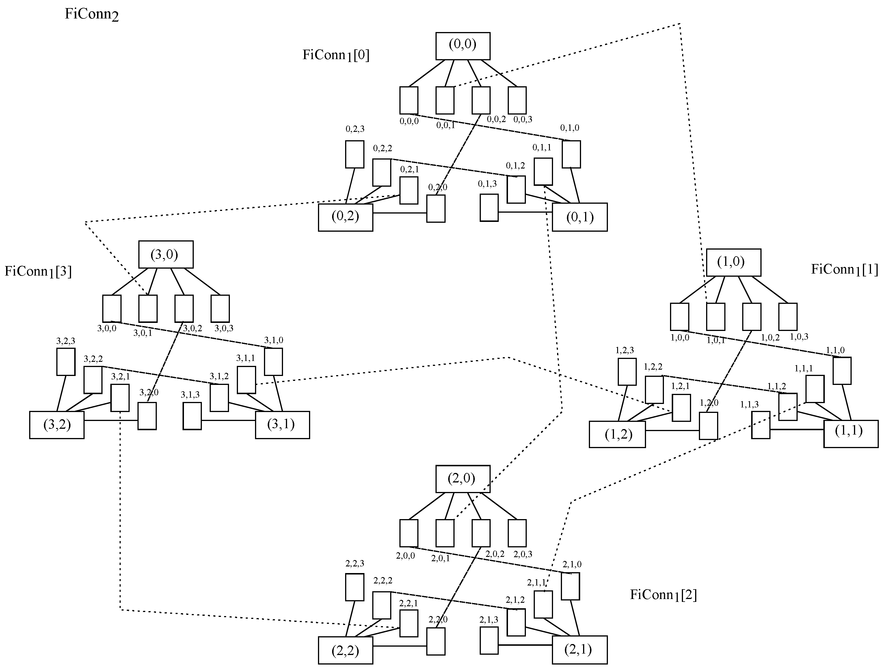
Negara et al. [57] compare BCube and DCell, obtaining better speed in data transmission for the latter, although the former has better security and integrity because it is able to forward data completely without any failures. Cortes et al. [58] confront Fat Tree and BCube, with the outcome indicating that the latter obtains better results than the former.Al Makhlafi et al. [59] state that data center networks may be classified into two broad groups, such as switch-centric and server-centric, where switches are mainly responsible for routing and networking in the former, whilst servers aremainly accountable in the latter, which allows the use of commodity switches [60]. Examples of the former are fat tree and leaf and spine, whereas instances of the latter are FiConn, DCell and BCube.

Yao et al. [61] carry out a comparative analysis among several well-known data center network topologies, such as Multi-tiered, Fat Tree, Flattened Butterfly, Camcube and BCube, regarding a variety of metrics, such as scalability, path diversity, hop count, throughput and cost, finding that different topologies scale differently for various metrics and concluding that designers must consider maximizing certain features whilst minimizing cost and power. Touihri et al. [62] propose a camcube design (k-ary n-cube) following the SDN paradigm such that the control plane is hosted in an SDN controller and including QoS into the decision-making process. After running several simulations using Mininet software, the results obtained are better than those attained with the shortest-path approach regarding packet error rate and latency.

Daryin et al. [63] undertake a comparison among diverse topologies for InfiniBand networks, such as tori, hypercube, Dragonfly, Flattened Butterfly and Slim Fly, and their results seem interesting in the field of data center networks. After having executed the necessary simulations, they conclude that the best outcome is obtained by Flattened Butterfly and a combination of this with Slim Fly.Rao et al. [64] carry out a comparison among different topologies for Network-on-Chip (NoC), such as Dragon Fly, Flattened Butterfly, Torus topology and Mesh topology; their results may be extrapolated to data center networks. Those comparisons were made with diverse figures of trade-offs, such as packet latency, network latency, throughput change and hop average; the authors concluded that Torus topology is the most efficient one for being adaptive in nature as well as for having less latency and time complexity.

Azizi et al. [65] compare a novel DCCube design with fat tree, Flattened Butterfly, BCube and SWCube, where the former achieves both higher performance and lower cost consideringthe number of switches, server NICs, server CPUs and cabling. Furthermore, Aguirre et al. [66] propose a greedy forwarding strategy that is independent of the network topology in place and obtains acceptable results, whilst Mohamed et al. [67] present average networking equipment power consumption for different topologies, showing that fat tree, leaf and spine, BCube and DCell obtain the highest outcome.In terms of creating a specific coefficient to measure performance in a data center, most efforts have been focused on energy efficiency. For instance, Sego et al. [68] come up with a metric called Data Center Energy Productivity (DCeP) as the ratio of useful work produced to the energy consumed to get that work done. Likewise, Santos et al. [69] propose a metric called Perfect Design Data Center (PDD) as a redefinition of Energy Usage Effectiveness Design (EUED), which reflects the efficiency in the power consumption.

Basically all the papers devoted to efficiency in data centers are focused on evaluation metrics about energy efficiency. In this sense, Shao et al. [70] make a review of energy efficiency evaluation metrics, combining energy conservation and eco-design, whilst Levy et al. [71] examine performance as a combination of productivity, efficiency, sustainability and operations. Kumar et al. [72] establish power usage effectiveness (PUE) as the metric to measure efficiency and study different machine learning techniques so as to make accurate predictions. Furthermore, Brocklehurs [73] proposes other usage effectiveness measurements, such as carbon (CUE) and water (WUE), along with a coefficient of performance (CoP) defined as the ratio of useful cooling provided to the energy input, where efficiency grows as the coefficient rises. Eventually, Reddy et al. [74] expose a systematic overview of data center metrics divided into categories such as energy efficiency, cooling, greenness, performance, thermal and air management, network, storage, security and financial impact. Among these metrics, a green energy coefficient (GEC) is defined as a percentage represented by green energy compared to the total energy consumed.

In summary, this section has been devoted to comment on relevant related work, where different papers have been presentedand diverse comparisons have been carried out among the most common data center network topologies, such as fat tree, leaf and spine, k-ary n-cube, BCube, DCell, FiConn, Flattened Butterfly, DragonFly and SlimFly, to quote the main ones. In those papers, a lot of metrics have been utilized so as to rate the different topologies by means of undertaking various tests, such as network size, bisection bandwidth, cost, throughput, latency, load balancing, mean time to failure or resilience to failure. However, the contribution of this paper is not to repeat those tests but to craft a new coefficient to obtain balance between performance and simplicity as defined in the terms exposed in the introduction. The goal herein is to be able to obtain a valuable figure in order to help the decision-making process when it comes to selecting a certain data center network architecture among a range of topologies, where each one may present different features, and that will be the target in the rest of the paper.

4. Coefficient Proposed to Obtain Balance between Performance and Simplicity

The coefficient proposed to measure efficiency of the different network topologies proposed for data centers needs to take into account both performance and simplicity of use along with maintenance in a way to achieve a trade-off between them. Regarding the former, it is measured by means of the average distance among nodes, whereas the latter it is stated as the average number of links per node (its degree) for graph-like designs, or otherwise, the average number of links per device (considering both nodes and switches) for tree-like designs.

Anyway, both averages should be as small as possible in order to obtain both performance and simplicity, such that the smaller the coefficient, the better. Regarding the average distance among nodes, it is going to be measured as the average number of hops between all pairs of nodes and denoted as $\alpha$. With respect to the average number of links per device, it is going to be measured as stated above and described as $\beta$.

Putting everything together, the coefficient proposed is going to be obtained by multiplying both averages, namely, $\alpha \times \beta$. In this sense, the lower the result obtained, the better the combination of both factors; hence, better balance between performance and simplicity will be attained. That is why the coefficient is branded $\eta$, which is the Greek letter used in physics and engineering for efficiency. Therefore, it may be said that (1) defines $\eta$.

$$\eta =\mathit{AvgDistance}\times \mathit{AvgLinks}=\alpha \times \beta$$

(1)

The main motivation of this paper is to calculate a coefficient involving a compromise between performance and simplicity—defined in the terms exposed in the introduction—in a way that such a value may help decide which data center network topology is more suitable, thus acting as a sort of tie-breaker to select among diverse interesting options. Therefore, this coefficient is just another tool for making the decision as to which data center is more convenient among diverse options along with other tests related to throughput, latency, cost or robustness.

As a practical-use case, let us focus on the situation exposed in the first two paragraphs of Section 3, which is devoted to related work. In the first one, it is stated that after the analysis carried out on reliability and survivability, BCube is the most robust design regarding link failures, whereas DCell isthe most robust regarding switch failures. Likewise, in the second one, it is claimed that after the tests were undertaken, BCube provided better security and data integrity, whilst DCellprovided better speed in data transmission. Hence, the coefficient proposed may act as a tie-breaker for the selection of the data center network architecture, as it presents a compromise between performance and simplicity for each of the possible options available.

5. Developing Some Typical Use Cases

After having presented some instances of network topologies fit for data centers along with the definition of coefficient $\eta$, some typical use cases are going to be developed, taking into account that the number of nodes that will be up and runningis considered to be small to medium. In order to cope with this, a limit of 16 nodes per topology is going to be imposed, although smaller numbers are going to be exposed as well. Basically, a systematic approach by means of powers of two is going to be described in the following subsections. Additionally, another one is going to be devoted to fit those designs not matching any power of two, and eventually, a further one is dedicated to some other commonly used network topologies in larger data centers.

Regarding the calculations for all topologies, the average number of hops has been undertaken by first selecting a given end host and, in turn, adding up the number of hops to reach all its peers within the topology and dividing into the count of such peers. Otherwise, the average number of links has been carried out by adding up the links of each device, no matter if they are end hosts or switches, and dividing into the count of all those devices.

It is to be reminded that data center network topologies need to avoid single points of failure in critical points; thus, redundancy is a must. From that point of view, single hub and spoke topologies have not been taken into account, whilst redundant hub and spoke topologies have been included into this study. Further, it happens that the definition of this coefficient gives advantage to topologies with fewer average links, which may benefit non-redundant topologies against redundant ones. Hence, in order to avoid this situation, this coefficient was restricted only to redundant topologies. On the other hand, topologies with more than two redundant links are penalized against topologies with just two of such links, although those cases are not considered herein, as the most common layout is to have just two redundant devices.

5.1. One Node within the Topology

This is a trivial case as the number of nodes is $2^0=1$. Then, there is just one single node in the topology; thus, obviously there are no alternative topology designs for this condition, neither for tree-like designs nor for graph-like ones. Hence, the average distance among nodes and the average number of links per node are both zero. Therefore, as $\alpha =0$ and $\beta =0$, then $\eta =\alpha \times \beta =0$ for both types of topologies, as stated in

Table 1. Values of $\eta$ for the case of $2^0=1$ node.

Type	Instance	$\mathit{\alpha }$	$\mathit{\beta }$	$\mathit{\eta }=\mathit{\alpha }\times \mathit{\beta }$
Tree-like	none	0	0	0
Graph-like	none	0	0	0

.

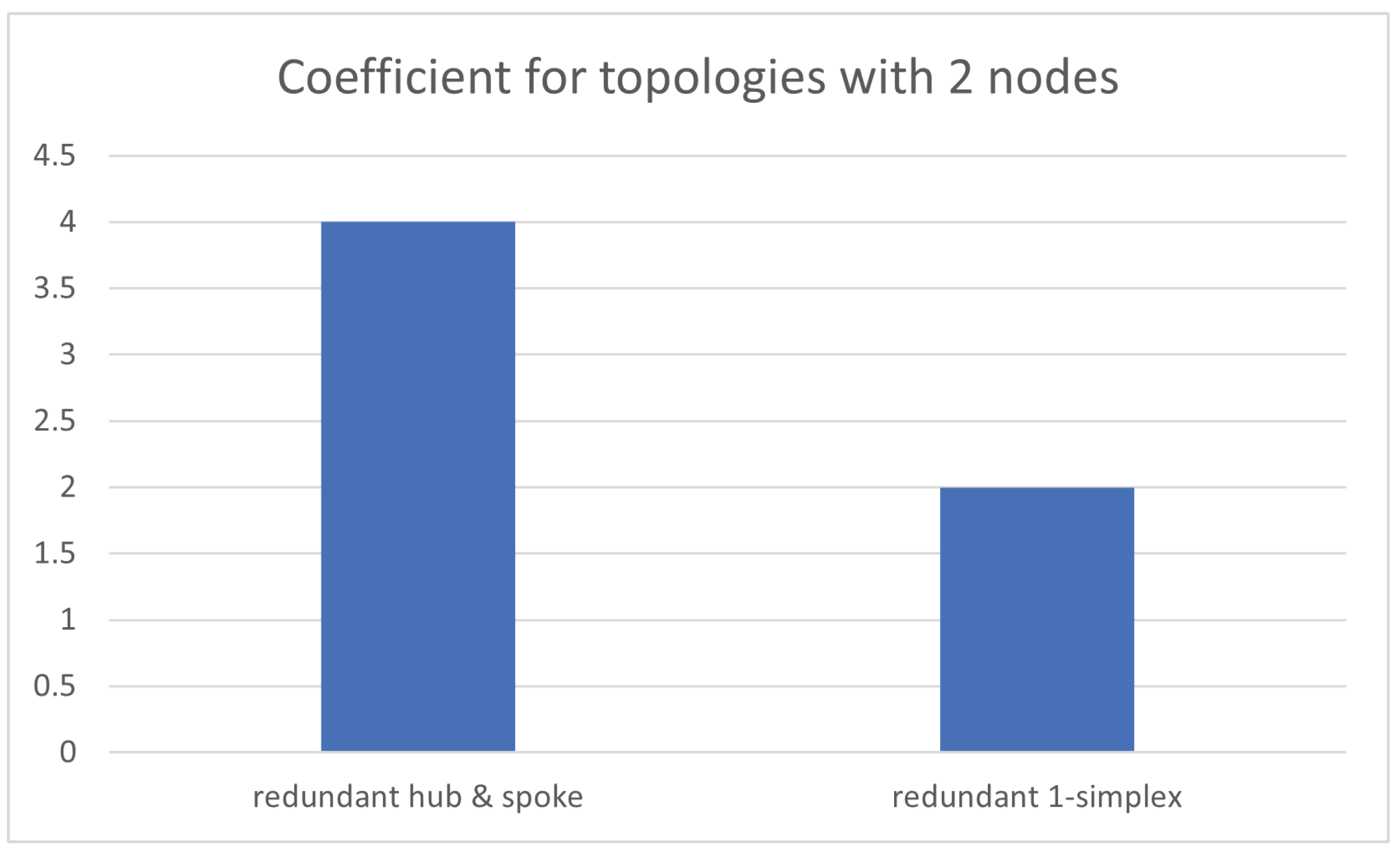
5.2. Two Nodes within the Topology

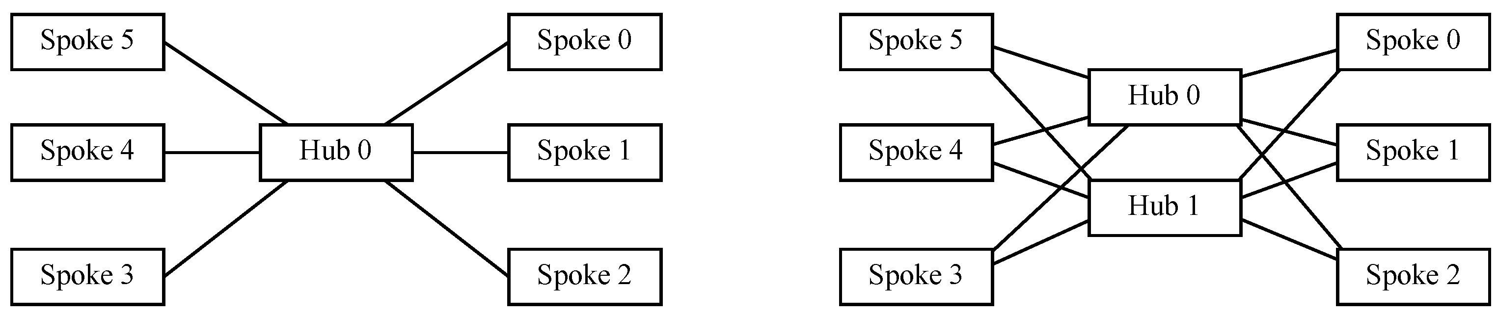
In this case, the number of nodes is $2^1=2$. This is straightforward, as the only tree-like option is hub and spoke; thus, both nodes act as spokes which are linked together through a hub, whereas the only graph-like option is a direct link among nodes, provided no multiple links are considered. However, as redundancy needs to be considered when dealing with Data Center Network (DCN) architectures, then a redundant hub and spoke will be considered for the tree-like case, whereas a double direct linkbetween both nodes will be done for the graph-like case, which accounts for a redundant 1-simplex.

Hence, on the one hand, the average distance among nodes forredundant hub and spoke is $\alpha =2$ because two hops are needed to go from one node to the other, whilst it is $\alpha =1$ inredundant 1-simplex because just one hop is necessary to move to the other node. On the other hand, the average number of links for tree-like environments is two for both hubs and both spokes so as to build up the redundant hub and spoke, thus accounting for $\beta =2$, whereas it is also $\beta =2$ for graph-like environments, as each node hastwo redundant links towards the other one. Therefore, for the tree-like design, $\eta =\alpha \times \beta =2\times 2=4$, whilst for the graph-like design, $\eta =1\times 2=2$, as stated in

Table 2. Values of $\eta$ for the case of $2^1=2$ nodes.

Type	Instance	$\mathit{\alpha }$	$\mathit{\beta }$	$\mathit{\eta }=\mathit{\alpha }\times \mathit{\beta }$
Tree-like	redundant hub and spoke	2	2	4
Graph-like	redundant 1-simplex	1	2	2

.

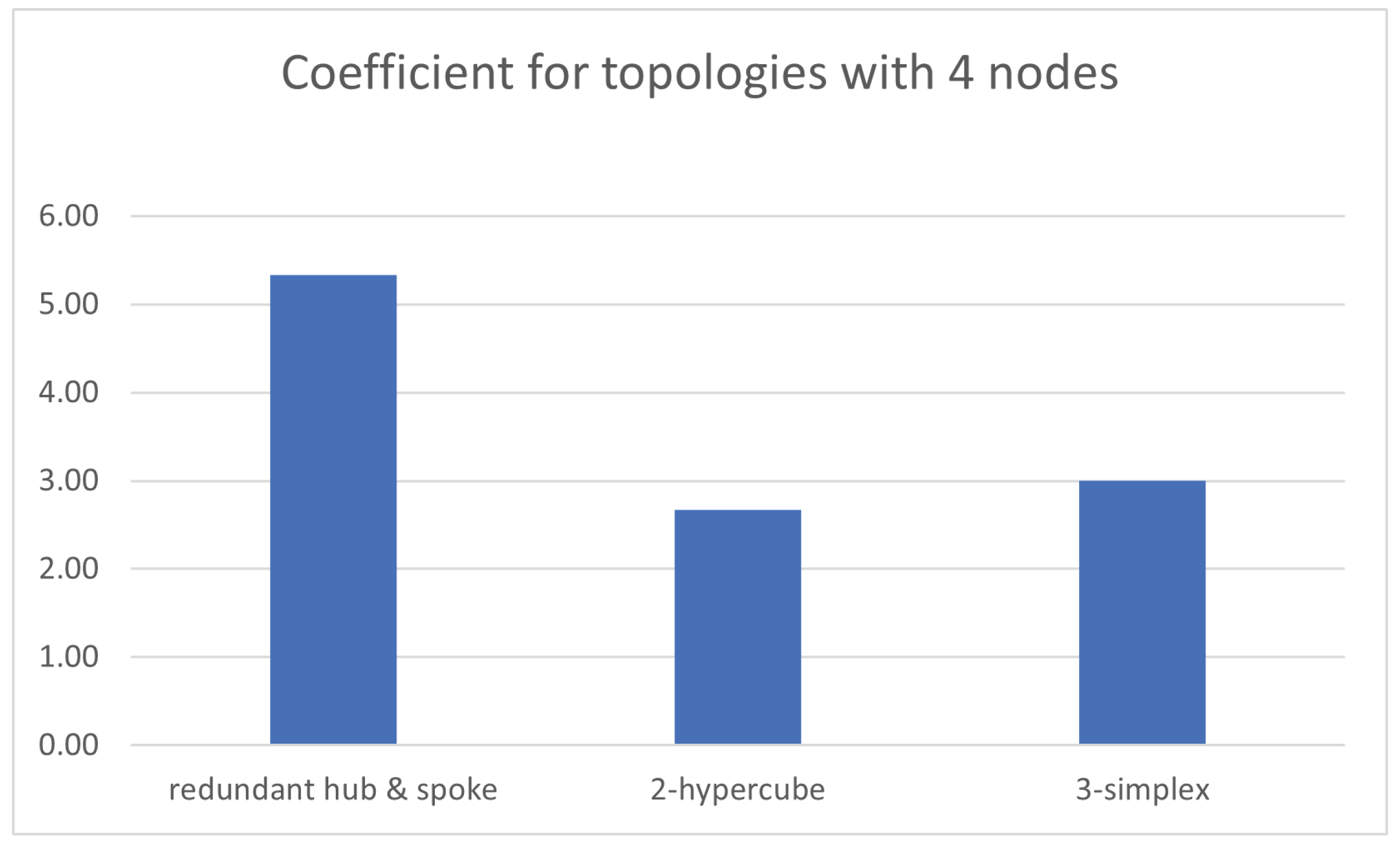
5.3. Four Nodes within the Topology

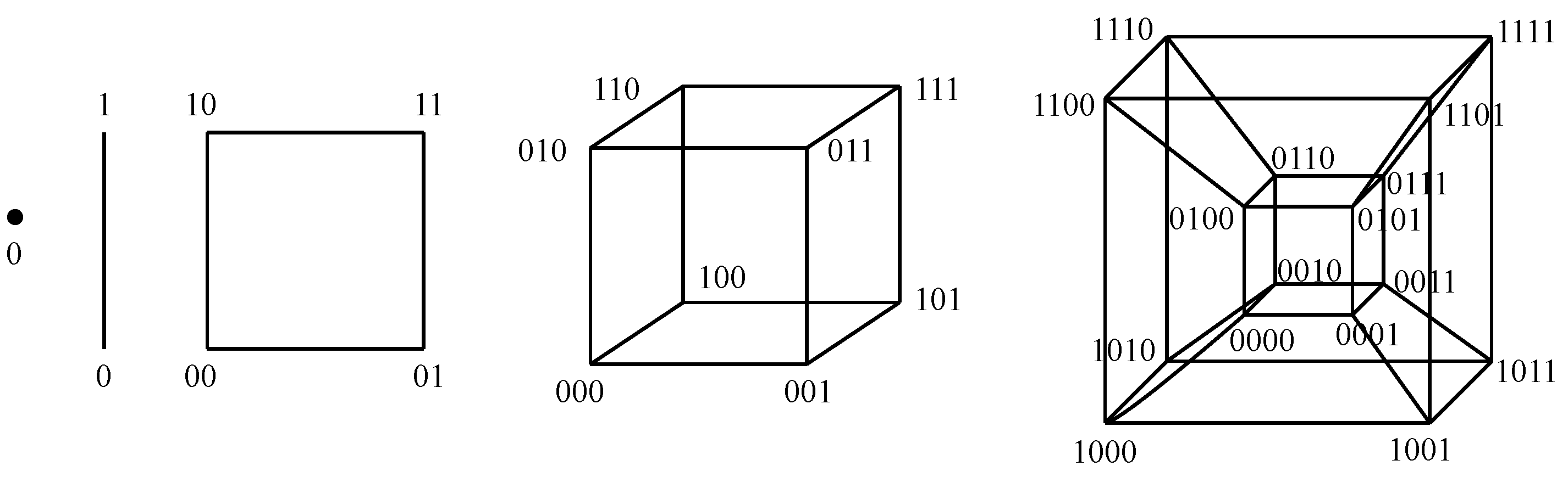
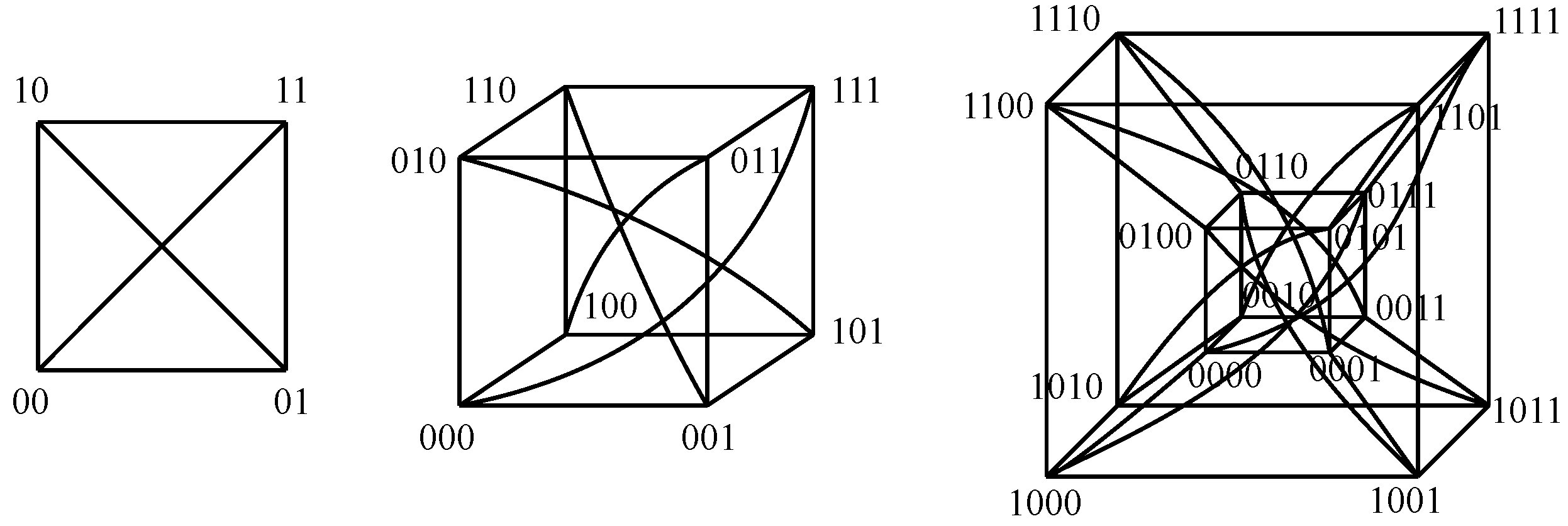
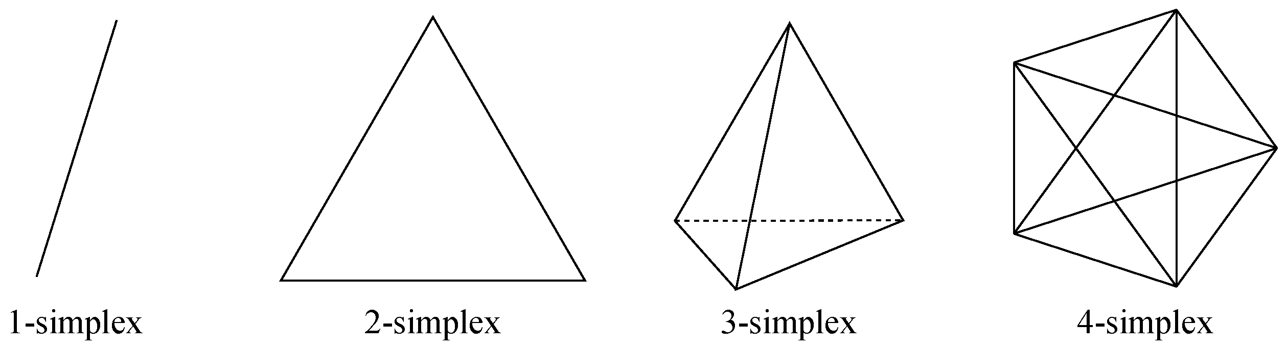
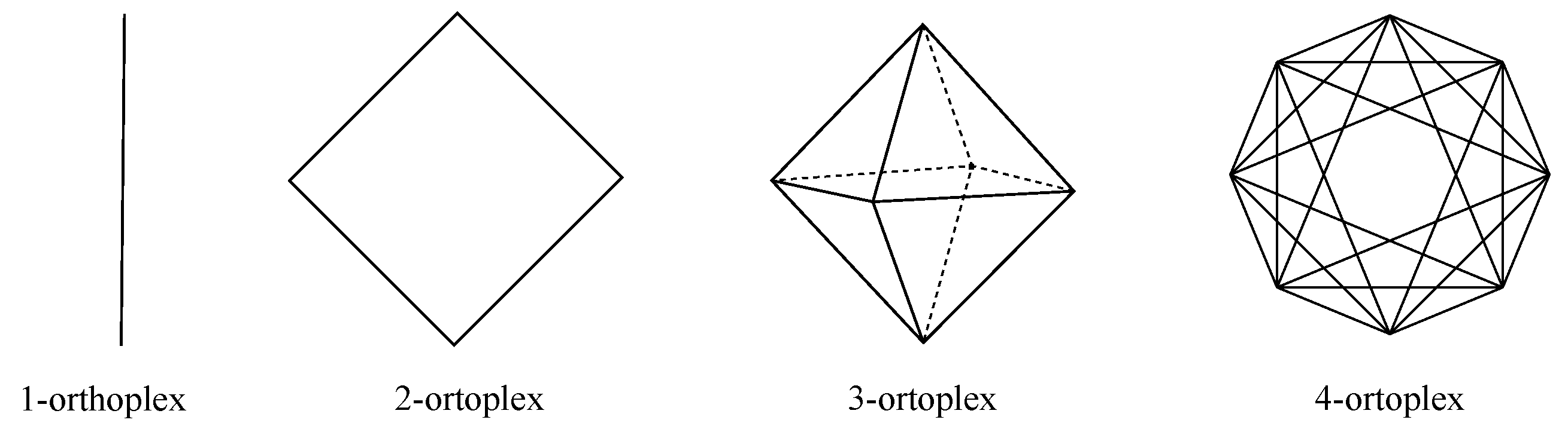
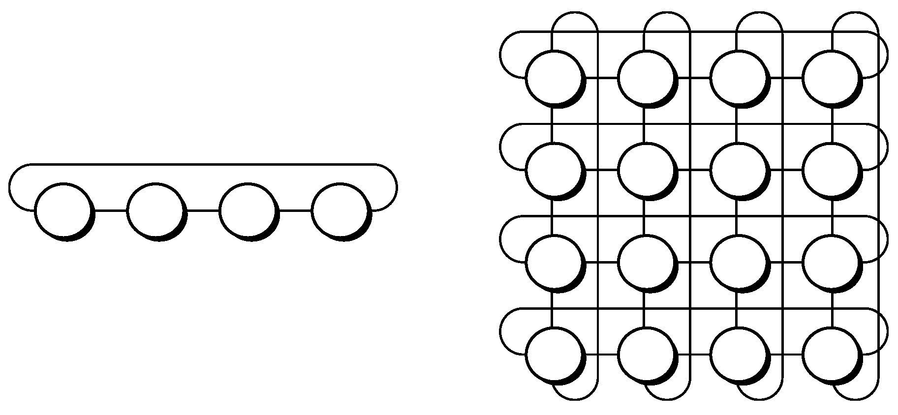
Now, the number of nodes is $2^2=4$. Regarding tree-like options, it is possible to deploy a redundant hub and spoke, which is equivalent to a leaf and spine with four leaves and two spines. With respect to graph-like choices, it is possible to deploy a square, which accounts for a 2-hypercube, that being equivalent toboth a 2-orthoplex and a 2-ary 2-cube, or otherwise, to deploy a full-mesh, which represents a 3-simplex, that being equivalent toboth a folded 2-hypercube and a Hamming graph $H_2(2,1)$.

Table 3. Values of $\eta$ for the case of $2^2=4$ nodes.

Type	Instance	$\mathit{\alpha }$	$\mathit{\beta }$	$\mathit{\eta }=\mathit{\alpha }\times \mathit{\beta }$
Tree-like	redundant hub and spoke	2	2.67	5.33
Graph-like	2-hypercube	1.33	2	2.66
	3-simplex	1	3	3

exhibits the relevant values of $\eta$ for each instance proposed.

Focusing on tree-like designs, the $\alpha$ value for redundant hub and spoke is two hops among any pair of nodes, whilst it results in $\beta =(4\times 2+2\times 4)/(4+2)=2.67$ as there are four spokes with two links (one connection to each hub) and two hubs with four links each (one connection to each spoke).

On the other hand, centering on graph-like designs, 2-hypercube presents two nodes at one hop and another node at two hops, resulting in $\alpha =(2\times 1+1\times 2)/(2+1)=1.33$ and $\beta =2$ as each node has two links, whereas 3-simplex results in $\alpha =1$ because all nodes are only one hop away, and $\beta =3$ as all nodes have just three links.

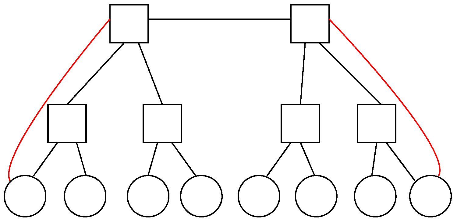
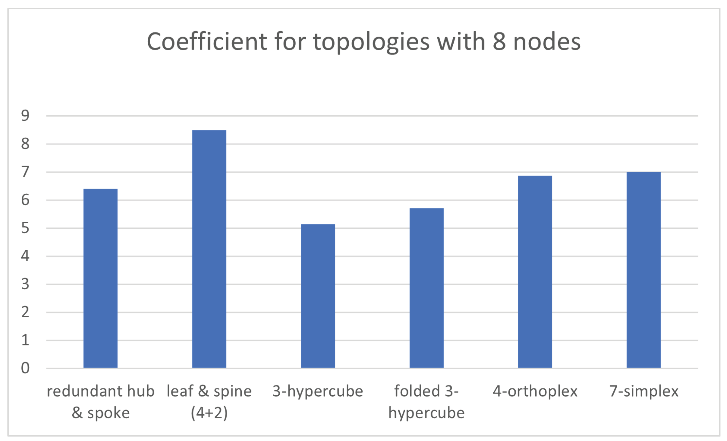
5.4. Eight Nodes within the Topology

At this point, the number of nodes is $2^3=8$. Regarding tree-like choices, it is possible to deploy a redundant hub and spoke and a leaf and spine with two spines and four leaves, where two hostsare connected to each of them. Otherwise, with respect to graph-like alternatives, it is possible to go for a 3-hypercube, a folded 3-hypercube, a 4-orthoplex and a 7-simplex.

Table 4. Values of $\eta$ for the case of $2^3=8$ nodes.

Type	Instance	$\mathit{\alpha }$	$\mathit{\beta }$	$\mathit{\eta }=\mathit{\alpha }\times \mathit{\beta }$
Tree-like	redundant hub and spoke	2	3.2	6.4
	leaf and spine	3.71	2.29	8.5
Graph-like	3-hypercube	1.71	3	5.13
	folded 3-hypercube	1.43	4	5.72
	4-orthoplex	1.14	6	6.86
	7-simplex	1	7	7

exhibits the relevant values of $\eta$ for those instances.

With regards to the tree-like designs, redundant hub and spoke presents a steady value of $\alpha =2$ as all nodes are two hops away, whilst leaf and spine has an $\alpha =(1\times 2+6\times 4)/(1+6)=3.71$, because taking a given node, there is another node hanging on the same leaf and the other six nodes hang on different leaves. On the other hand, it results in $\beta =(2\times 8+8\times 2)/(2+8)=3.2$ for the former, as the two hubs are connected to the eight spokes and the other way around, whereas ityields $\beta =(8\times 1+4\times 4+2\times 4)/(8+4+2)=2.29$ for the latter. This outcome is because the eight nodes are connected to their corresponding leaves upwards, whilst each of the four leaves are connected to two nodes downwards and two spines upwards and each of the two spines are connected to all four leaves downwards.

Furthermore, the selected graph-like designs present the following values: $\alpha =(3\times 1+3\times 2+1\times 3)/(3+3+1)=1.71$ and $\beta =3$ for the first one, $\alpha =(4\times 1+3\times 2)/(4+3)=1.43$ and $\beta =4$ for the second one, $\alpha =(6\times 1+1\times 2)/(6+1)=1.14$ and $\beta =6$ for the third one, whereas $\alpha =1$ and $\beta =7$ for the fourth one.

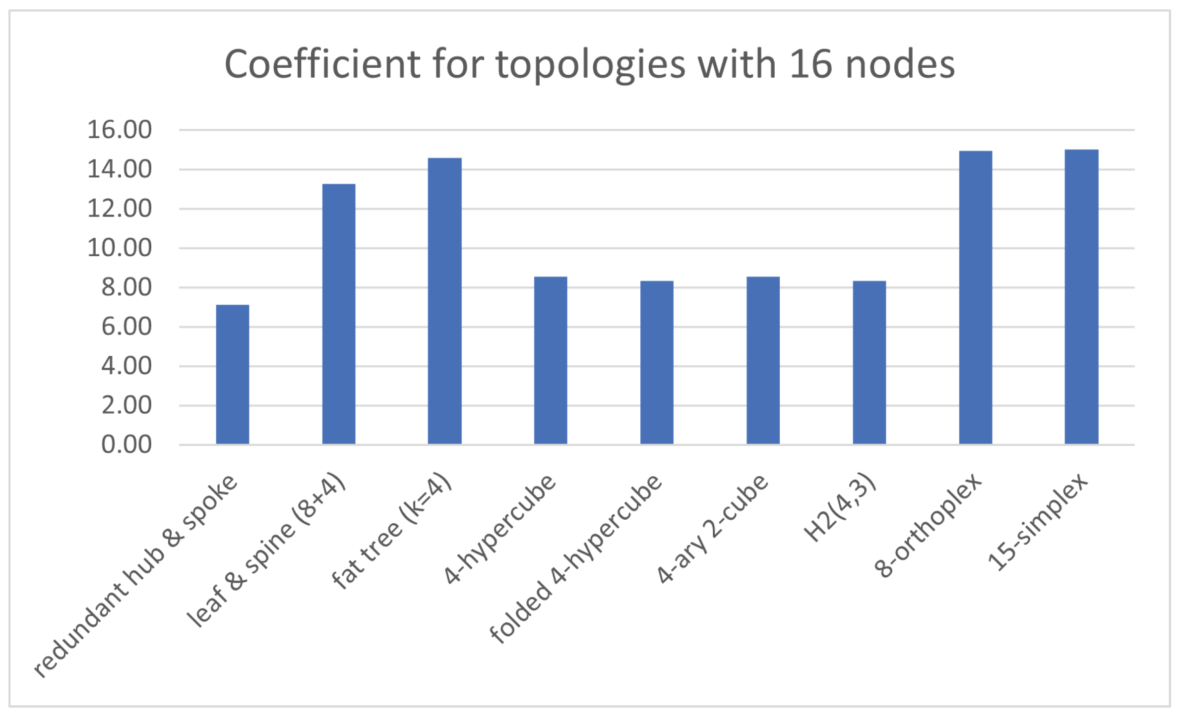
5.5. Sixteen Nodes within the Topology

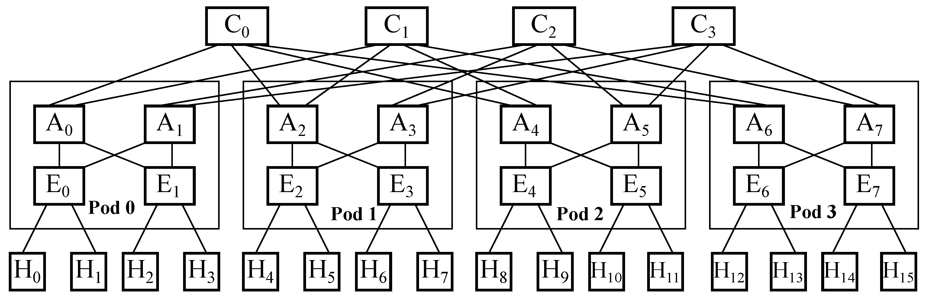
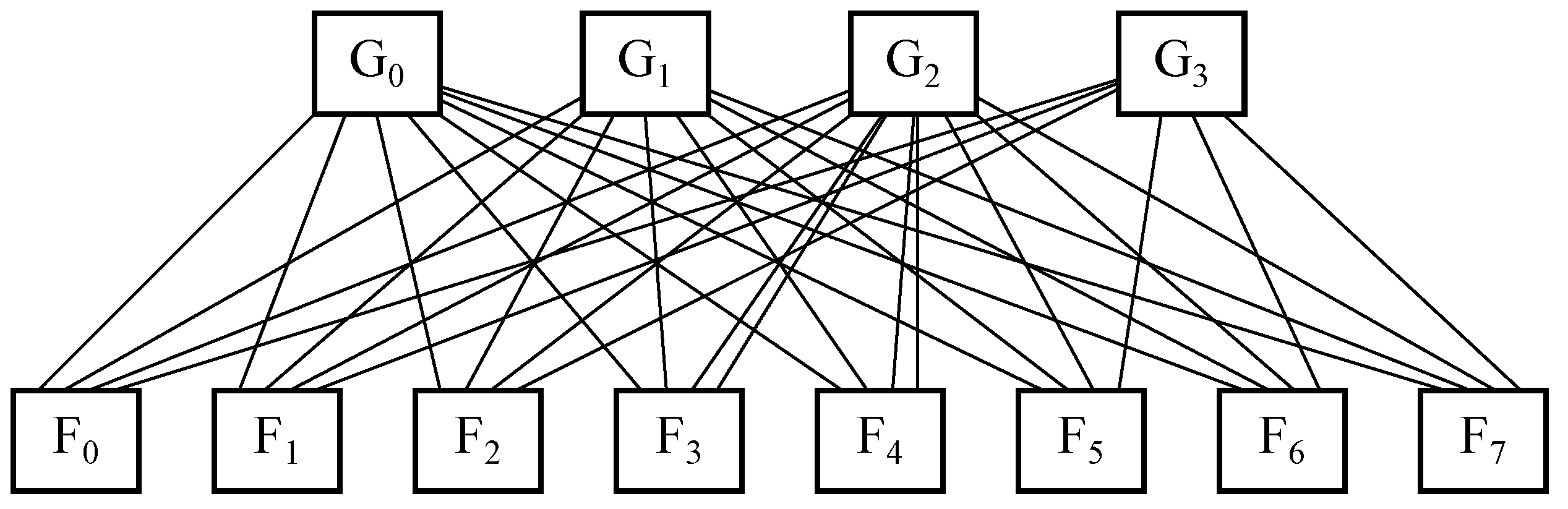
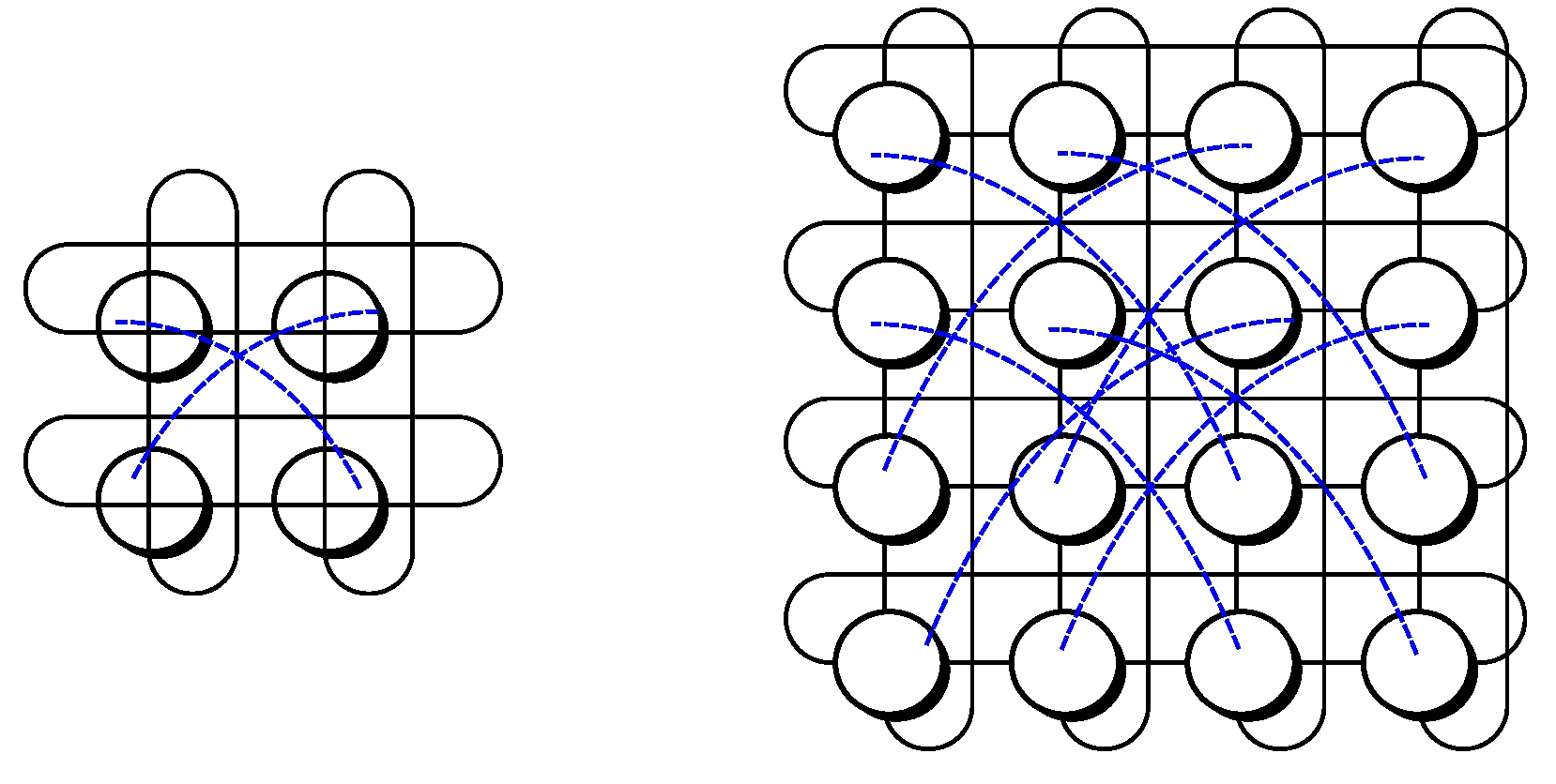
The following case exhibits a number of nodes $2^4=16$. With respect to tree-like options, it is possible to deploy a redundant hub and spoke, a leaf and spine with four spines and eight leaves, where two hostsare connected to each of them, and even a fat tree with $k=4$,which accounts for four core switches, eight aggregation switches and eight edge switches, where two hostsare connected to each one of those. Otherwise, regarding graph-like alternatives, it is possible to go for a 4-hypercube, a folded 4-hypercube, a 4-ary 4-cube, a Hamming graph $H_2(4,3)$, an 8-orthoplex and a 15-simplex.

Table 5. Values of $\eta$ for the case of $2^4=16$ nodes.

Type	Instance	$\mathit{\alpha }$	$\mathit{\beta }$	$\mathit{\eta }=\mathit{\alpha }\times \mathit{\beta }$
Tree-like	redundant hub and spoke	2	3.56	7.12
	leaf and spine	3.87	3.43	13.27
	fat tree $(k=4)$	5.47	2.67	14.60
Graph-like	4-hypercube	2.13	4	8.52
	folded 4-hypercube	1.67	5	8.35
	4-ary 4-cube	2.13	4	8.52
	$H_2(4,3)$	1.67	5	8.35
	8-orthoplex	1.07	14	14.93
	15-simplex	1	15	15

exhibits the relevant values of $\eta$ for all those instances.

Focusing on the tree-like designs, redundant hub and spoke presents a steady value of $\alpha =2$, whereas leaf and spine has an $\alpha =(1\times 2+14\times 4)/(1+14)=3.87$, and fat tree has an $\alpha =(1\times 2+3\times 4+12\times 6)/(1+2+12)=5.47$. On the other hand, it results in $\beta =(2\times 16+16\times 2)/(2+16)=3.56$ for the first one, whereas $\beta =(16\times 1+8\times 6+4\times 8)/(16+8+4)=3.43$ for the second one, and $\beta =(16\times 1+8\times 4+8\times 4+4\times 4)/(16+8+8+4)=2.67$ for the third one.

Additionally, the chosen graph-like designs account for the following values: $\alpha =(4\times 1+6\times 2+4\times 3+1\times 4)/(4+6+4+1)=2.13$ and $\beta =4$ for the first one, $\alpha =(5\times 1+10\times 2)/(5+10)=1.67$ and $\beta =5$ for the second one, $\alpha =(4\times 1+6\times 2+4\times 3+1\times 4)/(4+6+4+1)=2.13$ and $\beta =4$ for the third one, $\alpha =(5\times 1+10\times 2)/(5+10)=1.67$ and $\beta =5$ for the fourth one, $\alpha =(14\times 1+1\times 2)/(14+1)=1.07$ and $\beta =14$ for the fifth one, and $\alpha =1$ and $\beta =15$ for the sixth one.

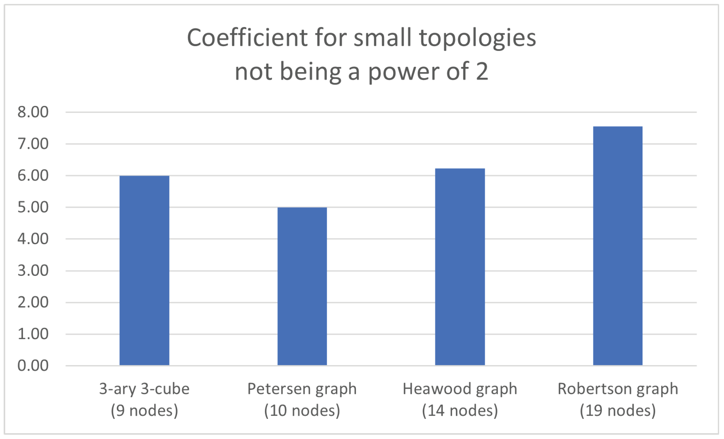
5.6. Other Numbers of Nodes within the Topology Not Being a Power of Two

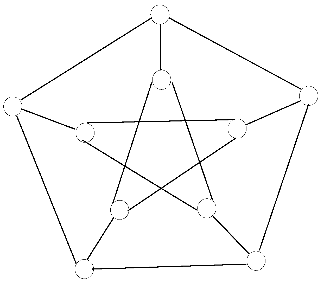
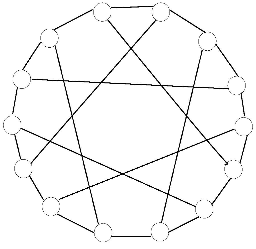
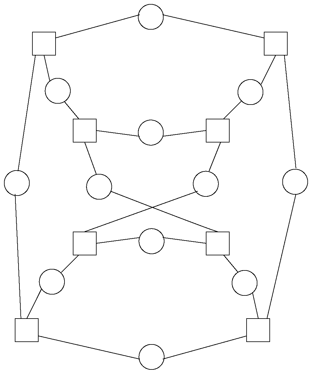
This additional case includes some topology layouts whose number of nodes is not a power of two, such as 3-ary 3-cube, Petersen graph, Heawood graph and Robertson graph, all of them being graph-like designs. As per the first one: $\alpha =(4\times 1+4\times 2)/(4+4)=1.5$ and $\beta =4$, whilst for the second one: $\alpha =(3\times 1+6\times 2)/(3+6)=1.67$ and $\beta =3$, whereas for the third one: $\alpha =(3\times 1+6\times 2+4\times 3)/(3+6+4)=2.08$ and $\beta =3$, while for the fourth one: $\alpha =(4\times 1+12\times 2+2\times 3)/(4+12+2)=2.08$ and $\beta =3$.

Table 6. Values for $\eta$ for nodes not being a power of 2.

Type	Instance	Nodes	$\mathit{\alpha }$	$\mathit{\beta }$	$\mathit{\eta }=\mathit{\alpha }\times \mathit{\beta }$
Graph-like	3-ary 3-cube	9	1.5	4	6
	Petersen graph	10	1.67	3	5
	Heawood graph	14	2.08	3	6.24
	Robertson graph	19	1.89	4	7.56

exposes the relevant values of $\eta$ for these instances.

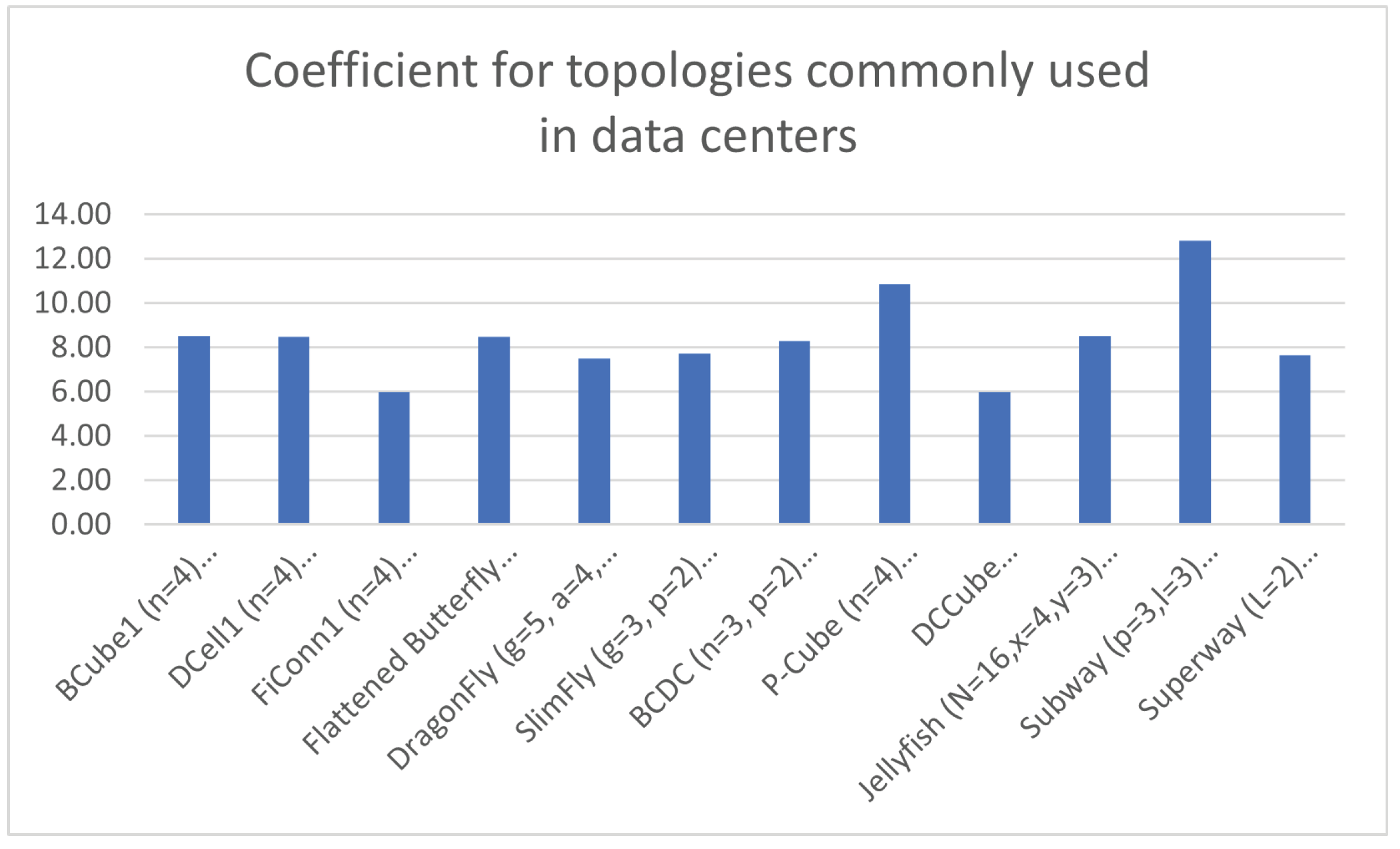
5.7. Some Other Commonly Used Network Topologies in Data Centers

In order to apply the aforementioned coefficient $\eta$ to obtain a balance between performance and simplicity to network topologies being employed in large data centers, the topologies exposed in Section 2.3 are going to be used to calculate the aforesaid coefficient $\eta$. This study is going to be made with the parameters exposed in that subsection that correspond to a data center with small to medium size. However, these parameters are higher in large deployments; hence, the use of coefficient $\eta$ may be applied the same way as exposed in this section, although the results may vary depending on the values taken for the corresponding parameters.

Anyway,

Table 7. Values of $\eta$ for other commonly used network topologies in data centers.

Type	Instance	Nodes	$\mathit{\alpha }$	$\mathit{\beta }$	$\mathit{\eta }=\mathit{\alpha }\times \mathit{\beta }$
Tree-like	BCube${}_1$ $(n=4)$	16	3.20	2.67	8.53
	DCell${}_1$ $(n=4)$	20	3.53	2.40	8.46
	FiConn${}_1$ $(n=4)$	12	3.00	2.00	6.00
	Flattened Butterfly $(n=3)$	27	3.38	2.50	8.46
	DragonFly $(g=5,a=4,p=2)$	40	3.74	2.00	7.49
	SlimFly $(g=3,p=2)$	36	3.31	2.33	7.73
	BCDC $(n=3,p=2)$	12	3.45	2.40	8.29
	P-Cube $(n=4)$	32	4.26	2.55	10.84
	DCCube $(k=1,m=4,h=1,c=2)$	16	3.60	1.67	6.00
	Jellyfish $(N=16,x=4,y=3)$	16	4.27	2.00	8.53
	Subway $(p=3,l=3)$	6	3.20	4.00	12.80
	Superway $(L=2)$	8	3.29	2.33	7.67

exposes the values for such a coefficient $\eta$ regarding a compromise between performance and simplicity, where the parameters of each topology arealso shown, along with the number of nodes involved with those parameters, followed by the values for performance $\left(\alpha \right)$ and simplicity $\left(\beta \right)$ for those specific parameters.

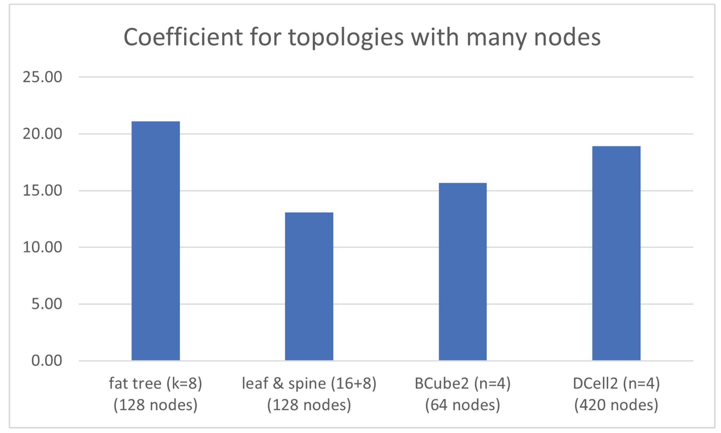
Additionally,

Table 8. Values of $\eta$ for network topologies in data centers with larger numbers of nodes.

Type	Instance	Nodes	$\mathit{\alpha }$	$\mathit{\beta }$	$\mathit{\eta }=\mathit{\alpha }\times \mathit{\beta }$
Tree-like	fat tree $(k=8)$	128	5.72	3.69	21.11
	leaf and spine (128 hosts)	128	3.89	3.37	13.10
Recursive	BCube${}_2$ $(n=4)$	64	4.57	3.43	15.67
	DCell${}_2$ $(n=4)$	420	5.92	3.20	18.94

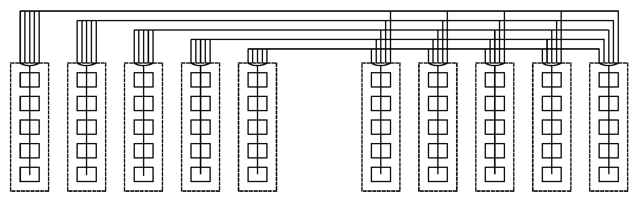
exhibits the values for coefficient $\eta$ when the number of nodes involved in diverse data center network topologies is increased. For this case, fat tree has been selected with parameter $k=8$, which contains 128 hosts withjust 1 port, along with 32 edge switches, 32 aggregation switches and 16 core switches, where all of themhave 8 ports. Further, leaf and spine has also been set up to include 128 hosts with 1 port by taking 16 leaves and 8 spines, all of them being switches with 16 ports.

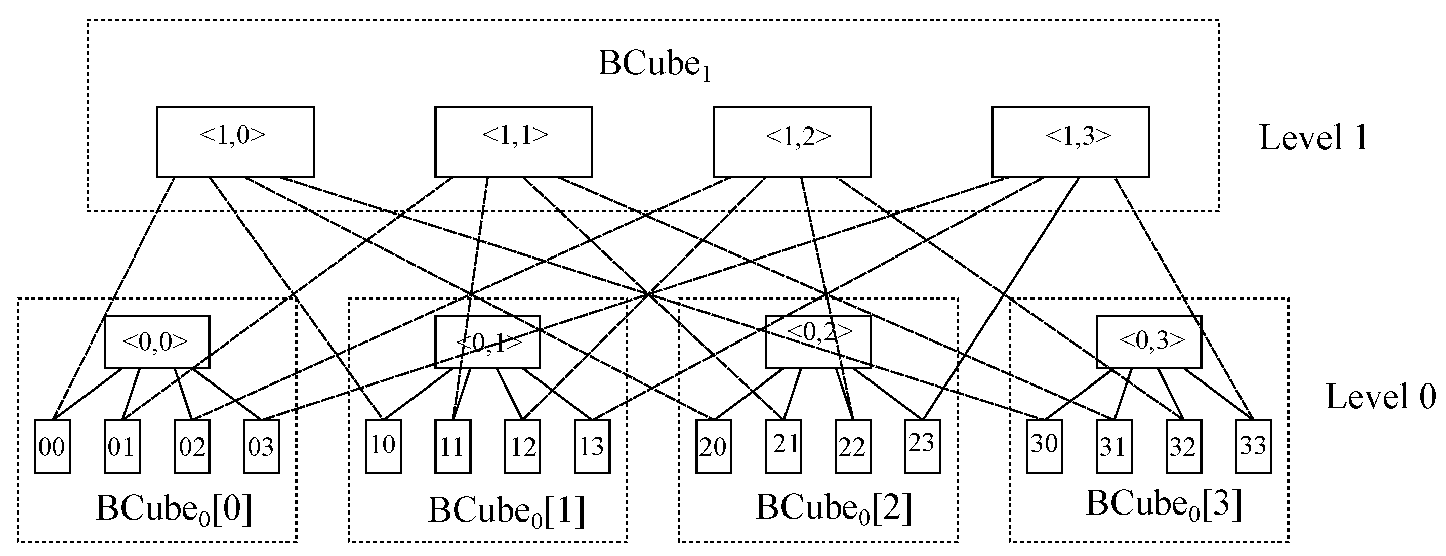
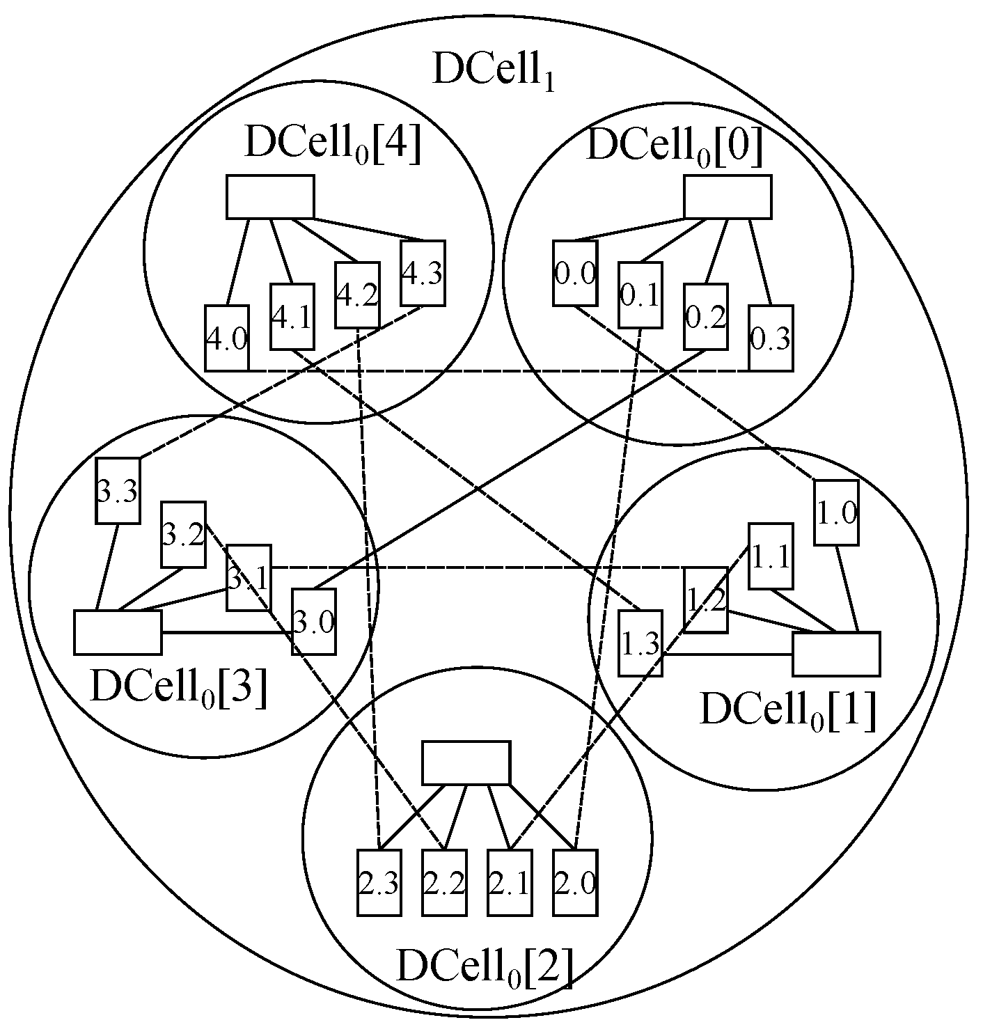
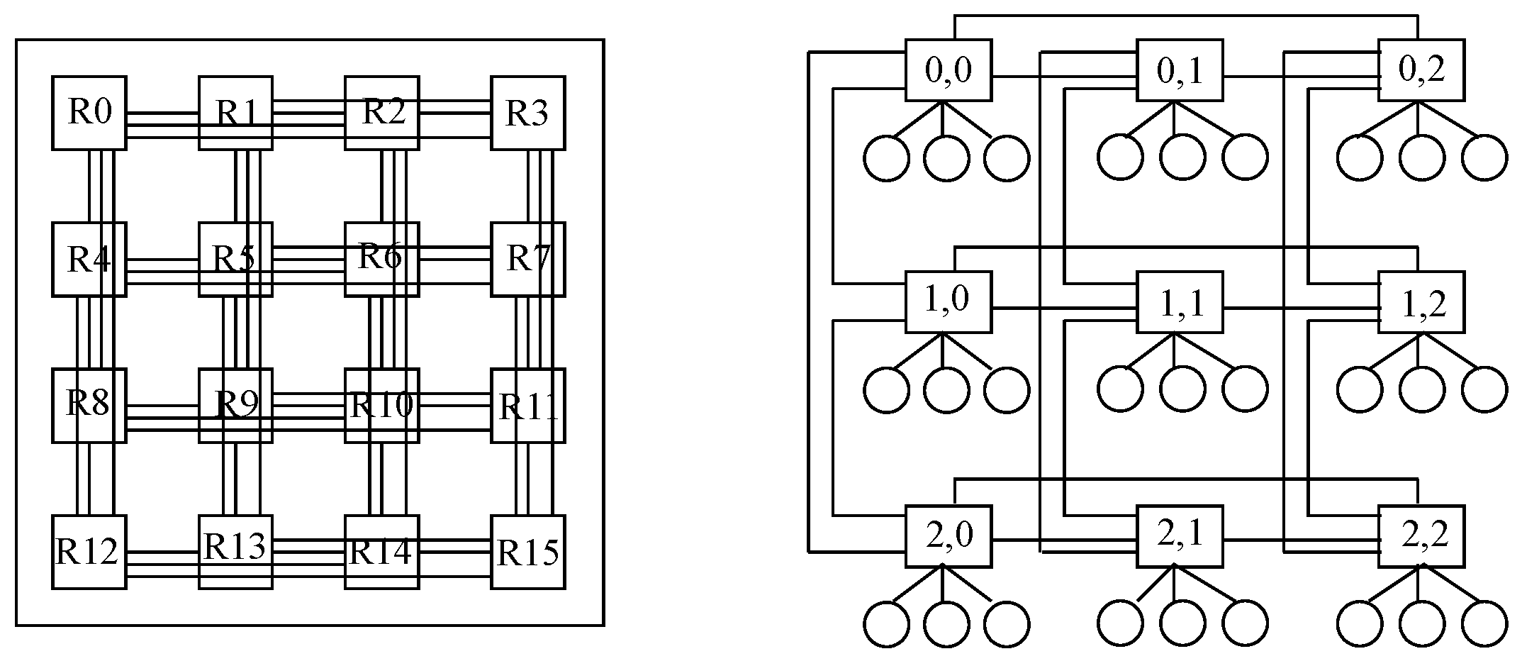
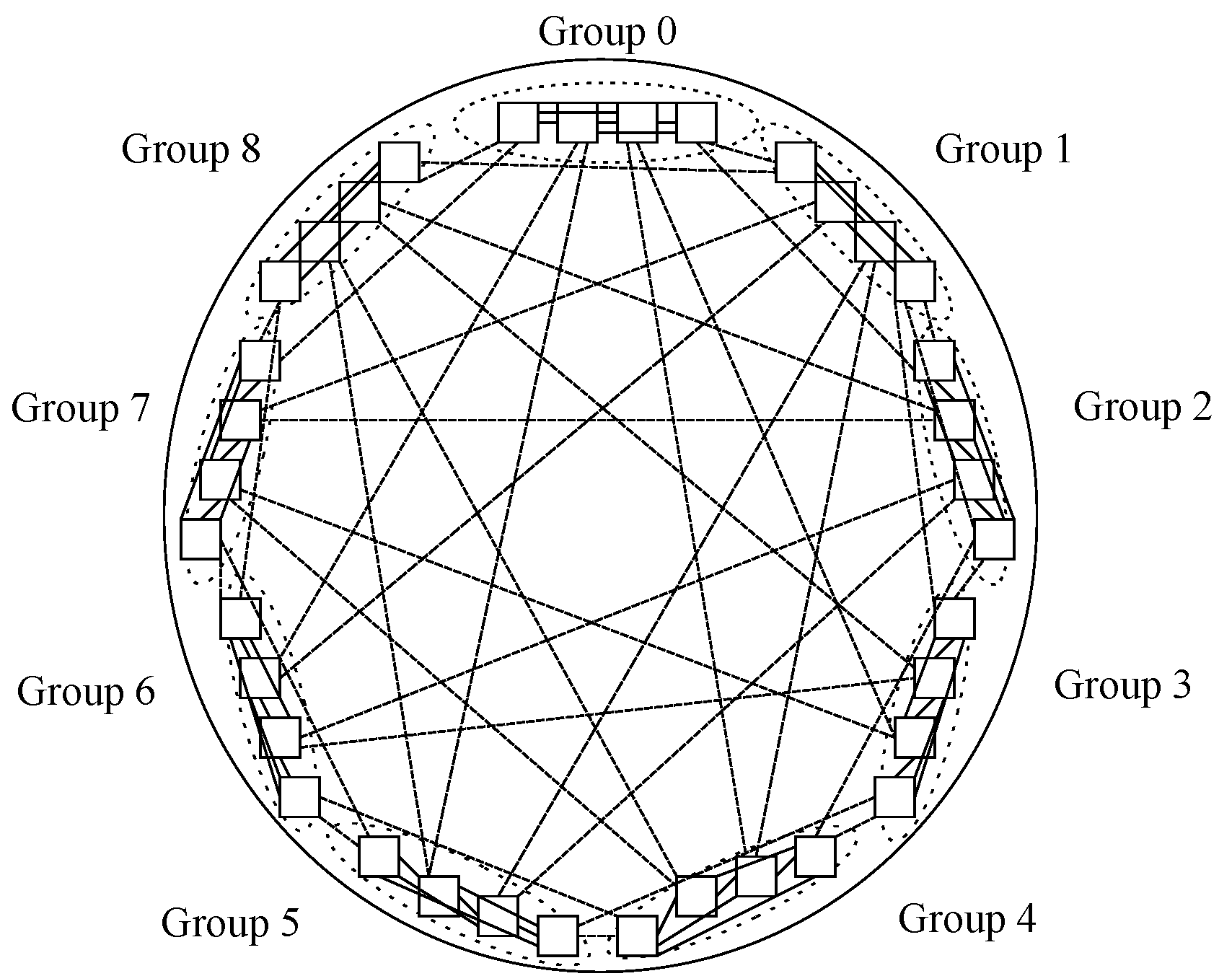
Furthermore, BCube${}_2$ with $n=4$ is chosen, whichcontains 64 hosts with 3 ports and 48 switcheswith 4 ports. It is to be noted that a third ofthose switches belong tothe 16 level-0 cells within this topology, with 4 nodes hanging on each of those, another third is located in 4 level-1 cells, with 4 level-0 cells hanging on each of these, and the other third one is situated within the level-2 cell, with 4 level-1 cells hanging on each of them. Moreover, DCell${}_2$ with $n=4$ is also selected, which holds 420 hosts with 3 ports and 105 switches with 4 ports. It is to be said that those switches are distributed into 21 DCell${}_1$,where each of themhas 5 switches, such that each of those switches accounts for a DCell${}_0$, which in turn is furnished by 4 connected nodes.

6. Discussion about the Results Obtained

The study carried out above, from the point of view of arithmetic, presents some conclusions to be taken into account. To start with, the values of $\eta$ obtained for tree-like designs are higher than those for graph-like designs when it comes to $\alpha$, although regarding $\beta$ it is the other way around. In other words, the average number of hops is greater for tree-like instances because of the excess of links due to the switching hierarchy, whilst this hierarchical nature allows nodes to have no interconnection with their peers, as those are undertaken among switches.

Further, the different topologies proposed for a given number of hosts result in higher values of $\eta$ as the number of redundant paths grows, which happens for both tree-like and graph-like designs. Focusing on the former, the redundant hub and spoke presents the lowest value, followed by leaf and spine, and finally, fat tree. Centering on the latter, partial mesh topologies attain lower values of $\eta$, although the values grow as the number of links rises, increasing to maximum values for full-mesh topologies.

Additionally, in tree-like designs, the average number of links among hosts increases with redundancy, whilst the average number of links per device decreases, resulting in $\eta$ going higher, which shows that the weight of $\alpha$ is bigger than $\beta$ in tree-like topologies. On the contrary, in graph-like designs, the average number of links among hosts decreases with redundancy, whereas the average number of links per device increases, resulting in $\eta$ going higher, which points out that the weight of $\beta$ is bigger than $\alpha$ in graph-like topologies.

Having said that, further research could add some correction factor in order to try to balance the opposite relationship between $\alpha$ and $\beta$ for both kinds of architectures when using the proposed expression of $\eta$.

On the other hand, the values of performance and simplicity achieved with the other commonly used network topologies typically employed in data centers, described in Section 2.3 and calculated in Section 5.7, are significantly lower than their counterparts analyzed in the previous subsections within Section 5 for similar or even higher numbers of nodes. The reason of this is because the interconnections among nodes are optimized related to fat tree or leaf and spine, thus not presenting a pure tree structure butdisplaying more direct connections among nodes in many cases, and additionally, several instances furnish nodes with multiple ports to connect to different destinations.

Basically, large data centers employ optimized data center network topologies in order to attain shorter paths among nodes while facilitating scalability by means of setting the appropriate values for the parameters involved in such topologies. Therefore, it may be said that the coefficient proposed herein still stands for large scale topologies.

In order to facilitate discussion, the results obtained in Table 2, Table 3, Table 4, Table 5, Table 6, Table 7 and Table 8 have been graphically represented. It is to be said that Table 1 offers a trivial case where coefficient $\nu$ is null, so it has not been drawn. On the other hand, the correspondence of tables and figures is the following: Table 2 goes with Figure 26, Table 3 does with Figure 27, Table 4 does with Figure 28, Table 5 does with Figure 29, Table 6 goes with Figure 30, Table 7 goes with Figure 31, and Table 8 goes with Figure 32.

In summary, by reviewing the results obtained in Table 1, Table 2, Table 3, Table 4 and Table 5 for the coefficient proposed herein, namely $\eta$, it may be seen that the values attained for both tree-like and graph-like cases increase as the number of nodes rises. Further, the results shown in Table 6 are reasonable comparing the values achieved with those shown in the previous tables according to the number of nodes, as they are all within the same range.

Regarding the other commonly used data center network topologies presented in Table 7, the results are also coherent according to the amount of nodes included in each topology compared to those seen in the aforesaid tables. It is to be taken into account that Table 7 represents topologies where the number of nodes cover a wide range of values, as each topology has its own specifications. Nonetheless, most of the results obtained for $\eta$ are located in the lower range in the previous tables despite Table 7 instances having a larger number of nodes in many cases.

Therefore, it seems that this coefficient $\eta$ offers significant results for data center network topologies focused onsmall deployments. However, as exposed in previous sections, this coefficient is just another tool to select the most convenient data center network design, not the definitive one. In this sense, it might be used as a tie-breaker to choose among some designs offering different strengths, such as throughput or robustness.

It is to be reminded that the scope ofsmall data centers isusually local, which implies that they are used by a limited number of end users; hence, the number of nodes involved to serve such users may usually be farlower than in large data centers located in the cloud. In spite of that, some of the commonly used data center network architectures presented in Table 7 for edge deployments have been extended to involve far more users, which makes them ready to be employed in larger cloud data center scenarios.

Those results have been exposed in Table 8, where the outcome is higher than that viewed in Table 7, which was expected because coefficient $\eta$ grows with the number of nodes, as was seen in the first tables. However, the figures obtained may be seen as coherent with the ones exhibited in the previous tables as values obtainedseem to increase steadily as the number of nodes rises with a relatively small slope.

Hence, it may be concluded that the coefficient $\eta$ has been established for data center network topologies, offering a balance between performance, measured in average number of links between any pair of nodes, and simplicity, measured in the average number of links per device within the topology. It was initially thought of forsmall data centers because of itslower number of nodes compared to a normal cloud data center scenario, and the tests carried out in Table 1 to Table 7 proved that $\eta$ offers an increasing value on average as the number of nodes in a network topologygrows.

However, further tests have been undertaken for larger data centers, such as those being deployed in normal cloud data center scenarios, shown in Table 8, where results proved that $\eta$ offers coherent results with those obtained for smaller data centers. Therefore, it may be said that this coefficient $\eta$ may be used in data center network topologies of any size, where the greater the number of nodes, the higher the value obtained for $\eta$.

Apart from the $\eta$ values obtained in order to measure the efficiency of a certain topology, other considerations could be taken into account in further research, such as the need for redundancy or the requirement for steady values of latency in real-time implementations, where the former is more likely attained with topologies incorporating more links to get extra paths, and the latter is more easily done by using tree-like designs.

7. Conclusions

In this paper, an arithmetic study about efficiency in data centers has been carried out. First of all, a range of possible topologies with a limited number of nodeshave been proposed asa collection of convenient architectures for dealing withlow computing traffic.

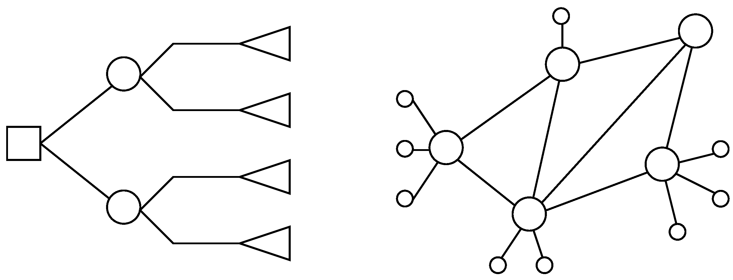
Those topologies have been divided into tree-like designs and graph-like designs, where in the former, nodes are interconnected through a hierarchy of switches, whereas in the latter, such interconnections are made directly between pairs of nodes.

The arithmetic study has consisted in the definition of two parameters, those being the average number of hops among nodes and the average number of links among devices, and in turn, a coefficient called $\eta$ has been defined as the product of both in order to provide a balance between both parameters.

On the one hand, the first parameter is related to performance, as the lower number of hops among nodes, the better, whilst on the other hand, the second parameter is related to simplicity, as the lower number of links per device, the better.

After having tested those parameters in different topologies mainly focused onsmall data centers, where the number of nodes is small to middle sized, it appears thatin tree-like designs, the value of coefficient $\eta$ grows as the average number of hops among nodes increases, even though the average number of links per device decreases at the same time. Otherwise, it seems thatin graph-like designs, the value of coefficient $\eta$ rises as the average number of links per device increases, although the average number of hops decreases at the same time.

Furthermore, some of the most commonly used network topologies in large data centers have also been studied, leading to coherent results obtained by coefficient $\eta$, which implies that this coefficient may be employed in data center networks of any size.

References

1. Pérez, J.; Díaz, J.; Berrocal, J.; López-Viana, R.; González-Prieto, A. Edge Computing. Computing 2022, 104, 2711–2747. [Google Scholar] [CrossRef]
2. Cao, K.; Liu, Y.; Meng, G.; Sun, Q. An Overview on Edge Computing Research. IEEE Access 2020, 8, 85714–85728. [Google Scholar] [CrossRef]
3. Filali, A.; Abouaomar, A.; Cherkaoui, S.; Kabbane, A.; Guizani, M. Multi-Access Edge Computing: A Survey. IEEE Access 2020, 8, 197017–197046. [Google Scholar] [CrossRef]
4. Ali, B.; Gregory, M.A.; Li, S. Multi-Access Edge Computing Architecture, Data Security and Privacy: A Review. IEEE Access 2021, 9, 18706–18721. [Google Scholar] [CrossRef]
5. Chen, S.; Jiao, L.; Liu, F.; Wang, L. EdgeDR: An Online Mechanism Design for Demand Response in Edge Clouds. IEEE Trans. Parallel Distrib. Syst. 2022, 33, 343–358. [Google Scholar] [CrossRef]
6. Girolami, M.; Vitello, P.; Capponi, A.; Fiandrino, C.; Foschini, L.; Bellavista, P. A mobility-based deployment strategy for edge data centers. J. Parallel Distrib. Comput. 2022, 164, 133–141. [Google Scholar] [CrossRef]
7. Liu, J.; Zhang, F.; Li, H.; Wang, D.; Wan, W.; Fang, X.; Zhai, J.; Du, X. Exploring Query Processing on CPU-GPU Integrated Edge Device. IEEE Trans. Parallel Distrib. Syst. 2022, 33, 4057–4070. [Google Scholar] [CrossRef]
8. Aravanis, A.I.; Voulkidis, A.; Salom, J.; Townley, J.; Georgiadou, V.; Oleksiak, A.; Porto, M.R.; Roudet, F.; Zahariadis, T. Metrics for Assessing Flexibility and Sustainability of Next Generation Data Centers. In Proceedings of the IEEE Globecom Workshops (GC Wkshps 2015), San Diego, CA, USA, 6–10 December 2015. [Google Scholar]
9. Román, R.; López, J.; Mambo, M. Mobile Edge Computing, Fog et al.: A Survey and Analysis of Security Threats and Challenges. Future Gener. Comput. Syst. 2018, 78, 680–698. [Google Scholar] [CrossRef] [Green Version]
10. Abreha, H.G.; Hayajneh, M.; Serhani, M.A. Federated Learning in Edge Computing: A Systematic Survey. Sensors 2022, 22, 450. [Google Scholar] [CrossRef]
11. Dimolitsas, I.; Dechouniotis, D.; Papavassiliou, S.; Papadimitriou, P.; Theodorou, V. Edge Cloud Selection: The Essential Step for Network Service Marketplaces. IEEE Commun. Mag. 2021, 59, 28–33. [Google Scholar] [CrossRef]
12. Liu, B.; Meng, S.; Jiang, X.; Xu, X.; Qi, L.; Dou, W. A QoS-guaranteed online user data deployment method in edge cloud computing environment. J. Syst. Archit. 2021, 118, 102185. [Google Scholar] [CrossRef]
13. Toczé, K.; Madon, M.; García, M.; Lago, P. The Dark Side of Cloud and Edge Computing: An Exploratory Study. In Proceedings of the 8th Workshop on Computing within Limits, Virtual Event, 21–22 June 2022. [Google Scholar]
14. Bellamy, L.A.; Henning, T.F.P.; Amor, R.; Jones, D.; Pancholy, P.; Preston, G.; van Jakobus, E. Data strategies for improving infrastructure value and performance in New Zealand. Proc. Inst. Civ.-Eng.–Smart Infrastruct. Constr. 2022, 2200008. [Google Scholar] [CrossRef]
15. Golightly, L.; Chang, V.; Xu, Q.A.; Gao, X.; Liu, B.S. Adoption of cloud computing as innovation in the organization. Int. J. Eng. Bus. Manag. 2022, 14. [Google Scholar] [CrossRef]
16. Andrae, A.S.G.; Edler, T. On Global Electricity Usage of Communication Technology: Trends to 2030. Challenges 2015, 6, 117–157. [Google Scholar] [CrossRef] [Green Version]
17. Manganelli, M.; Soldati, A.; Martirano, L.; Ramakrishna, S. Strategies for Improving the Sustainability of Data Centers via Energy Mix, Energy Conservation, and Circular Energy. Sustainability 2021, 13, 6114. [Google Scholar] [CrossRef]
18. Emara, T.Z.; Huang, J.Z. Distributed Data Strategies to Support Large-Scale Data Analysis Across Geo-Distributed Data Centers. IEEE Access 2020, 8, 178526–178538. [Google Scholar] [CrossRef]
19. Mansouri, N.; Javidi, M.M.; Zade, B.M.H. Hierarchical data replication strategy to improve performance in cloud computing. Front. Comput. Sci. 2021, 15, 152501. [Google Scholar] [CrossRef]
20. Ruan, L.; Xu, X.; Xiao, L.; Ren, L.; Min-Allah, N.; Xue, Y. Evaluating performance variations cross cloud data centres using multiview comparative workload traces analysis. Connect. Sci. 2022, 34, 1. [Google Scholar] [CrossRef]
21. Zhang, Y.; Liu, J. Prediction of Overall Energy Consumption of Data Centers in Different Locations. Sensors 2022, 22, 3704. [Google Scholar] [CrossRef]
22. Wang, T.; Su, Z.; Xiz, Y.; Hamdi, M. Rethinking the Data Center Networking: Architecture, Network Protocols, and Resource Sharing. IEEE Access 2014, 2, 1481–1496. [Google Scholar] [CrossRef]
23. Hoefler, T.; Hendel, A.; Roweth, D. The Convergence of Hyperscale Data Center and High-Performance Computing Networks. Computer 2022, 55, 29–37. [Google Scholar] [CrossRef]
24. Shen, L.; Qian, S.; Zhai, T.; Li, L.; Li, Z. Research on cloud computing high-density data center infrastructure and environment matching technology. MATEC Web Conf. 2021, 336, 02028. [Google Scholar] [CrossRef]
25. Wang, X.; Fan, J.X.; Lin, C.K.; Zhou, L.Y.; Liu, Z. BCDC: A High-Performance, Server-Centric Data Center Network. J. Comput. Sci. Technol. 2018, 33, 400–416. [Google Scholar] [CrossRef]
26. Raiciu, C.; Barre, S.; Pluntke, C.; Greenhalgh, A.; Wischik, W.; Handley, M. Improving datacenter performance and robustness with multipath TCP. Acm Sigcomm Comput. Commun. Rev. 2011, 41, 266–277. [Google Scholar] [CrossRef]
27. Cho, J.; Kim, Y. Development of modular air containment system: Thermal performance optimization of row-based cooling for high-density data centers. Energy 2021, 231, 120838. [Google Scholar] [CrossRef]
28. Patra, S.S.; Goswami, V. Performance Enhancement of Cloud Datacenters Through Replicated Database Server. J. Inf. Technol. Res. 2022, 15, 48. [Google Scholar] [CrossRef]
29. Cui, Y.; Jin, S.; Yue, W.; Takahashi, Y. Performance Optimization of Cloud Data Centers with a Dynamic Energy-Efficient Resource Management Scheme. Complexity 2021, 2021, 6646881. [Google Scholar] [CrossRef]
30. Feng, A.; Dong, D.; Lei, F.; Ma, J.; Yu, E.; Wang, R. In-network aggregation for data center networks: A survey. Comput. Commun. 2023, 198, 63–76. [Google Scholar] [CrossRef]
31. Almasan, P.; Xiao, S.; Cheng, X.; Shi, X.; Barlet-Ros, P.; Cabellos-Aparicio, A. ENERO: Efficient real-time WAN routing optimization with Deep Reinforcement Learning. Comput. Networks 2022, 214, 109166. [Google Scholar] [CrossRef]
32. Cao, B.; Zhao, J.; Yang, P.; Gu, Y.; Muhammad, K.; Rodrigues, J.J.; Alburquerque, V.H. Multiobjective 3-D Topology Optimization of Next-Generation Wireless Data Center Network. IEEE Trans. Ind. Inform. 2019, 1, 3597–3605. [Google Scholar] [CrossRef]
33. Roig, P.J. Formal Algebraic Modelling of a Fog Computer Network Architecture. Ph.D. Thesis, University of the Balearic Islands, Palma, Spain, 2022. [Google Scholar]
34. Hemachandra, K.G.R.P.; Jayasena, K.P.N.; Rankothge, W.; Wijesiri, M.P.M. Investigating the Performance in SDN Based Data Centers Under Different Network Topologies. In Proceedings of the 2nd International Conference on Advanced Research in Computing (ICARC), Belihuloya, Sri Lanka, 23–24 February 2022; pp. 361–366. [Google Scholar]
35. Bermejo, B. Performance and Energy Consumption Trade-Off in Server Consolidation. Ph.D. Thesis, University of the Balearic Islands, Palma, Spain, 2020. [Google Scholar]
36. Roig, P.J.; Alcaraz, S.; Gilly, K.; Bernad, C.; Juiz, C. Arithmetic Framework to Optimize Packet Forwarding among End Devices in Generic Edge Computing Environments. Sensors 2022, 22, 421. [Google Scholar] [CrossRef]
37. Deng, S.; Zhao, H.; Fang, W.; Yin, J.; Dustdar, S.; Zomaya, A.Y. Edge Intelligence: The Confluence of Edge Computing and Artificial Intelligence. IEEE Internet Things J. 2020, 7, 7457–7469. [Google Scholar] [CrossRef] [Green Version]
38. Kubler, S.; Rondeau, E.; Georges, J.P.; Mutua, P.L.; Chinnici, M. Benefit-cost model for comparing data center performance from a biomimicry perspective. J. Clear Prod. 2019, 231, 817–834. [Google Scholar] [CrossRef]
39. Al-Fares, M.; Loukissas, A.; Vahdat, A. A Scalable, Commodity Data Center Network Architecture. ACM SIGCOMM Comput. Commun. Rev. 2008, 38, 63–74. [Google Scholar] [CrossRef] [Green Version]
40. Okafor, K.C.; Achumba, I.E.; Chukwudebe, G.A.; Ononiwu, G.C. Leveraging Fog Computing for scalable IoT datacenter using Spine-Leaf network topology. J. Electr. Comput. Eng. 2017, 2017, 2363240. [Google Scholar] [CrossRef] [Green Version]
41. Correia, I.; Nickel, S.; Saldanha-da-Gama, F. Hub and spoke network design with single-assignment, capacity decisions and balancing requirements. Appl. Math. Model. 2011, 35, 4841–4851. [Google Scholar] [CrossRef]
42. Guo, C.; Lu, G.; Li, D.; Wu, H.; Zhang, X.; Shi, Y.; Tian, C.; Zhang, Y.; Lu, S. BCube: A High Performance, Server-centric Network Architecture for Modular Data Centers. In Proceedings of the SIGCOMM 2009, Barcelona, Spain, 17–21 August 2009. [Google Scholar]
43. Guo, C.; Wu, H.; Tan, K.M.; Shi, L.; Zhang, Y.; Lu, S. DCell: A Scalable and Fault-Tolerant Network Structure for Data Centers. In Proceedings of the SIGCOMM 2008, Seattle, WA, USA, 17–22 August 2008. [Google Scholar]
44. Li, D.; Guo, C.; Wu, H.; Tan, K.; Zhang, Y.; Lu, S. FiConn: Using Backup Port for Server Interconnection in Data Centers. In Proceedings of the INFOCOM 2009, Rio de Janeiro, Brazil, 19–25 April 2009; pp. 2276–2285. [Google Scholar]
45. Kim, J.; Balfour, J.; Dally, W.J. Flattened Butterfly Topology for On-Chip Networks. In Proceedings of the 40th Annual IEEE/ACM International Symposium on Microarchitecture (MICRO 2007), Chicago, IL, USA, 1–5 December 2007; pp. 172–182. [Google Scholar]
46. Kim, J.; Dally, W.J.; Scott, S.; Abts, D. Technology-Driven, Highly-Scalable Dragonfly Topology. In Proceedings of the International Symposium on Computer Architecture (ISCA 2008), Beijing, China, 21–25 June 2008; pp. 77–88. [Google Scholar]
47. Besta, M.; Hoefler, T. Slim Fly: A Cost Effective Low-Diameter Network Topology. In Proceedings of the International Conference for High Performance Computing, Networking, Storage and Analysis (SC 2014), New Orleans, LA, USA, 16–21 November 2014; pp. 348–359. [Google Scholar]
48. Slim Fly: A Cost Effective Low-Diameter Network Topology. Available online: https://spcl.inf.ethz.ch/Research/Scalable_Networking/SlimFly/ (accessed on 7 January 2023).
49. Kan, S.; Fan, J.; Cheng, B.; Wang, X. The Communication Performance of BCDC Data Center Network. In Proceedings of the 2th International Conference on Communication Software and Networks (ICCSN), Chongqing, China, 12–15 June 2020; pp. 51–57. [Google Scholar]
50. Dash, R.K. A New Cost Effective and Reliable Interconnection Topology for Parallel Computing Systems. Int. J. Eng. Adv. Technol. 2019, 8, 1186–1195. [Google Scholar]
51. Qin, X.W.; Hao, R.X. Hamiltonian properties of some compound networks. Discret. Appl. Math. 2018, 239, 174–182. [Google Scholar] [CrossRef]
52. ALzaid, Z.; Bhowmik, S.; Yuan, X. Multi-Path Routing on the Jellyfish Networks. In Proceedings of the IEEE International Parallel and Distributed Processing Symposium Workshops (IPDPSW), Portland, OR, USA, 17 May 2021; pp. 832–841. [Google Scholar]
53. Singla, A.; Hong, C.Y.; Popa, L.; Godfrey, P.B. Jellyfish: Networking Data Centers Randomly. In Proceedings of the 9th USENIX conference on Networked Systems Design and Implementation (NSDI 2012), San Jose, CA, USA, 25–27 April 2012. [Google Scholar]
54. Liu, V.; Zhuo, D.; Peter, S.; Krishnamurthy, A.; Anderson, T. Subways: A Case for Redundant, Inexpensive Data Center Edge Links. In Proceedings of the 11th ACM Conference on Emerging Networking Experiments and Technologies (CoNEXT 2015), Heidelberg, Germany, 1–4 December 2015. [Google Scholar]
55. Rezaei, H.; Vamanan, B. Jellyfish: Superways: A Datacenter Topology for Incast-heavy workloads. In Proceedings of the Web Conference 2021 (WWW 2021), Ljubljana, Slovenia, 19–23 April 2021. [Google Scholar]
56. Couto, R.S.; Secci, S.; Campista, M.E.M.; Costa, L.H.M. Reliability and Survivability Analysis of Data Center Network Topologies. J. Netw. Syst. Manag. 2016, 24, 346–392. [Google Scholar] [CrossRef] [Green Version]
57. Negara, E.S.; Keni, K.; Andryani, R. BCube and DCell Topology Data Center Infrastructures Performance. IOP Conf. Ser. Mater. Sci. Eng. 2020, 852, 012129. [Google Scholar] [CrossRef]
58. Cortés-Castillo, A. Various Network Topologies and an Analysis Comparative Between Fat-Tree and BCube for a Data Center Network: An Overview. In Proceedings of the IEEE Cloud Summit, Fairfax, VA, USA, 20–21 October 2022. [Google Scholar]
59. Al-Makhlafi, M.; Gu, H.; Yu, X.; Lu, Y. P-Cube: A New Two-Layer Topology for Data Center Networks Exploiting Dual-Port Servers. IEICE Trans. Commun. 2020, 103, 940–950. [Google Scholar] [CrossRef]
60. Liu, Y.; Gao, X.; Chen, G. Design and Optimization for Distributed Indexing Scheme in Switch-Centric Cloud Storage System. In Proceedings of the 20th IEEE Symposium on Computers and Communication (ISCC), Larnaca, Cyprus, 6–9 July 2015. [Google Scholar]
61. Yao, F.; Wu, J.; Venkataramani, G.; Subramaniam, S. A Comparative Analysis of Data Center Network Architectures. In Proceedings of the IEEE International Conference on Communications (ICC), Sidney, Australia, 10–14 June 2014; pp. 3106–3111. [Google Scholar]
62. Touihri, R.; Alwan, S.; Dandoush, A.; Aitsaadi, N.; Veillon, C. CRP: Optimized SDN Routing Protocol in Server-Only CamCube Data-Center Networks. In Proceedings of the 2019 IEEE International Conference on Communications (ICC), Shanghai, China, 20–24 May 2019. [Google Scholar]
63. Daryin, A.; Korzh, A. Early evaluation of direct large-scale InfiniBand networks with adaptive routing. Supercomput. Front. Innov. 2014, 1, 56–69. [Google Scholar]
64. Rao, M.V.; Krishna, T.V.R.; Sruthi, S.R.S.; Akhila, S.; Gopi, Y.; Krishna, L.B. An Effective on-Chip Network Topology for Network on Chip (Noc) Trade-Offs. Indian J. Sci. Technol. 2016, 9, 17. [Google Scholar]
65. Azizi, S.; Hashemi, N.; Khonsari, A. A flexible and high-performance data center network topology. J. Supercomput. 2017, 73, 1484–1503. [Google Scholar] [CrossRef]
66. Aguirre-Guerrero, D.; Camelo, M.; Fàbrega, L.; Vilà, P. WMGR: A Generic and Compact Routing Scheme for Data Center Networks. IEEE/ACM Trans. Netw. 2018, 26, 356–369. [Google Scholar] [CrossRef]
67. Mohamed, S.H.; El-Gorashi, T.E.H.; Elmirghani, J.M.H. Energy Efficiency of Server-Centric PON Data Center Architecture for Fog Computing. In Proceedings of the 20th International Conference on Transparent Optical Networks (ICTON), Bucharest, Romania, 1–5 July 2018. [Google Scholar]
68. Sego, L.H.; Márquez, A.; Rawson, A.; Cader, T.; Fox, K.; Gustafson, W.I.; Mundy, C.J. Implementing the data center energy productivity metric. ACM J. Emerg. Technol. Comput. Syst. 2012, 8, 030. [Google Scholar] [CrossRef]
69. Santos, A.F.; Gaspar, P.D.; de Souza, H.J.L. New Data Center Performance Index: Perfect Design Data Center—PDD. Climate 2020, 8, 110. [Google Scholar] [CrossRef]
70. Shao, X.; Zhang, Z.; Song, P.; Feng, Y.; Wang, X. A review of energy efficiency evaluation metrics for data centers. Energy Build. 2022, 271, 112308. [Google Scholar] [CrossRef]
71. Levy, M.; Raviv, D. A Novel Framework for Data Center Metrics using a Multidimensional Approach. In Proceedings of the 15th LACCEI International Multi-Conference for Engineering, Education, and Technology: Global Partnerships for Development and Engineering Educatio, Boca Ratón, FL, USA, 19–21 July 2017. [Google Scholar]
72. Kumar, R.; Khatri, S.K.; Diván, M.J. Performance Analysis of Machine Learning Regression Techniques to Predict Data Center Power Usage Efficiency. Int. J. Eng. Trends Technol. 2022, 70, 328–338. [Google Scholar] [CrossRef]
73. Brocklehurs, F. International Review of Energy Efficiency in Data Centres for IEA EBC Building Energy Codes Working Group. Available online: https://www.iea-ebc.org/Data/publications/EBC_WG_BECs_Data_Centers_March_2022.pdf (accessed on 30 May 2023).
74. Reddy, V.D.; Setz, B.; Rao, G.S.V.; Gangadharan, G.R.; Aiello, M. Metrics for Sustainable Data Centers. IEEE Trans. Sustain. Comput. 2017, 2, 290–303. [Google Scholar] [CrossRef] [Green Version]
Figure 1. Tree-like design (left) -vs.- graph-like design (right).
Network 03 00015 g001
Figure 2. Devices in each layer in a fat tree topologywith k = 4 and oversubscription rate 1:1.
Network 03 00015 g002
Figure 3. Devices in each layer in a leaf and spine topologywith 8 leaves and 4 spines.
Network 03 00015 g003
Figure 4. Devices in each layer in a redundant hub and spoke topologywith 6 spokes and a single hub (left) or a redundant hub (right).
Network 03 00015 g004
Figure 5. Nodes in N-hypercubes of dimensions { 0 4 } (from left to right).
Network 03 00015 g005
Figure 6. Nodes in folded N-hypercubes of dimensions { 2 4 } (from left to right).
Network 03 00015 g006
Figure 7. Nodes in N-simplices of dimensions { 1 4 } (from left to right).
Network 03 00015 g007
Figure 8. Nodes in N-orthoplices of dimensions { 1 4 } (from left to right).
Network 03 00015 g008
Figure 9. Nodes in k-ary n-cube (left: 4-ary 1-cube; right: 4-ary 2-cube).
Network 03 00015 g009
Figure 10. Nodes in Hamming graph H ( n , n 1 ) (left: n = 2 ; right: n = 4 ).
Network 03 00015 g010
Figure 11. Nodes in Petersen graph, a ( 3 , 5 ) -cage with 10 nodes.
Network 03 00015 g011
Figure 12. Nodes in Heawood graph, a ( 3 , 6 ) -cage with 14 nodes.
Network 03 00015 g012
Figure 13. Nodes in Robertson graph, a ( 4 , 5 ) -cage with 19 nodes.
Network 03 00015 g013
Figure 14. Nodes in a BCube 1 topology with n = 4 .
Network 03 00015 g014
Figure 15. Nodes in a DCell 1 topology with n = 4 .
Network 03 00015 g015
Figure 16. Nodes in FiConn 2 topology with n = 4 .
Network 03 00015 g016
Figure 17. Nodes in a Flattened Butterfly topology with n = 4 (left) and n = 3 (right).
Network 03 00015 g017
Figure 18. Nodes in a DragonFly topology with g = 9 and a = 4 .
Network 03 00015 g018
Figure 19. Nodes in a SlimFly topology, with groups of 5 routers forming a fully connected bipartite graph of diameter 2.
Network 03 00015 g019
Figure 20. Nodes in a BCDC topology in 3 dimensions.
Network 03 00015 g020
Figure 21. Nodes in a P-Cube topology with n = 4 .
Network 03 00015 g021
Figure 22. Nodes in a DCCube topology with k = 1 , m = 4 , h = 1 and c = 2 .
Network 03 00015 g022
Figure 23. Nodes in a Jellyfish topology with N = 15 , x = 4 and y = 3 .
Network 03 00015 g023
Figure 24. Nodes in a Subway topology with p = 3 and l = 3 .
Network 03 00015 g024
Figure 25. Nodes in a Superways topology with L = 2 .
Network 03 00015 g025
Figure 26. Coefficient for topologies with 2 nodes.
Network 03 00015 g026
Figure 27. Coefficient for topologies with 4 nodes.
Network 03 00015 g027
Figure 28. Coefficient for topologies with 8 nodes.
Network 03 00015 g028
Figure 29. Coefficient for topologies with 16 nodes.
Network 03 00015 g029
Figure 30. Coefficient for small topologies not being a power of 2.
Network 03 00015 g030
Figure 31. Coefficient for topologies commonly used in data centers.
Network 03 00015 g031
Figure 32. Coefficient for topologies with many nodes.
Network 03 00015 g032