1. Introduction
Many petroleum derivatives are used as lubricants, essential for the correct functioning of some equipment that depends on the appropriate viscosity of the fluid used. Therefore, the viscosity of these petroleum fuels is important for estimating ideal storage, handling, and operating conditions. Therefore, reliable viscosity determination is essential for many product specifications [
1].
Kinematic viscosity is the relationship between momentum transport and momentum storage. Such relationships are called diffusivities, with dimensions of length squared divided by time, and the SI unit is a square metre divided per second (m2/s). However, in the oil and gas industry, it is normally converted to cSt (1 mm2/s = 10−6 m2/s = 1 cSt). Among the transport properties for heat, mass, and momentum transfer, kinematic viscosity is momentum diffusivity.
The literature presents some studies concerning the kinematic viscosity determined with ASTM D445 [
1], such as the investigation of the difference in vehicle engine performance due to degradation of engine oil properties [
2]; the kinematic viscosity of engine oils is reduced by the influence of the accumulation of gasoline–bioethanol mixtures [
3]; the characterisation of used oil distillate [
4]; and the investigation of kinematic viscosity and other physicochemical properties arising from storage in biodiesel mixtures derived from used cooking oils [
5]. Few studies shed light on the kinematic viscosity of opaque liquids determined using ASTM D445 [
6,
7,
8]. Recently and in a still timid manner, some studies using the design of experiments have been applied to fuel and biofuels, such as the prediction of the physical properties of biofuels [
9], the evaluation of the correlation between the ratio of light biofuel and refined palm oil blends on their density and kinematic viscosity properties [
10], and the minimisation of the kinematic viscosity and maximisation of the biodiesel yield during a transesterification reaction [
11]. Furthermore, kinematic viscosity has been used in several studies regarding the quality of biodiesel [
12,
13,
14,
15].
The analytical procedure for testing residual fuel oils and opaque liquids recommends heating the sample in the original container at 60 °C and 65 °C for 1 h, unlike the procedure for transparent liquids [
1].
Uniform heating time for opaque oils may be important; however, from a physical point of view, if there are no chemical transformations in the liquid or no dissolution process, the heating rate does not affect the physicochemical properties. On the other hand, the purpose of warming up the product before testing is to facilitate its pouring into the viscometer tube and the dissolution of paraffins, if present.
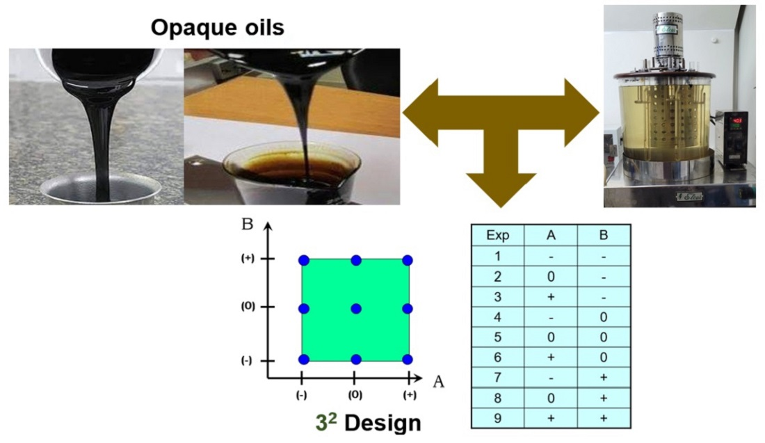
Therefore, this study aimed to evaluate metrologically, through the design of experiments, whether there are significant differences in the kinematic viscosity results, specifically of very low sulphur fuel oil (VLSFO), Brazilian fuel oil, and atmospheric residue diluted with diesel oil (RAT), which are fluids at room temperature, when they receive the same treatment as transparent liquids; that is, they are not heated.
2. Design of Experiments
Many experiments aim to evaluate the effects and possible correlations of two or more factors. Whenever it is necessary to reduce the number of experiments and increase the maximum amount of information about the system, factorial designs are recommended, as they are more efficient and effective. When using a factorial design, all possible combinations of factor levels are examined in each complete trial or replication of the experiment. For instance, for levels a of factor A and b of factor B, in addition to information regarding their own levels, it is possible to have information about combinations ab, which are normally called interactions.
Variations in the response (output magnitude) can be observed when each factor (input quantity) passes from one level to another, which can be defined as the effect of the factor. When this effect refers to the main factors of interest in the experiment, it is called the main effect. The simplest case is a two-factor factorial experiment with both design factors at two levels. The low level is also called “−1”, while the high level is named “+1”. The main effect of factor A in a two-level design can be understood as the difference perceived in the average output quantity when going from the low level to the high level of
A [
16].
The simplest case is a factorial design with two factors. To move on to the general case, let
yijk be the response observed when factor
A is at the
i-th level (
i = 1, 2, ...,
a) and factor
B is at the
j-th level (
j = 1, 2, ...,
b) for the
k-th replica (
k = 1, 2, ...,
n). In general, a two-factorial design will appear as in
Table 1. To guarantee randomness to the process,
abn observations are performed in a completely random sequence.
,
, and
define the total of all observations related to the
ith level of factor
A, the
jth level of the factor
B, and its grand total, respectively. And their respective averages can be calculated as follows:
| | i = 1, 2, ..., a | rows |
| | j = 1, 2, ..., b | columns |
| | i = 1, 2, ..., a
j = 1, 2, ..., b | cells |
| | | grand |
Finally, the corrected total sum of squares is written as
The total sum of squares has been spread over a sum of squares due to the “rows”, or factor A (SSA); a sum of squares due to “columns”, or factor B (SSB); a sum of squares related to the interaction between A and B (SSAB); and a sum of squares concerning the residual or error (SSE). This information is available in algorithms for two-way ANOVA with interaction.
Presuming that the data are normally homoscedastic and independently distributed, the relationship between variances, mean squares, and their respective degrees of freedom can be used to evaluate the relevance of each parameter (
Table 2).
3. Material and Methods
In this section, the products and test method used are described.
3.1. Experimental
The study, relating to samples using VLSFO (very low sulphur fuel oil), fuel oil (OCA1), and atmospheric residue diluted with diesel oil (RAT) (
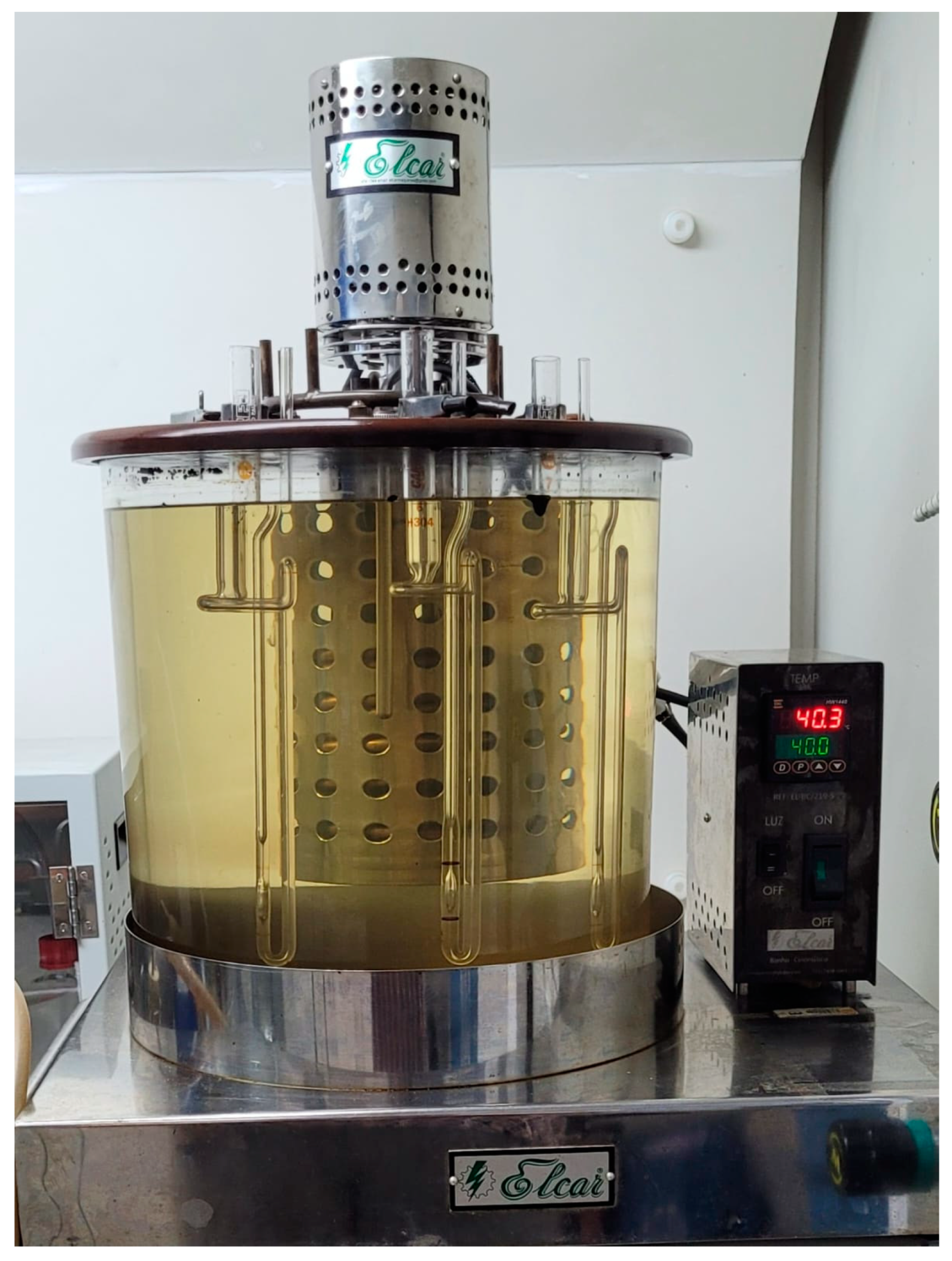
Table 3), was carried out in August 2022 in a Brazilian fuel storage terminal without heating, with heating between 60 °C and 65 °C for 30 min, and heating between 60 °C and 65 °C for 60 min. The viscometers used were the routine Cannon–Fenske reverse-flow type.
The glass capillary viscometers, the temperature measuring, and the timing devices,
Figure 1, were calibrated within their expiration dates.
In a simplified way, the procedure used for determining the kinematic viscosity of these opaque oils was as follows: (i) we charged the reverse-flow-type viscometer with the opaque oils; (ii) we placed the viscometer in the viscometer bath at the desired test temperature; (iii) we let the charged viscometer remain in the bath for enough time to reach the test temperature; and (iv) after ensuring that the opaque oil flowed freely, we measured to the nearest 0.1 s the time required for the sample to flow between the calibrated marks on the viscosimetric tube.
At least two kinematic viscosity determinations are necessary to consider a valid result. The test results for the kinematic viscosity were reported in four significant figures.
3.2. Test Method
The test method details an experimental procedure for evaluating the kinematic viscosity of opaque and transparent liquid petroleum products. The analytical principle is based on measuring the time it takes a portion of the sample to flow under gravity using a calibrated glass capillary viscometer [
1].
The time is measured for a constant volume of liquid to flow under gravity through the capillary of a calibrated viscometer under a reproducible drive head and at a known, tightly controlled temperature. The kinematic viscosity (determined value) is the product of the measured flow time and the viscometer calibration constant. Two such determinations are required to calculate a kinematic viscosity result, i.e., the average of two acceptable determined values.
4. Results and Discussion
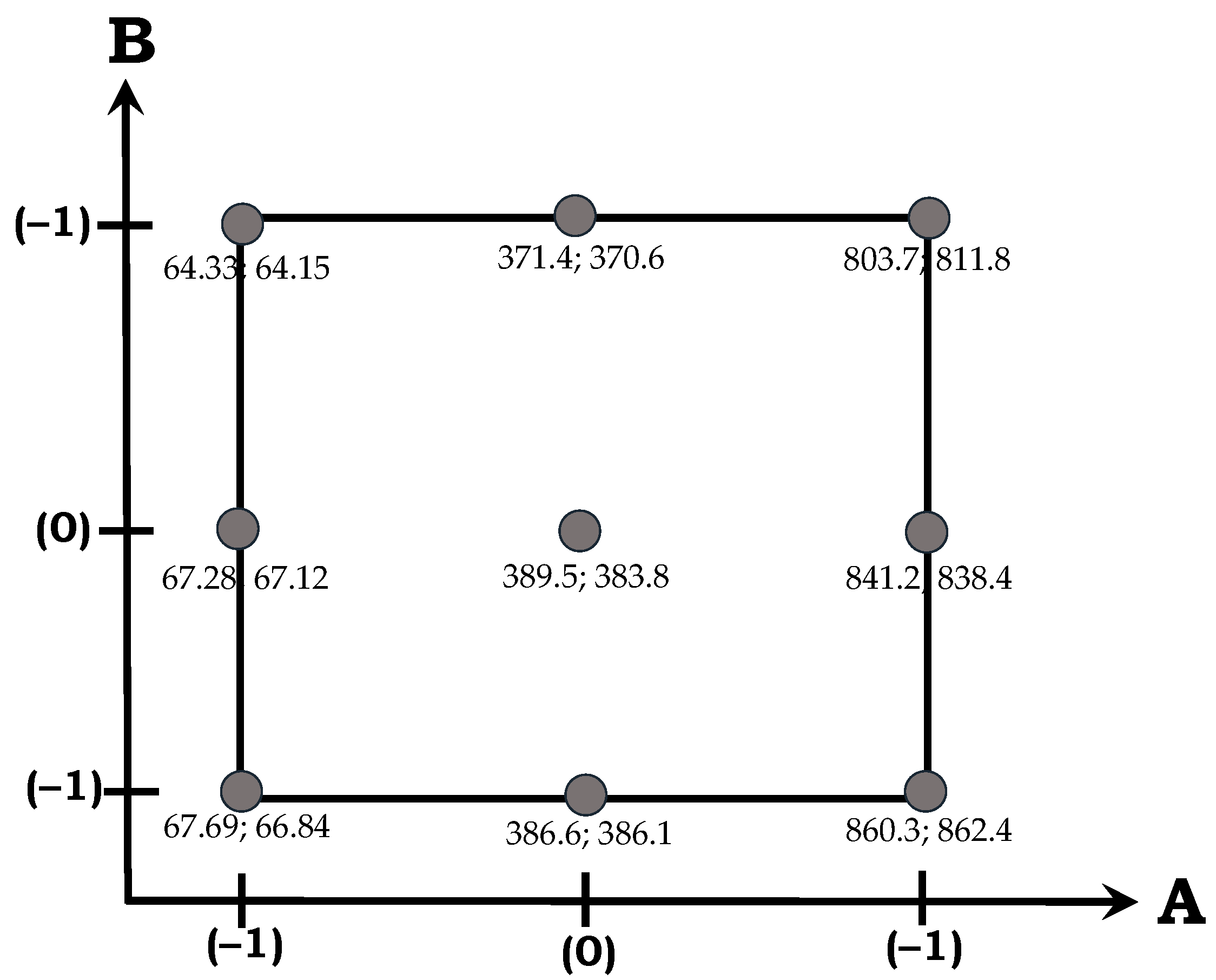
The matrix,
, with the experiment and design—considering two factors and three levels—is detailed in
Table 4.
A is the product and B is the warm-up time, with two replicates of the output quantity, kinematic viscosity, R1, and R2. The graphical representation of the matrix
is shown in
Figure 2.
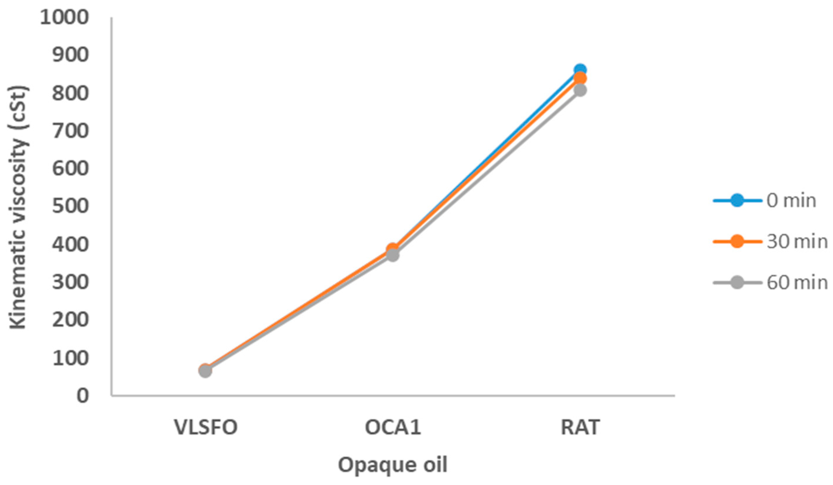
To help interpret the results of this experiment, it is useful to plot the average responses for each treatment combination in
Figure 3.
The absence of significant interaction is indicated by the parallelism of the lines. Visually, the kinematic viscosity is not significantly affected by the warm-up time.
The contrasts—linear combination of parameters; effects, change suffered by the response variable when moving from the low level of the factor to the highest level; coefficients (and their standard errors); and the sum of squares (SS)—were calculated considering an
of 1418.615 (
Table 2).
For factor
B (warm-up time),
For the interaction between factors
A and
B,
The
. Considering 3 degrees of freedom (df), the
is
. For evaluating the efficiency of the regression,
Fcalculated was
, greater than
Fcritical (0.05; 3; 14) = 3.34, which warranted that this regression was significant [
17].
These data were subjected to a two-way ANOVA with interaction (
Table 5).
Firstly, the relevance of each regression coefficient was evaluated based on the F test [
17]:
;
; and
. Comparing the
Fcritical (0.05; 1; 14) = 4.600 with these
Fcalculated, one concluded that only factor A (product) significantly impacted on the kinematic viscosity output quantity.
Based on the
p-value, factor A, the product has significantly impacted the kinematic viscosity output quantity since the
p-value was less than 5% [
18,
19]. However, factor B, warm-up time, did not significantly impact the kinematic viscosity output quantity since the
p-value is greater than 5%. A lack of interaction between the product and warm-up time variables can also be observed.
A third approach used the confidence intervals (CI) of the regression coefficients, which were calculated as follows:
[
20].
; ; and . One only considers statistically significant effects whose estimates (obtained in the experiment) are greater in absolute value than the product of the standard error and critical values of the Student’s t-distribution because, this way, the confidence interval does not include the zero value. Thus, only factor A proved relevant, confirming the two previous approaches.
Lastly, using the percentage contribution of the sum of squares approach [
17], the relevance of each factor was evaluated as follows:
;
; and
. The warm-up time and its interaction with the product did not have a significant impact on the kinematic viscosity output quantity since their percentages were less than 5%.
5. Conclusions
A statistical design of experiments was used to plan the experiment so that appropriate data could be collected and analysed using metrological approaches such as regression analysis and ANOVA. Here, the minimum number of experiments was carried out, and the maximum information regarding this measurement system was achieved.
This study evaluated metrologically, through experimental design and four different approaches, that there were no significant differences in the kinematic viscosity results of VLSFO, OCA1, and RAT when they were not heated for 1 h to a temperature between 60 °C and 65 °C.
Author Contributions
Conceptualisation, M.A.C.d.C., G.K.B.M. and E.C.d.O.; methodology, M.A.C.d.C., G.K.B.M. and E.C.d.O.; software, M.A.C.d.C., G.K.B.M. and E.C.d.O.; validation, M.A.C.d.C., G.K.B.M. and E.C.d.O.; formal analysis, M.A.C.d.C., G.K.B.M. and E.C.d.O.; investigation, M.A.C.d.C., G.K.B.M. and E.C.d.O.; resources, M.A.C.d.C., G.K.B.M. and E.C.d.O.; data curation, M.A.C.d.C., G.K.B.M. and E.C.d.O.; writing—original draft preparation, M.A.C.d.C., G.K.B.M. and E.C.d.O.; writing—review and editing, M.A.C.d.C., G.K.B.M. and E.C.d.O.; visualisation, M.A.C.d.C., G.K.B.M. and E.C.d.O.; supervision, M.A.C.d.C., G.K.B.M. and E.C.d.O.; project administration, M.A.C.d.C., G.K.B.M. and E.C.d.O.; funding acquisition, M.A.C.d.C., G.K.B.M. and E.C.d.O. All authors have read and agreed to the published version of the manuscript.
Funding
The authors thank the Brazilian agency CNPq for the financial support provided through the scholarship (305479/2021-0). This study was financed in part by the Coordenação de Aperfeiçoamento de Pessoal de Nível Superior—Brasil (CAPES)—Finance Code 001.
Institutional Review Board Statement
Not applicable.
Informed Consent Statement
Not applicable.
Data Availability Statement
Data are contained within the article.
Conflicts of Interest
The authors declare no conflicts of interest.
References
- ASTM D445-21; Standard Test Method for Kinematic Viscosity of Transparent and Opaque Liquids (and Calculation of Dynamic Viscosity). American Society for Testing and Materials: West Conshohocken, PA, USA, 2021.
- Hameed, D. Effects of Vehicle Mileage Rate on Engine Oil Properties. Passer J. Basic Appl. Sci. 2023, 5, 59–64. [Google Scholar] [CrossRef]
- Hanifuddin, M.; Malik, R.; Fibria, M.; Respatiningsih, C.Y.; Karina, R.M.; Widodo, S.; Purnami, T.; Anggarani, R.; Maymuchar; Wibowo, C.S. The Influence of Gasoline-Bioethanol Blends on Lubrication Characteristic of 4T Motorcycle Engine Oil. IOP Conf. Ser. Earth Environ. Sci. 2022, 1034, 012030. [Google Scholar] [CrossRef]
- Firman, M.; Arief, S.; Julianda, H.; Fauzan, M.; Saukani, M. Characterization of used oil distillate at various distillation temperatures as diesel fuel. IOP Conf. Ser. Earth Environ. Sci. 2021, 758, 012020. [Google Scholar] [CrossRef]
- Kassem, Y.; Çamur, H.; Alassi, E. Biodiesel Production from Four Residential Waste Frying Oils: Proposing Blends for Improving the Physicochemical Properties of Methyl Biodiesel. Energies 2020, 13, 4111. [Google Scholar] [CrossRef]
- Khuu, H.; Yee, N.; Butterfield, A.; Meiser, M.; Wei, T.; Gutsol, A.; Moir, M. Improving ASTMD445, the Manual Viscosity Test, by Video Recording. J. Test. Eval. 2019, 47, 310–323. [Google Scholar] [CrossRef]
- de Paula Pedroza, R.H.; Nicácio, J.T.N.; dos Santos, B.S.; de Lima, K.M.G. Determining the Kinematic Viscosity of Lubricant Oils for Gear Motors by Using the Near Infrared Spectroscopy (NIRS) and the Wavelength Selection. Anal. Lett. 2013, 46, 1145–1154. [Google Scholar] [CrossRef]
- Ghalehjooghi, A.S.; Minaei, S.; Zanjani, N.G.; Beheshti, B. Note: A portable automatic capillary viscometer for transparent and opaque liquids. Rev. Sci. Instrum. 2017, 88, 076108. [Google Scholar] [CrossRef] [PubMed]
- Wiseman, S.; Michelbach, C.A.; Li, H.; Tomlin, A.S. Predicting the physical properties of three-component lignocellulose derived advanced biofuel blends using a design of experiments approach. Sustain. Energy Fuels 2023, 7, 5283. [Google Scholar] [CrossRef]
- Mat, S.C.; Idroas, M.Y.; Teoh, Y.H.; Hamid, M.F. Optimisation of viscosity and density of refined palm Oil-Melaleuca Cajuputi oil binary blends using mixture design method. Renew. Energy 2019, 133, 393–400. [Google Scholar] [CrossRef]
- Gülüm, M.; Yesilyurt, M.K.; Bilgin, A. The modeling and analysis of transesterification reaction conditions in the selection of optimal biodiesel yield and viscosity. Environ. Sci. Pollut. Res. 2020, 27, 10351–10366. [Google Scholar] [CrossRef] [PubMed]
- Guimarães, C.C.; dos Santos, V.M.L.; Cortez, J.W.; dos Santos, L.P.G. Reduction emission of particulate matter as a function of insertion of biodiesel mixtures from soybean and castor bean in diesel. Eng. Sanit. Ambient. 2018, 23, 355–362. [Google Scholar] [CrossRef]
- Rathmann, R.; Szklo, A.; Schaeffer, R. Targets and results of the Brazilian Biodiesel Incentive Program—Has it reached the Promised Land? Appl. Energy 2012, 97, 91–100. [Google Scholar] [CrossRef]
- Chechetto, R.G.; Siqueira, R.; Gamero, C.A. Energy balance for biodiesel production by the castor bean crop (Ricinus communis L.). Ciênc. Agron. 2010, 41, 546–553. [Google Scholar] [CrossRef]
- Tabile, R.A.; Lopes, A.; Dabdoub, M.J.; da Camara, F.T.; Furlani, C.E.A.; da Silva, R.P. Mamona biodiesel in interior and metropolitan diesel in agricultural tractor. Eng. Agricola 2009, 29, 412–423. [Google Scholar] [CrossRef]
- Miller, J.N.; Miller, J.C.; Miller, R.D. Statistics and Chemometrics for Analytical Chemistry, 7th ed.; Coronet Books Inc.: London, UK, 2018. [Google Scholar]
- Montgomery, D.C. Design and Analysis of Experiments, 8th ed.; John Wiley & Sons, Inc.: Hoboken, NJ, USA, 2013. [Google Scholar]
- Guerra, M.J.P.; de Oliveira, E.C.; Frota, M.N.; Marques, R.P. Design of experiments for optimising acceptance calibration criteria for pressure and temperature transmitters of gas flowmeters. J. Nat. Gas Eng. 2018, 58, 26–33. [Google Scholar] [CrossRef]
- de Almeida, F.C.; de Oliveira, E.C.; Barbosa, C.R.H. Design of experiments to analyze the influence of water content and meter factor on the uncertainty of oil flow measurement with ultrasonic meters. Flow Meas. Instrum. 2019, 70, 101627. [Google Scholar] [CrossRef]
- De Barros Neto, B.; Scarminio, I.S.; Bruns, R.E. Como Fazer Experimentos, 4th ed.; Bookman, Ed.; Artmed Editora SA: Porto Alegre, Brazil, 2010; ISBN 978-85-7780-652-2. [Google Scholar]
| Disclaimer/Publisher’s Note: The statements, opinions and data contained in all publications are solely those of the individual author(s) and contributor(s) and not of MDPI and/or the editor(s). MDPI and/or the editor(s) disclaim responsibility for any injury to people or property resulting from any ideas, methods, instructions or products referred to in the content. |
© 2024 by the authors. Licensee MDPI, Basel, Switzerland. This article is an open access article distributed under the terms and conditions of the Creative Commons Attribution (CC BY) license (https://creativecommons.org/licenses/by/4.0/).


