A Possibilistic Kalman Filter for the Reduction of the Final Measurement Uncertainty, in Presence of Unknown Systematic Errors

Abstract

A Kalman filter is a concept that has been in existence for decades now and it is widely used in numerous areas. It provides a prediction of the system states as well as the uncertainty associated to it. The original Kalman filter can not propagate uncertainty in a correct way when the variables are not distributed normally or when there is a correlation in the measurements or when there is a systematic error in the measurements. For these reasons, there have been numerous variations of the original Kalman filter, most of them mathematically based (like the original one) on the theory of probability. Some of the variations indeed introduce some improvements, but without being completely successful. To deal with these problems, more recently, Kalman filters have also been defined using random-fuzzy variables (RFVs). These filters are capable of also propagating distributions that are not normal and propagating systematic contributions to uncertainty, thus providing the overall measurement uncertainty associated to the state predictions. In this paper, the authors make another step forward, by defining a possibilistic Kalman filter using random-fuzzy variables which not only considers and propagates both random and systematic contributions to uncertainty, but also reduces the overall uncertainty associated to the state predictions by compensating for the unknown residual systematic contributions.

1. Introduction

The Kalman filter (KF) is an algorithm that has long been in existence. It filters the noise on the measured values of the states and provides an estimation of the system states based on the state equations. The classical KF algorithm requires that the states are free from any systematic errors and that the state variables are independent from each other and can be represented by Gaussian distributions [1]. But in most practical situations, the systematic error can not be compensated perfectly and there is a residual systematic error. In this case, the classical formulations of the KF underestimate the uncertainty associated to the state estimates, because the systematic error is not propagated in a correct mathematical way. To deal with this, attempts have been made to develop KF algorithms that are also able to consider systematic contributions to uncertainty [2,3,4,5]. For instance, in [5], the authors try to use a Schmidt KF that considers the systematic error as a separate state in the state equations and a noise covariance matrix of the possible systematic errors is built and propagated.

More recently, the theory of possibility has been proposed in the literature to represent and propagate both systematic and random contributions to uncertainty. The theory of possibility has been proven by numerous applications in the literature [6,7,8,9,10,11] to be an effective alternative to the theory of probability when both random and systematic contributions to uncertainty are present in the measurement procedure.

Some attempts to define KFs based on the theory of possibility are already present in the literature [12,13]. However, in [12,13], as far as understood, they consider uncertainty in a fuzzy way that is not compatible with the recommended guidelines in metrology, as specified in [14,15]. In metrology, uncertainty must be considered according to the definitions given in [15].

Within the framework of the theory of possibility, quantities are represented by possibility distributions [16,17,18,19,20,21]. In particular, as shown in [16,17,18], where measurement results are considered to be affected by both random and systematic contributions to uncertainty, measured quantities are represented by random-fuzzy variables (RFVs). RFVs consist of an internal membership function which represents the systematic contribution to uncertainty in the quantity and an external membership function which represents the overall uncertainty due to both the systematic and random contributions. As shown in [16,18], this way of representation is perfectly compatible with the metrological definitions given in [14,15]. So, to be able to utilize all the advantages of RFVs, the KF should be able to process them as well.

Possibilistic KFs based on RFVs are available in the literature [22,23]. In [22], a KF using RFVs is defined but there is a high noise in the state predictions given by the KF. In [23], the authors define a possibilistic KF that also uses RFVs and make a comparison with a few other existing KFs, including the Schmidt KF, clearly showing the advantages of the defined possibilistic KF.

Starting from the possibilistic KF defined in [23], this paper proposes an alternative version, which also allows reducing the effects of the systematic contributions to uncertainty, thereby reducing the overall uncertainty associated to the system state predictions. While the possibilistic KF defined in [23] is useful when we are only interested in propagating the residual systematic uncertainty to evaluate the total uncertainty associated to the state predictions from both the random and systematic contributions, the KF defined in this paper can be used to reduce the effects of the systematic contributions to uncertainty and thereby also reduce the overall uncertainty associated to the state predictions.

The rest of the paper has been organized in six sections. Section 2 describes the case study used for the simulation results for an initial validation of the alternative possibilistic KF. Section 3 describes the construction of the RFVs and the algorithm of the modified possibilistic KF described in [23]. Section 4 describes the algorithm for the alternative possibilistic KF proposed in this paper. Section 5 describes more simulations that have been performed to further validate the alternative possibilistic KF. Section 6 describes the experimental case study that has been performed to prove the effectiveness of the alternative possibilistic KF. Section 7 summarizes the paper and gives a conclusion.

To facilitate an easy comparison between the proposed possibilistic KF and the original one defined in [23], the same simulated case study as in [23] is considered here, as briefly described in Section 2.

2. The Case Study

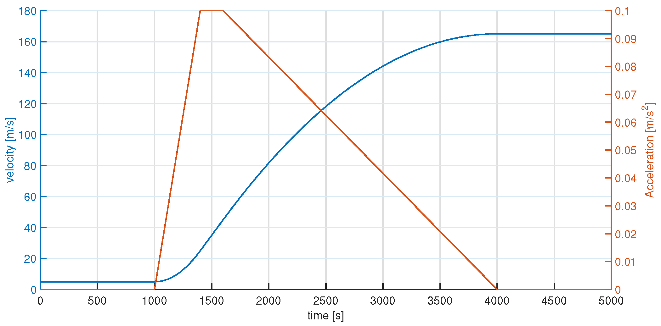
The considered case study is quite simple. A vehicle is moving at a velocity $v_{\mathrm{ref}}\left(t\right)$ with an acceleration $a_{\mathrm{ref}}\left(t\right)$, as shown in Figure 1.

The state equations of the vehicle can be written as:

$$\begin{array}{cc}\hfill & v_k=v_{k-1}+\tau ·a_{k-1}+w_k^v\hfill \\ \hfill & a_k=a_{k-1}+w_k^a\hfill \end{array}$$

(1)

• $v_k$ and $a_k$ are velocity and acceleration of the vehicle at time k;
• $w_k^v$ and $w_k^a$ are the standard deviation of the noise in velocity and acceleration respectively at time k;
• $\tau$ is the time period within two successive measurements

It is assumed that the noises are random in nature and belong to Gaussian distributions that do not vary with time (Gaussian distributions are considered as in [23], for a direct comparison). So, $w_k^v=w^v$ and $w_k^a=w^a$ are the standard deviations of the constant normal distributions with zero mean.

$w^v$ is assumed to be $0.003\mathrm{m}/\mathrm{s}$. This value has been derived by considering the accuracy of a GPS which has been reported in the official GPS website [24], which is usually quite accurate compared to the speedometer of the vehicle. Whereas, $w^a$ is assumed to be $0.0005\mathrm{m}/{\mathrm{s}}^2$ and is supposed to be due to some noise in the circuit or to the driver applying force on the accelerator.

The measured values of the velocity and the acceleration are supposed to have been obtained from the on board sensors of the vehicle. The accuracies of the onboard sensors are in general one or two magnitudes less accurate than a GPS based measurement. So, the following is considered:

• For the velocity, the random contribution is assumed to be normally distributed with a standard deviation of ${\sigma }_m^v=0.16\mathrm{m}/\mathrm{s}$. It has also been assumed that there is a residual systematic error in the measurement with an estimated value of $0.3\mathrm{m}/\mathrm{s}$. However, this is unknown and only an interval of possible values is known: $e_{sys}=\left[-0.32\mathrm{m}/\mathrm{s},+0.32\mathrm{m}/\mathrm{s}\right]$ has been assumed.
• For the acceleration, it has been assumed that there is no systematic error in the measurements and the random error is supposed to be normally distributed with a standard deviation of ${\sigma }_m^a=0.005\mathrm{m}/{\mathrm{s}}^2$.

3. Construction of the RFVs and the Possibilistic Kalman Filter

Although this has been explained in detail in [23], it has been recalled in this paper as the construction of the RFVs is the same also for the alternative possibilisitc KF defined in this paper.

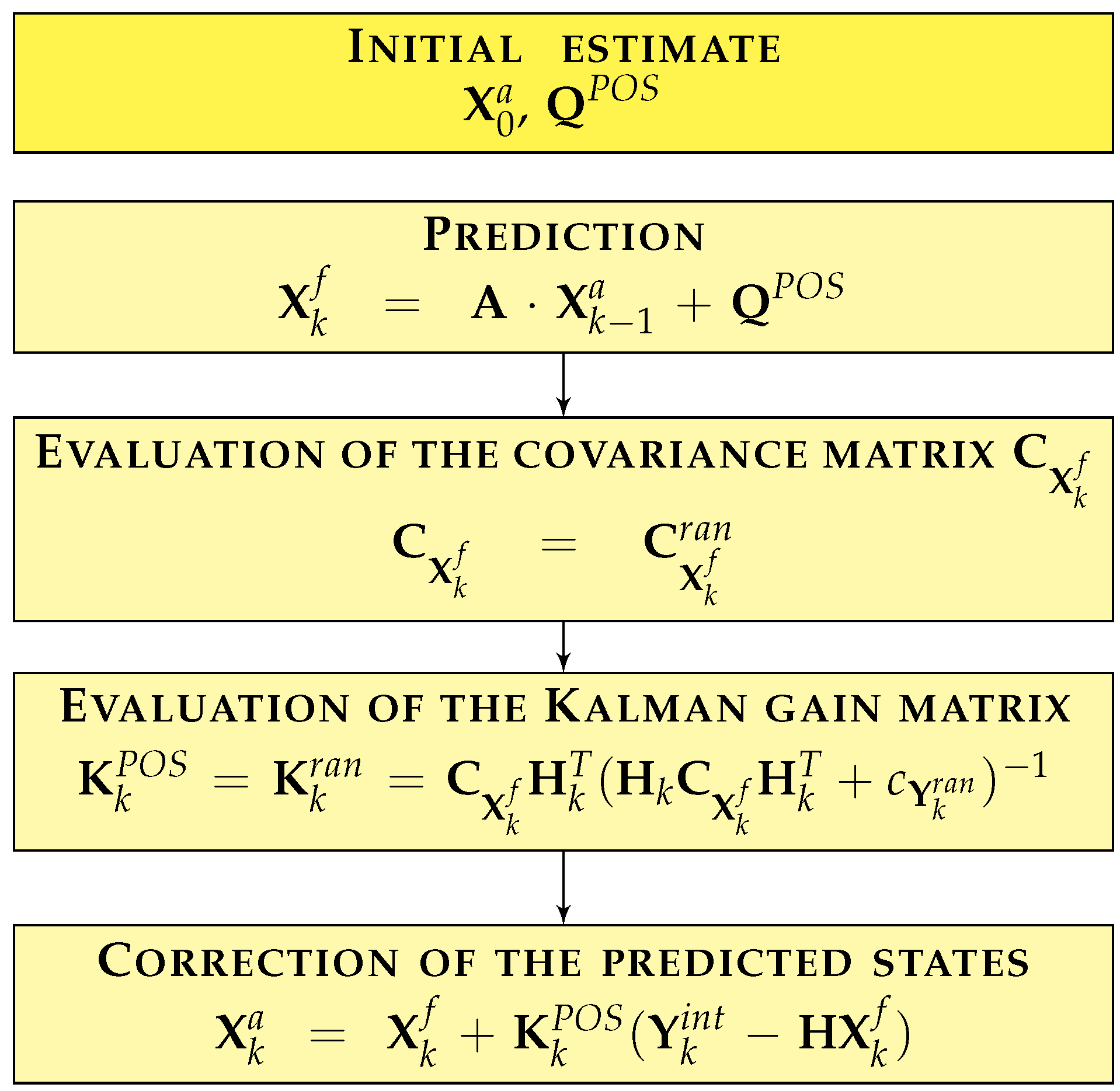
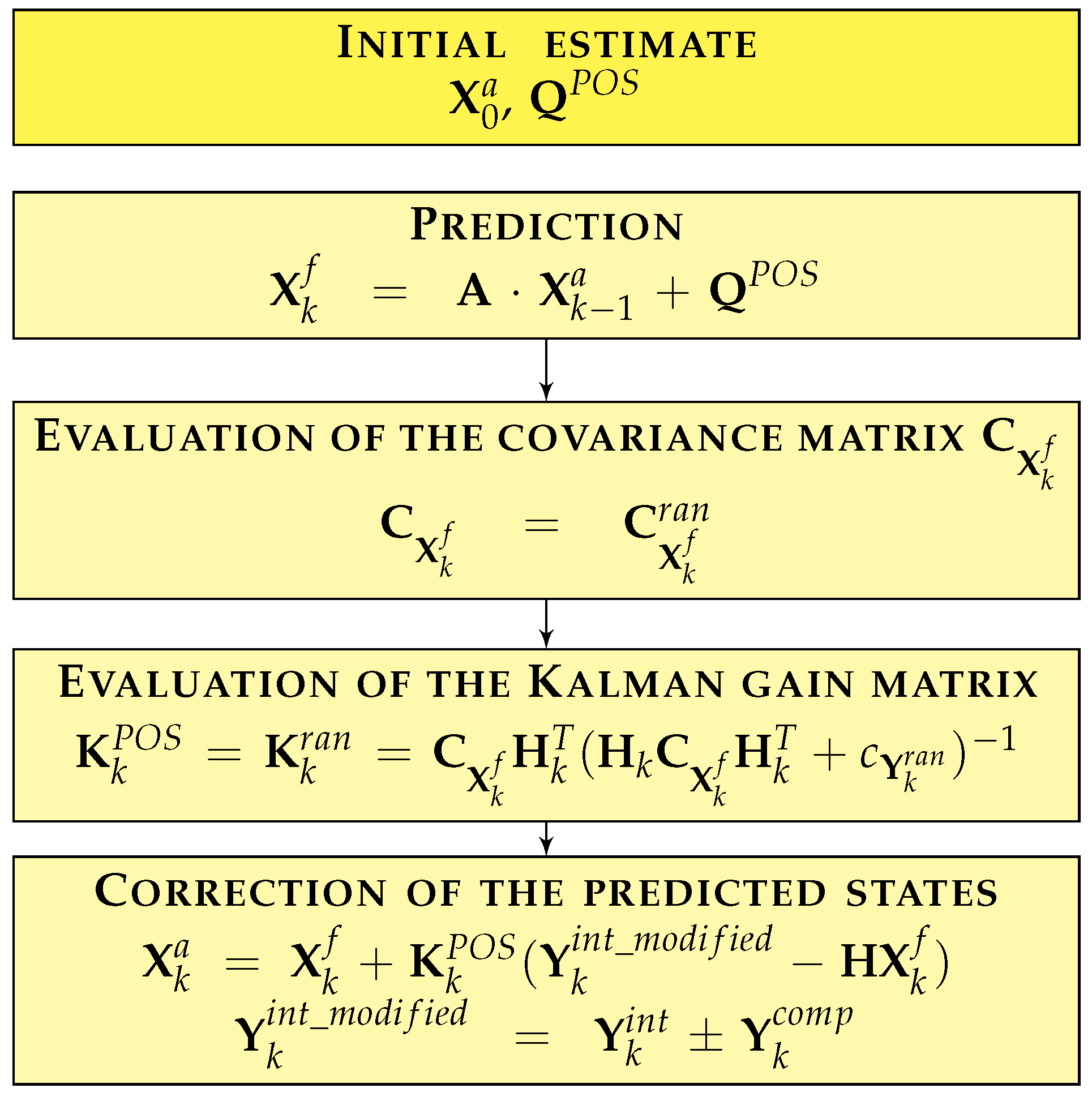
In the possibilistic KF defined in [23], all the states are RFVs and the algorithm is as shown in Figure 2 [23].

According to Equation (1): ${\mathbf{A}}_k=\mathbf{A}=\left[\begin{array}{cc}1& \tau \\ 0& 1\end{array}\right]$ and ${\mathbf{H}}_k=\mathbf{H}=\left[\begin{array}{cc}1& 0\\ 0& 1\end{array}\right]$.

Matrix ${\mathbf{Q}}^{POS}$ considers the model uncertainties and is a matrix of RFVs. According to the assumptions given in Section 2, we define ${\mathbf{Q}}^{POS}$ where:

• The element related to velocity is an RFV obtained by transforming the velocity noise variable into the possibility domain. Since there is no systematic error in the noise and the random part is assumed to be Gaussian, there is no internal possibility distribution (PD) in the RFV and the random PD is obtained by applying the probability-possibility transformation [16] on the zero mean normal probability density function (pdf) with standard deviation $w^v$ in the possibility domain;
• Similarly, the element related to acceleration is also an RFV in which there is no internal PD and the random PD is obtained by applying the probability-possibility transformation [16] on a zero mean normal pdf with standard deviation $w^a$ in the possibility domain;

As for the initial state vector ${\mathbf{X}}_0^a$, it is assumed that there are no systematic contributions to uncertainty. So, the RFV is obtained by just the random PD as follows:

• The initial velocity is an RFV consisting of just the random PD which is obtained by using the probability-possibility transformation [16] on a normal pdf with mean equal to the first measured value for velocity ($v_{m1}$) and standard deviation $w^v$;
• Similarly, the initial acceleration is an RFV consisting of just the random PD obtained by using the probability-possibility transformation [16] on a normal pdf with mean equal to the first measured value for acceleration ($a_{m1}$) and standard deviation $w^a$.

As for the measured values in each step k, matrix ${\mathbf{Y}}_k$ is the matrix of the RFVs of the velocity and acceleration measurements. The RFV associated with the simulated measured velocity is centered on the simulated measured velocity at step k ($v_{mk}$) and

• The internal PD is a rectangular PD with width $\pm e_{sys}$ around $v_{mk}$;
• the random PD is obtained by using the probability-possibility transformation [16] on a zero mean normal pdf, with standard deviation ${\sigma }_m^v$.

On the other hand, the acceleration has no systematic error. So, the RFV associated to the simulated measured acceleration is centered on the simulated measured acceleration at step k ($a_{mk}$) and

• the internal PD is zero;
• the random PD is obtained by using the probability-possibility transformation [16] on a normal pdf, with mean $a_k$ and standard deviation $u_{ran}^a$.

Matrix ${\mathbf{C}}_{{\mathbf{X}}_k^f}$ is the noise covariance matrix of the velocity and acceleration RFVs. However, as it is shown in the equations in Figure 2 and explained in [23], ${\mathbf{C}}_{{\mathbf{X}}_k^f}={\mathbf{C}}_{{\mathbf{X}}_k^f}^{ran}$. So, the possibilistic variances and covariances are evaluated from only the random contributions to uncertainty in both the velocity and acceleration RFVs.

Similarly, ${\mathbf{C}}_{{\mathbf{Y}}_k}={\mathbf{C}}_{{\mathbf{Y}}_k^{ran}}$ which means that the possibilistic variances and covariances of the noise covariance matrix associated with the measurements are evaluated from just the random uncertainty contributions in the velocity and acceleration measurements.

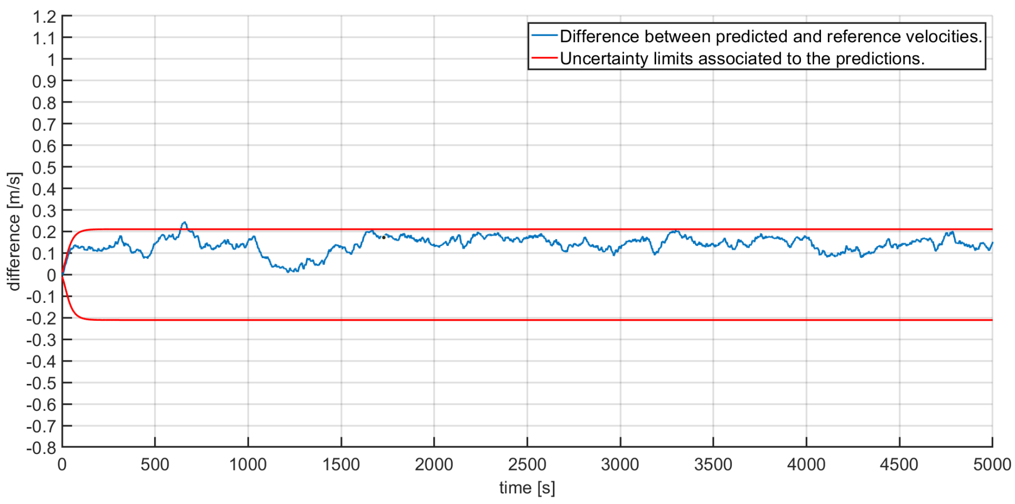
The described KF has been applied to the case study described in Section 2. The results obtained from the simulations are presented in Figure 3 and Figure 4.

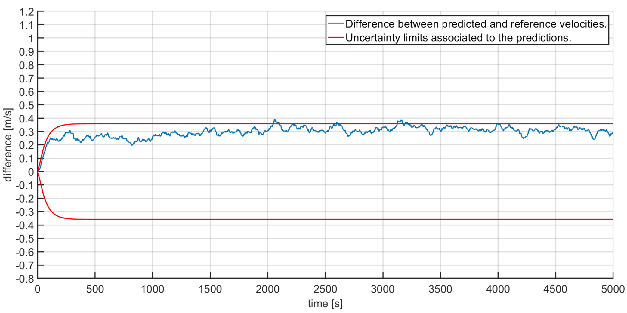
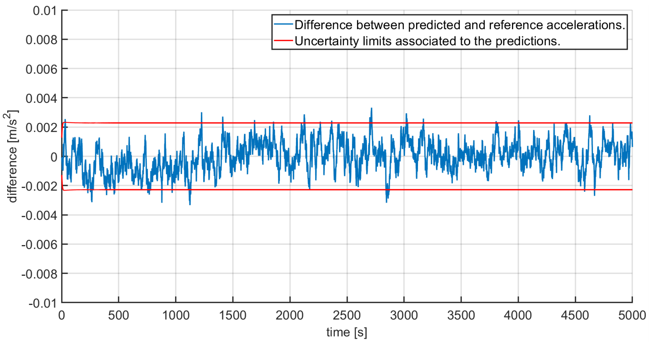
The predicted values of the velocity and acceleration from the KF are obtained by evaluating the mean values of the a posteriori RFVs in matrix ${\mathbf{X}}_k^a$. In both Figure 3 and Figure 4, the blue lines represent the differences in the predicted values given by the KF and the true values of the velocity and acceleration respectively.

The uncertainty limits associated to the state predictions (red lines) are the $\alpha -$cut at $\alpha =0.01$ of the velocity and acceleration RFVs predicted by the KF. The $\alpha -$cut can be considered as the confidence interval at the confidence level 1-$\alpha$[16]. For $\alpha =0.01$, these intervals correspond to the $99\%$ confidence interval in the corresponding pdf.

4. The Alternative Kalman filter Algorithm

In this paper, an alternative version of the KF algorithm described in Section 3 is presented, which allows for the reduction of the residual systematic error. As can be seen in the results in Figure 3 and Figure 4, the possibilistic KF algorithm described in Section 3 estimates the uncertainty intervals associated with the predictions very accurately in the presence of a systematic error. However, it does not compensate for the systematic error.

The alternative possibilistic KF which is proposed in this paper makes use of the above uncertainty interval to partially compensate for the systematic error. The new algorithm is synthetically shown in Figure 5. With respect to the algorithm in Figure 2, it can be seen that all steps are equal, except the last one, which corresponds to the “correction of the predicted states”.

In particular, a new RFV ${\mathbf{Y}}_k^{comp}$ is considered, which tries to compensate for the residual systematic error. At each step k, ${\mathbf{Y}}_k^{comp}$ consists of just the internal PD which is centered at the positive uncertainty limit evaluated by the KF at the previous iteration (step $k-1$) and with the same width and shape as the internal membership function of the RFVs of the state variables estimated by the KF in the previous iteration (${\mathbf{X}}_{k-1}^{int}$).

${\mathbf{Y}}_k^{int\_modified}$ is then obtained by adding or subtracting the RFV ${\mathbf{Y}}_k^{comp}$ from ${\mathbf{Y}}_k^{int}$, depending on if the systematic error is positive or negative:

$${\mathbf{Y}}_k^{int\_modified}=\left\{\begin{array}{cc}{\mathbf{Y}}_k^{int}+{\mathbf{Y}}_k^{comp}\hfill & \mathrm{if}\mathrm{systematic}\mathrm{error}<0\hfill \\ {\mathbf{Y}}_k^{int}-{\mathbf{Y}}_k^{comp}\hfill & \mathrm{if}\mathrm{systematic}\mathrm{error}>0\hfill \end{array}\right.$$

(2)

It is exactly like a negative feedback loop: the effects of the systematic contrbutions to uncertainty predicted by the KF is used as a feedback to compensate for a possible systematic error and the systematic error is partially compensated for. The intrinsic requirement for applying this method is that we know the direction of the systematic error i.e., it should be known if the error is positive or negative.

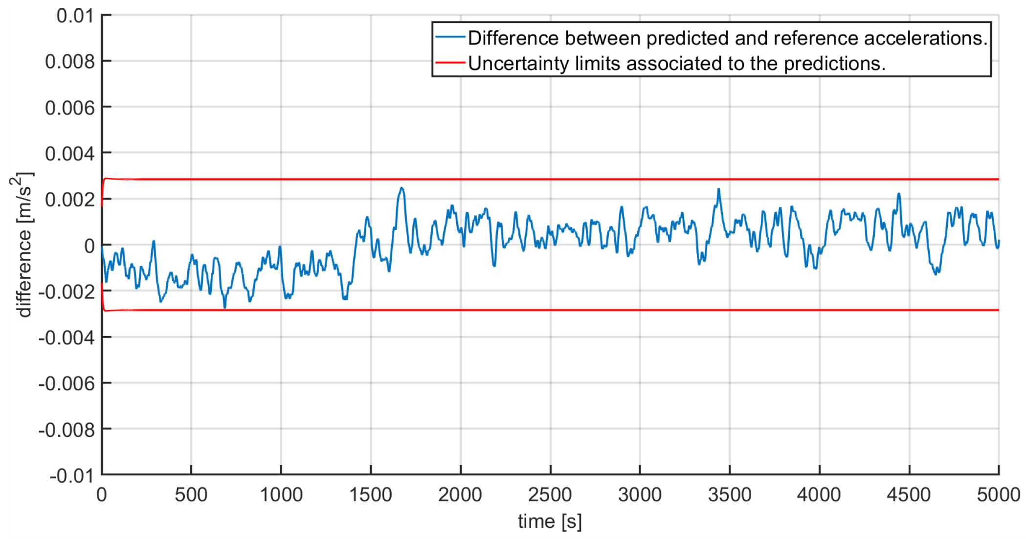
The obtained results are shown in Figure 6 and Figure 7. Again, the predicted values for the velocity and acceleration given by the KF are the mean values of the velocity and acceleration RFVs in matrix ${\mathbf{X}}_k^a$.

As in Figure 3 and Figure 4, also in Figure 6 and Figure 7 the blue lines represent the differences in the predicted values given by the KF and the true values of the velocity and acceleration respectively. The uncertainty limits associated the state predictions (red lines) are the $\alpha -cut$ at $\alpha =0.01$ of the velocity and acceleration RFVs predicted by the KF.

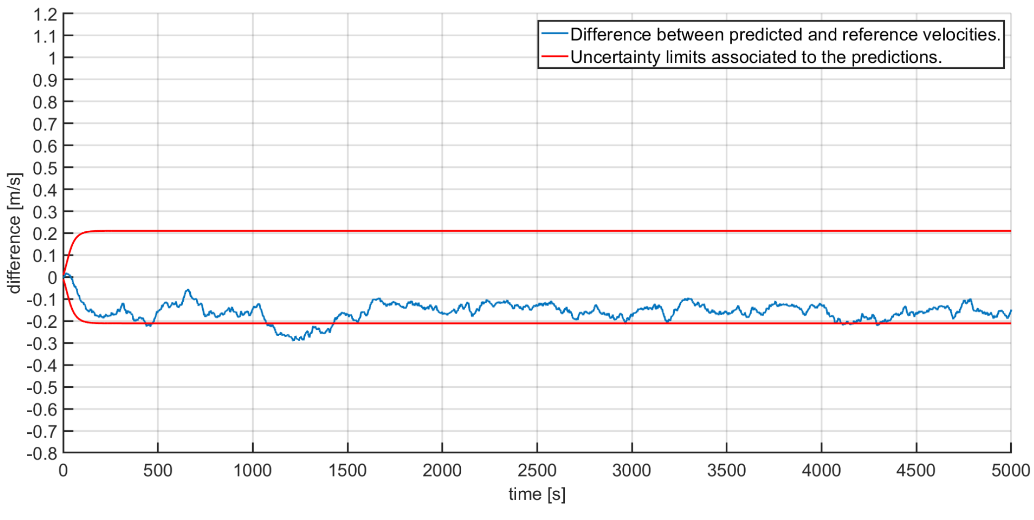
In Figure 6, with respect to Figure 3, it can be clearly seen that the uncertainty limits have been significantly reduced along with the residual systematic error in the velocity estimate.

Table 1. Comparison of synthetic indexes for the velocity.

KF	Possibilistic	Alternative Possibilistic
Convergence(s)	151	138
Steady-state error	0.3024	0.1696
Variation of error	0.0220	0.0257
Uncertainty limits	$\pm 0.3589$	$\pm 0.2106$
Variation of uncertainty limits	0	0
Percentage inside the uncertainty limits	99.00	95.88

gives a comparison with synthetic indexes for the velocity of the possibilistic KF and the alternative possibilistic KF.

5. Further Simulations

Further simulations have been performed in order to verify the effectiveness of the alternative possibilistic KF in all situations. In particular, we want to verify whether the algorithm still works in a good way when it is applied, but no residual systematic error is present.

In fact, the result of the introduction of the “feedback” loop is that the residual systematic error is compensated by the maximum possible value since the uncertainty limit of the RFVs evaluated in each step (which is the value of the $\alpha$-cut at $\alpha =0.01$ of the RFV) is considered. This means that it is possible that the residual systematic error could be overcompensated as the magnitude of this is unknown.

So, it is important that even if the residual systematic error happens to be zero (which is the limiting case), the overcompensation should not be so high that the predictions of the state variables obtained from the KF fall out of the evaluated uncertainty limits. To verify this, the same example described in the Section 2 is considered except that the systematic error is considered to be zero (instead of 0.3 m/s).

In this case, the results in Figure 8 and Figure 9 are obtained.

As expected, as can be seen in Figure 8, the systematic error in the velocity has been overcompensated, but it is still mostly inside the evaluated uncertainty limits. This demonstrates that the alternative possibilistic KF algorithm successfully decreases the uncertainty associated to the state predictions provided by the KF in all situations. In fact, the average uncertainty in Figure 8 is in any case smaller than the one in Figure 3.

6. Experimental Case Study

To validate the simulation results, a parrot AR drone has been used for the experimental case study. The drone has the following technical specifications as given by the manufacturer:

• 1 GHz 32 bit ARM Cortex processor with 800 MHz video DSP.
• 1 Gbit DDR2 RAM at 200 MHz.
• Wi-Fi b/g/n.
• 3 axis accelerometer +/−50 mg precision.
• 3 axis gyroscope 2000${}^{\circ }$ second precision.
• Pressure sensor +/−10 Pa precision.
• 60fps vertical QVGA camera.
• 3 axis magnetometer 6${}^{\circ }$ precision
• Ultrasound sensors.

The parrot AR drone has been developed as a low cost drone by parrot company and is quite customizable. The code is open source and can be modified according to the necessity. It has a variety of sensors and the data can be obtained from them and processed as needed. For the present case study, the velocity and acceleration measurements have been considered. For information about the algorithm used by the drone to calculate its speed, the readers are suggested to refer to [25].

The employed drone has been observed to have a negative systematic error in the velocity measurements obtained from the sensors present in the drone itself. So, the velocity is being underestimated by the sensors of the drone. It has also been observed that the systematic error is not constant for all runs. Each individual run had a systematic error that may be different from the other runs. So, only an interval of values can be estimated and the error can not just be compensated.

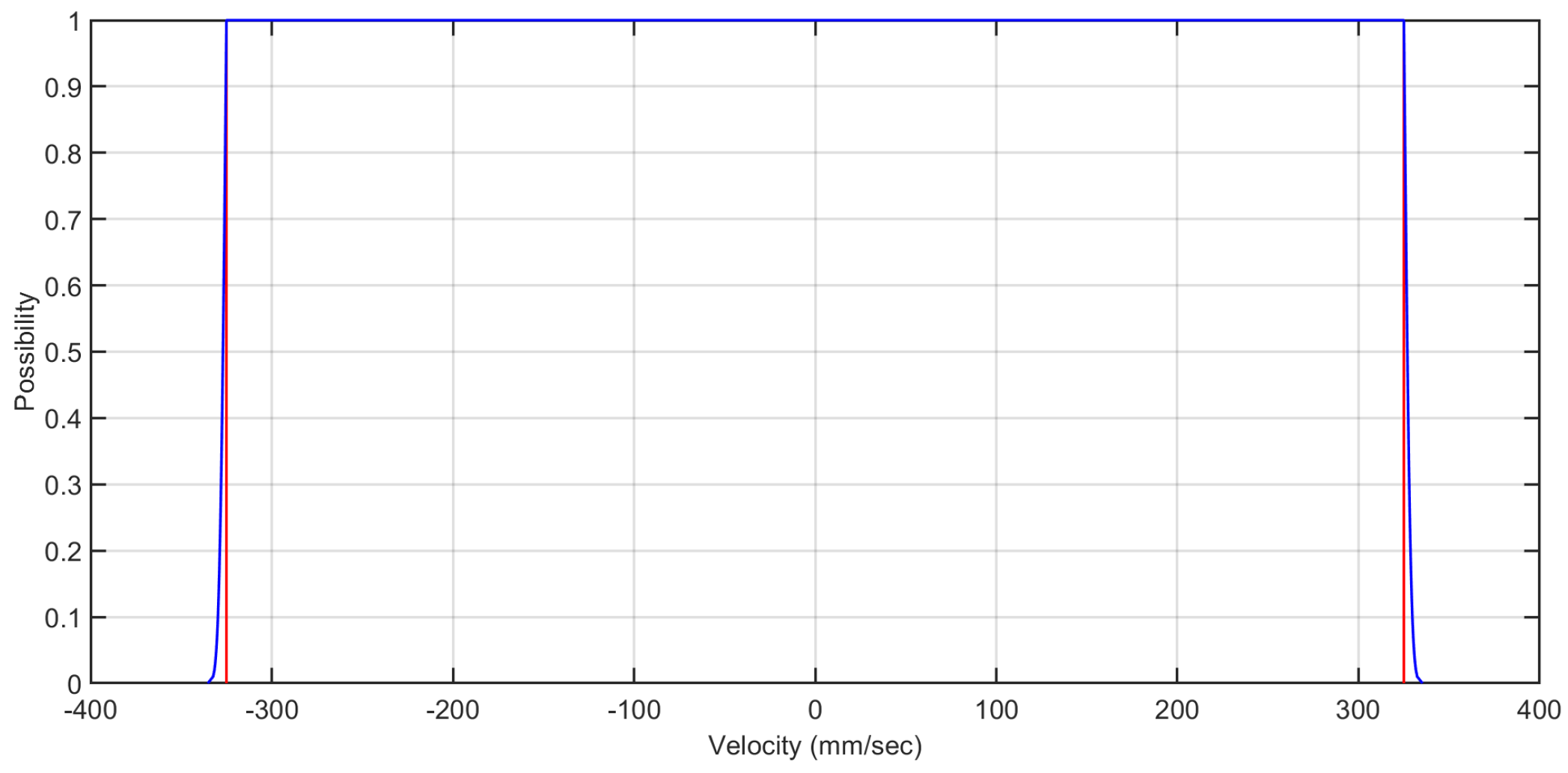
By performing a large number of runs of the drone, the interval for the systematic error has been estimated and this was used to construct the internal membership function of the RFV for the measured velocity. The constructed RFV assumed to be centered at zero velocity can be seen in Figure 10.

The measured acceleration, on the other hand, does not have any systematic contributions to uncertainty. Hence, the RFV can be constructed by simply using a probability-possibility transformation on the probability distribution of the acceleration.

The drone was made to fly for a few seconds to cover a distance of approximately 4 m. The velocity and acceleration data from the sensors is obtained from the drone every 5 ms using a software program that links the computer with the drone using the Wi-Fi network. The alternative possibilistic KF described in Section 4 was used to provide the filtered velocity and acceleration predictions with their respective uncertainties as well as compensate partially for the systematic error in the velocity measurements provided by the drone.

The velocity estimates provided by the KF were integrated to get the estimated distance traveled by the drone. Similarly, the velocity measurements directly obtained by the drone were integrated as well, to get the distance that the drone traveled according to the sensors present in the drone.

At the end of every run, the actual distance from the starting point was been measured. Measuring tape was used to do this since the error in the distance calculated using the velocity data from the sensors is quite high and the precision of the measuring tape is enough to be deemed negligible. Several runs were made and the distances estimated by the KF and those estimated according to the sensor data were compared with the actual distance traveled by the drone. To facilitate a comparison between the alternative KF defined in this paper and the possibilistic KF defined in [23], the sensor data was processed using both the KFs seperately.

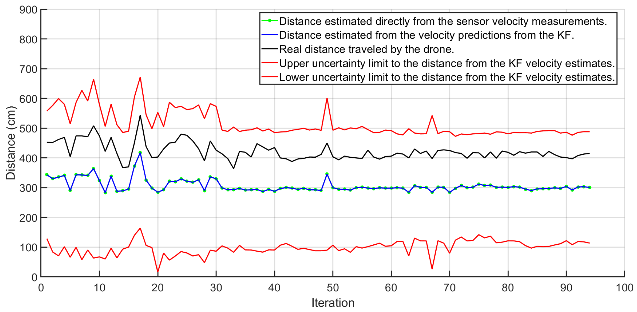
The results using the possibilistic KF defined in [23] can be seen in Figure 11. The green line represents the distances estimated according to the velocity measurements obtained directly from the sensors in the drone. The blue line represents the distance obtained from the velocity estimates of the defined possibilistic KF. The black line represents the actual distance traveled by the drone. Finally, the red lines represent the upper and lower bounds for the uncertainty.

It can be seen that the distances estimated by the possibilistic KF are quite close to the distances from the sensors. The blue line and the green line in Figure 11 are almost the same and that is why only the green dots and the blue line can be seen in the figure. However, the real measurements lie inside the uncertainty limits of the distances provided by the KF.

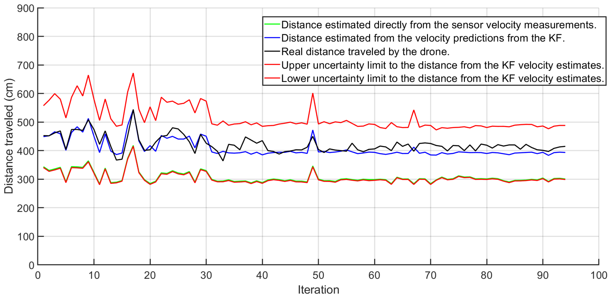
The results using the alternative KF defined in this paper can be seen in Figure 12. Again, the green line represents the distances estimated according to the velocity measurements obtained directly from the sensors in the drone. The blue line represents the distance obtained from the velocity estimates of the defined possibilistic KF. The black line represents the actual distance traveled by the drone. Finally, the red lines represents the upper and lower bounds for the uncertainty.

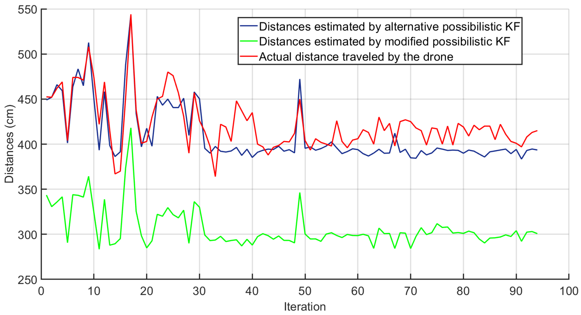
For an easier comparison, Figure 13 shows again the distances obtained using the modified possibilistic KF (green line) and those obtained using the alternative possibilistic KF (blue line) along with the actual distance traveled by the drone (red line).

A comparison of the results obtained from the two KFs has also been given in

Table 2. Comparison of the distance estimates of the drone obtained from the two KFs.

KF	Possibilistic	Alternative Possibilistic
Average error between the real distance and estimated distance	115.3273	12.4821
Mean width of the uncertainty band	$\pm 416.30$	$\pm 210.63$

. From Table 2, it can be clearly seen that the distance obtained using the alternative KF defined in this paper is much more accurate and closer to the real measurements than the distances obtained from the sensor measurements or those obtained from the possibilistic KF defined in [23].

Additionally, it can be easily seen that the width of the uncertainty limits associated with the distance (red lines) are also smaller in Figure 12 compared to that in Figure 11. The same can be verified from Table 2.

This confirms that the systematic error in the velocity is being compensated quite efficiently using the defined alternative possibilistic KF and the overall uncertainty associated to the predictions is being decreased as well.

7. Conclusions

The modified possibilistic KF defined in [23] is capable of propagating the systematic contributions to uncertainty effectively. This paper defines an alternative possibilistic KF which also decreases the effects of the systematic uncertainty contributions on the final measurement and therefore can be considered an improved version of the KF defined in [23].

The same simulated case study as in [23] has been considered to facilitate an easy comparison and the results obtained using the KF defined in this paper have been shown along with the results obtained by using the KF defined in [23]. The obtained results show that the proposed KF provides a compensation of the systematic uncertainty and decreases the overall uncertainty associated to the predictions.

The only requirement to use this method is that the direction of the residual systematic error should be known. This requirement is not so difficult to be satisfied in the era of big data. In any case, if not satisfied, the modified possibilistic KF defined in [23] is still valid and can be successfully applied. A possible area of application of the alternative possibilistic KF proposed in this paper could be in PTP networks where the network traffic is being monitored and thereby it can be evaluated if the transmission delay is higher from master to slave or from slave to master, thus identifying the direction of the systematic error in the calculation of the offset. Therefore, this method could be used to further decrease the uncertainty associated with the time predictions provided by the KF.

References

- Faragher, R. Understanding the basis of the kalman filter via a simple and intuitive derivation. IEEE Signal Process. Mag. 2012, 29, 128–132. [Google Scholar] [CrossRef]
- Wei, W.; Gao, S.; Zhong, Y.; Gu, C.; Subic, A. Random weighting estimation for systematic error of observation model in dynamic vehicle navigation. Int. J. Control Autom. Syst. 2016, 14, 514–523. [Google Scholar] [CrossRef]
- Yang, Y.; Rees, N.; Chuter, T. Reduction of encoder measurement errors in ukirt telescope control system using a kalman filter. IEEE Trans. Control Syst. Technol. 2002, 10, 149–157. [Google Scholar] [CrossRef]
- Noack, B.; Klumpp, V.; Hanebeck, U.D. State estimation with sets of densities considering stochastic and systematic errors. In Proceedings of the 12th International Conference on Information Fusion, Seattle, WA, USA, 6–9 July 2009. [Google Scholar]
- Novoselov, R.Y.; Herman, S.M.; Gadaleta, S.M.; Poore, A.B. Mitigating the effects of residual biases with schmidt-kalman filtering. In Proceedings of the 2005 7th International Conference on Information Fusion, Philadelphia, PA, USA, 25–28 July 2005; Volume 1, p. 8. [Google Scholar]
- Zhu, Q.; Jiang, Z.; Zhao, Z.; Wang, H. Uncertainty estimation in measurement of micromechanical properties using random-fuzzy variables. Rev. Sci. Instrum. 2006, 77, 035107. [Google Scholar] [CrossRef]
- Pertile, M.; Cecco, M.D.; Baglivo, L. Uncertainty evaluation in two-dimensional indirect measurement by evidence and probability theories. IEEE Trans. Instrum. Meas. 2010, 59, 2816–2824. [Google Scholar] [CrossRef]
- Pertile, M.; Cecco, M.D. Uncertainty evaluation for complex propagation models by means of the theory of evidence. Meas. Sci. Technol. 2008, 19, 1–10. [Google Scholar] [CrossRef]
- Lou, C.W.; Dong, M.C. A novel random fuzzy neural networks for tackling uncertainties of electric load forecasting. Electr. Power Energy Syst. 2015, 73, 34–44. [Google Scholar] [CrossRef]
- Tu, Y.; Zhou, X.; Gang, J.; Liechty, M.; Xu, J.; Lev, B. Administrative and market-based allocation mechanism for regional water resources planning. Resour. Conserv. Recycl. 2015, 95, 156–173. [Google Scholar] [CrossRef]
- Chen, D.; Chu, X.; Sun, X.; Li, Y. A new product service system concept evaluation approach based on information axiom in a fuzzy-stochastic environment. Int. J. Comput. Integr. Manuf. 2015, 28, 1–19. [Google Scholar] [CrossRef]
- Matìa, F.; Jiménez, A.; Al-Hadithi, B.M.; Rodrìguez-Losada, D.; Galán, R. The fuzzy kalman filter: State estimation using possibilistic techniques. Fuzzy Sets Syst. 2006, 157, 2145–2170. [Google Scholar] [CrossRef]
- Oussalah, M.; Schutter, J.D. Possibilistic kalman filtering for radar 2d tracking. Inf. Sci. 2000, 130, 85–107. [Google Scholar] [CrossRef]
- JCGM 100:2008. Evaluation of Measurement Data—Guide to the Expression of Uncertainty in Measurement, (GUM 1995 with Minor Corrections); Joint Committee for Guides in Metrology. 2008. Available online: http://www.bipm.org/en/publications/guides/gum.html (accessed on 12 June 2021).
- JCGM 200:2012. International Vocabulary of Metrology—Basic and General Concepts and Associated Terms (VIM 2008 with Minor Corrections); Joint Committee for Guides in Metrology. 2012. Available online: http://www.bipm.org/en/publications/guides/vim.html (accessed on 12 June 2021).
- Salicone, S.; Prioli, M. Measurement Uncertainty within the Theory of Evidence; Springer Series in Measurement Science and Technology; Springer: New York, NY, USA, 2018. [Google Scholar]
- Ferrero, A.; Salicone, S. A comparison between the probabilistic and possibilistic approaches: The importance of a correct metrological information. IEEE Trans. Instrum. Meas. 2018, 67, 607–620. [Google Scholar] [CrossRef]
- Ferrero, A.; Salicone, S. Uncertainty: Only one mathematical approach to its evaluation and expression? IEEE Trans. Instrum. Meas. 2012, 61, 2167–2178. [Google Scholar] [CrossRef]
- Mauris, G.; Lasserre, V.; Foulloy, L. A fuzzy approach for the expression of uncertainty in measurement. Measurement 2001, 29, 165–177. [Google Scholar] [CrossRef]
- Mauris, G.; Berrah, L.; Foulloy, L.; Haurat, A. Fuzzy handling of measurement errors in instrumentation. IEEE Trans. Instrum. Meas. 2000, 49, 89–93. [Google Scholar] [CrossRef]
- Urbanski, M.; Wasowsky, J. Fuzzy approach to the theory of measurement inexactness. Measurement 2003, 34, 67–74. [Google Scholar] [CrossRef]
- Ferrero, A.; Ferrero, R.; Salicone, S.; Jiang, W. The kalman filter uncertainty concept in the possibility domain. IEEE Trans. Instrum. Meas. 2019, 68, 4335–4347. [Google Scholar] [CrossRef]
- Ferrero, A.; Jetti, H.V.; Salicone, S. The possibilistic kalman filter: Definition and comparison with the available methods. IEEE Trans. Instrum. Meas. 2020, 77, 035107. [Google Scholar]
- GPS Accuracy. Available online: https://www.gps.gov/systems/gps/performance/accuracy/ (accessed on 28 May 2021).
- Bristeau, P.J.; Callou, F.; Vissière, D.; Petit, N. The navigation and control technology inside the ar. drone micro uav. IFAC Proc. Vol. 2011, 44, 1477–1484. [Google Scholar] [CrossRef] [Green Version]
Figure 1.
Reference values of velocity (blue line) and acceleration (red line) over time.
Figure 2.
The possibilistic Kalman filter algorithm [
23].
Figure 3.
Difference in the reference and predicted velocity values (blue line) provided by the possibilistic Kalman filter together with the predicted uncertainty interval (red lines).
Figure 4.
Difference in the reference and predicted acceleration values (blue line) provided by the possibilistic Kalman filter together with the predicted uncertainty interval (red lines).
Figure 5.
The alternative possibilistic Kalman filter algorithm.
Figure 6.
Difference in the reference and predicted velocity values (blue line) provided by the possibilistic Kalman filter defined in this paper, together with the predicted uncertainty interval (red lines).
Figure 7.
Difference in the reference and predicted acceleration values (blue line) provided by the possibilistic Kalman filter defined in this paper, together with the predicted uncertainty interval (red lines).
Figure 8.
Difference in the reference and predicted velocity values (blue line) provided by the alternative possibilistic KF, together with the predicted uncertainty interval (red lines) when residual systematic error is zero.
Figure 9.
Difference in the reference and predicted acceleration values (blue line) provided by the alternative possibilistic KF, together with the predicted uncertainty interval (red lines) when residual systematic error is zero.
Figure 10.
RFV of the velocity constructed from the data. The blue line represents the external membership function and the red line represents the internal membership function.
Figure 11.
Distances obtained from the velocity estimates of the possibilistic KF (blue line). The predicted uncertainty intervals (red lines). Actual distance traveled by the drone (black line) and distances estimated according to the velocity measurements obtained directly from the sensors in the drone (green line). Green line and blue line are almost the same.
Figure 12.
Distances obtained from the velocity estimates of the defined alternative possibilistic KF (blue line). The predicted uncertainty intervals (red lines). Actual distance traveled by the drone (black line) and distances estimated according to the velocity measurements obtained directly from the sensors in the drone (green line).
Figure 13.
Distances obtained from the velocity estimates of the defined alternative possibilistic KF (blue line). The distances obtained from the velocity estimates of the modified alternative possibilistic KF (green lines). Actual distance traveled by the drone (red line).