
The Statistical Power and Confidence of Some Key Comparison Analysis Methods to Correctly Identify Participant Bias


Abstract
:1. Introduction
2. Analysis of Measurement Comparisons
2.1. Models of Error in Measurement Comparisons
2.1.1. Common Mean Model (CM)
2.1.2. Fixed-Effects Model (FE)
2.1.3. Random-Effects Model (RE)
2.2. Comparison Analysis Methods
2.2.1. Common Mean with Largest Consistent Subset (CM-LCS)
2.2.2. Common Mean with Cut-Off (CM-CO)
2.2.3. Common Mean with Exclusion of Obvious Outliers (CM-OO)
2.2.4. Fixed Effects with Weighted Mean (FE-WM)
2.2.5. Fixed Effects with Bayesian Model Averaging (FE-BMA)
2.2.6. Random Effects with Mandel–Paule (RE-MP)
2.2.7. Random Effects with DerSimonian and Laird (RE-DL)
2.2.8. Random Effects with Hierarchical Bayes (RE-HB)
- :
- Gaussian with zero mean and standard deviation of ,
- :
- half-Cauchy with median equal to the median of the absolute differences between measured values and their median,
- :
- half-Cauchy with median equal to median of .
2.2.9. Linear Pool (LP)
2.2.10. Leave One Out (LOO)
3. Comparing Various Methods
3.1. Testing
- The true value of the artefact is set to zero. There is no loss of generality with this condition.
- Each participant’s measurement result has infinite degrees of freedom. This is not always true in practice, but for a key comparison, laboratories tend to put in more effort than usual to improve the confidence in their uncertainty budget, and this usually results in high effective degrees of freedom.
- Each participant’s measurement is subject to an error drawn from a Gaussian distribution. The error variance was determined by random variates drawn from a normalised chi-squared distribution with four degrees of freedom. This distribution was chosen as a fair representation of the range of values typically observed in BIPM comparisons—most uncertainties are close to the mean (in this case unity), there are several ‘good’ laboratories with small uncertainties, and the occasional participant with very large uncertainties. Previous work showed that the simulations are not sensitive to the shape of this distribution [29].
- Only one or two laboratories’ measurements are biased (subject to an unacknowledged error). This reflects the situation for key comparisons of mature scales, where the quantity has been compared before—probably by many of the same participants—and most of the sources of error are well known. The results of such comparisons may support new measurement claims.
3.1.1. Input Data Sets
- For a participant i with no bias, these numbers were generated in two steps:
- A value of was obtained from a chi-squared random number generator with degrees of freedom, normalised to have a mean of unity;
- was set to , where was obtained from a Gaussian random number generator with a mean of zero and variance .
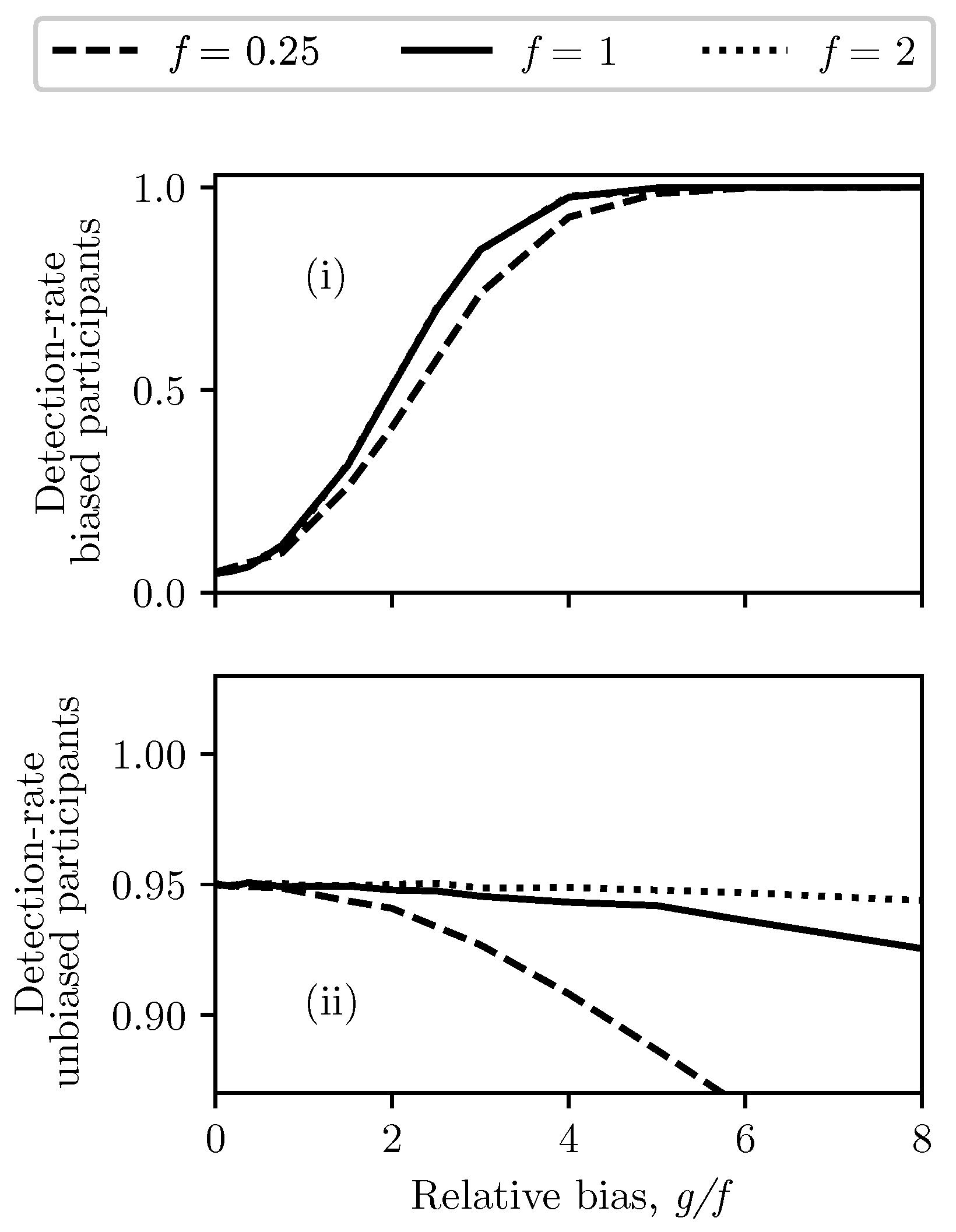
- For a biased participant, the generation of was controlled by two parameters f and g, which allowed us to configure various scenarios.
- was set to f;
- was set to , where was obtained from a Gaussian random number generator with a mean of zero and variance .
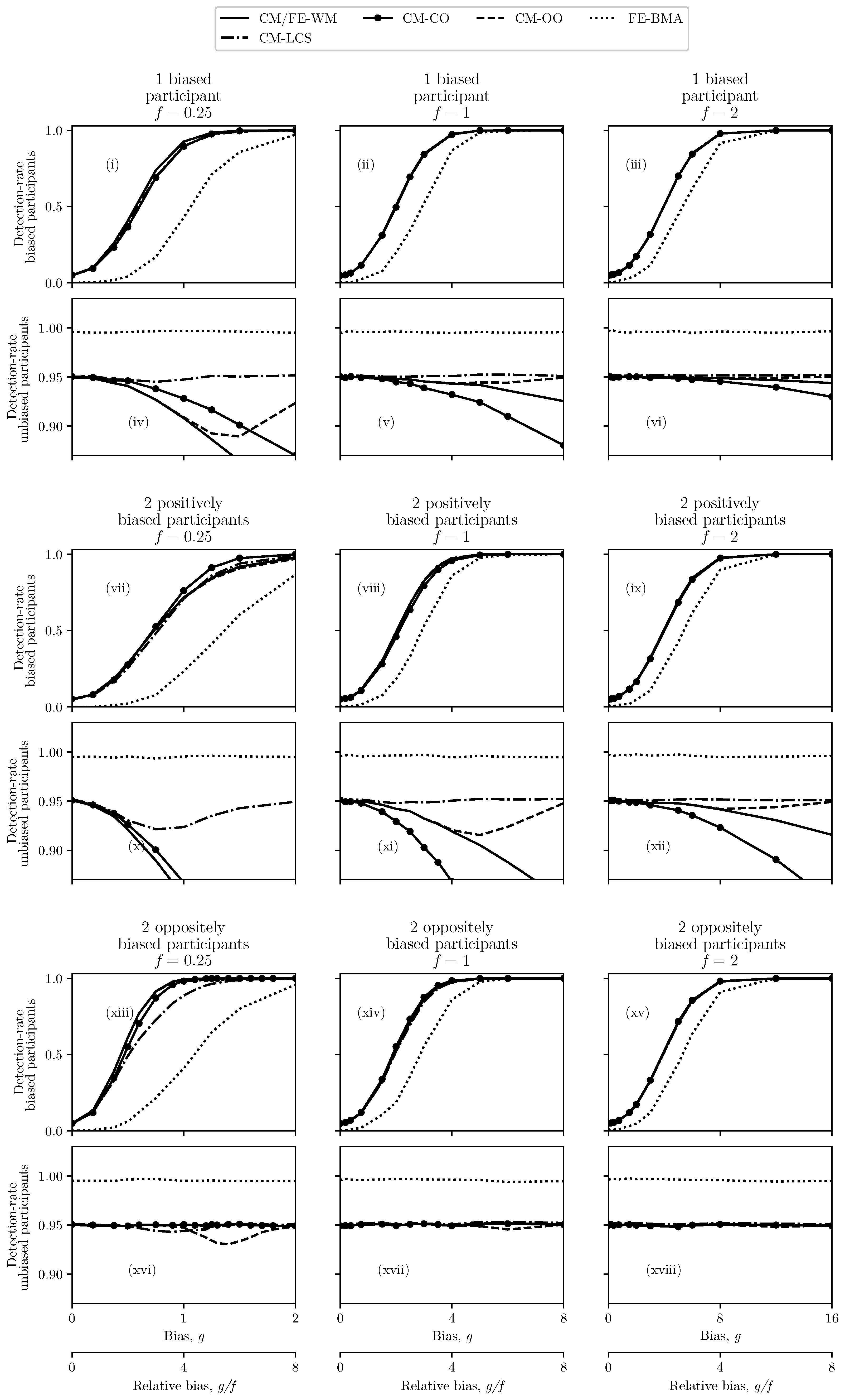
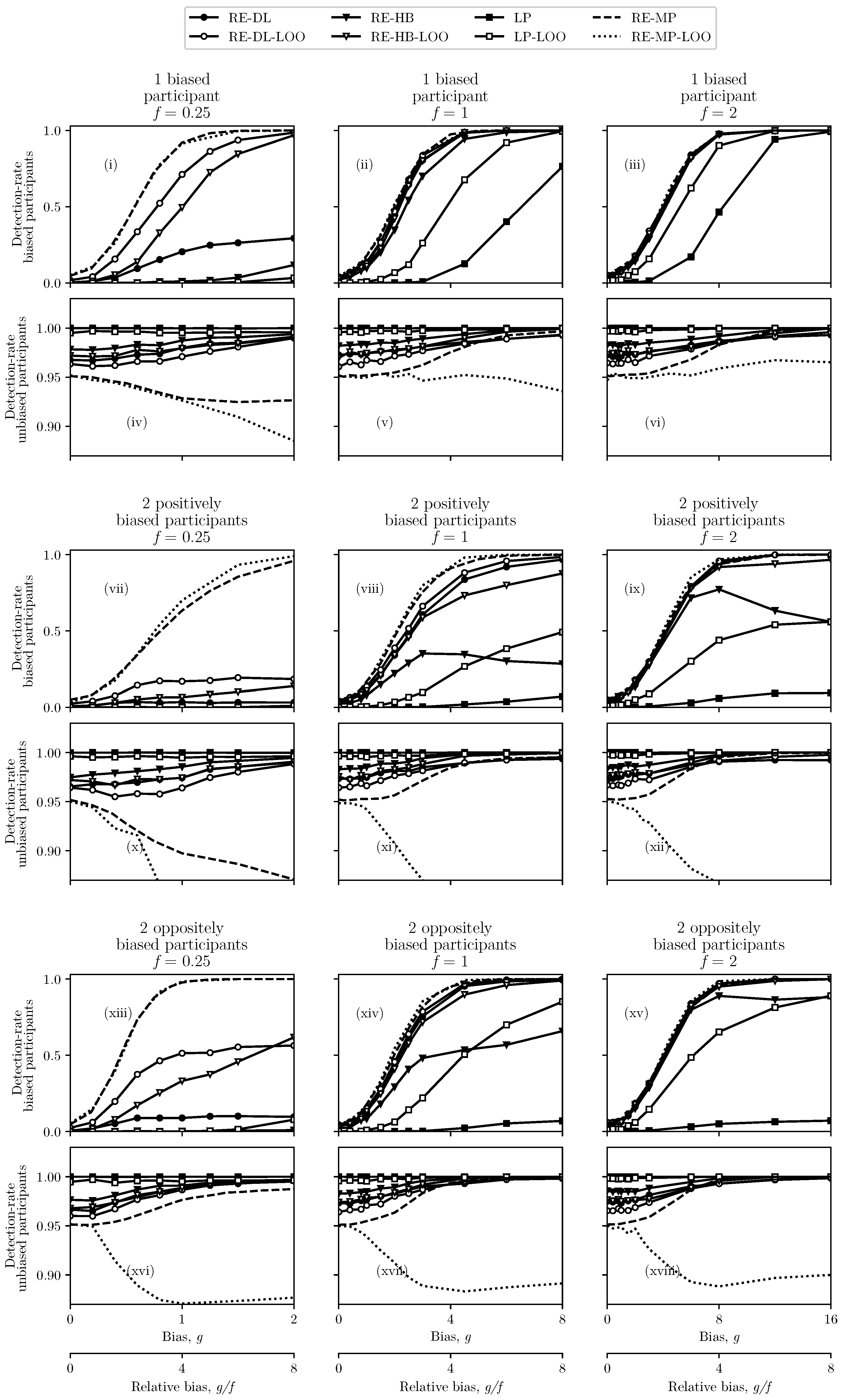
4. Results
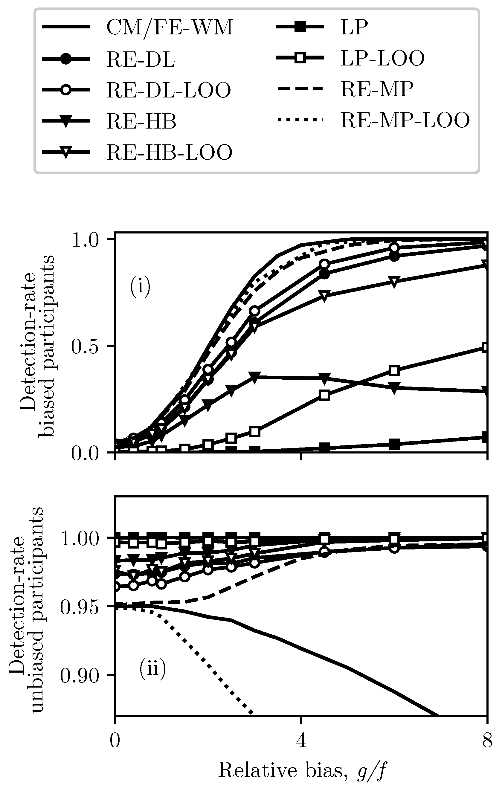
4.1. Unbiased Participants
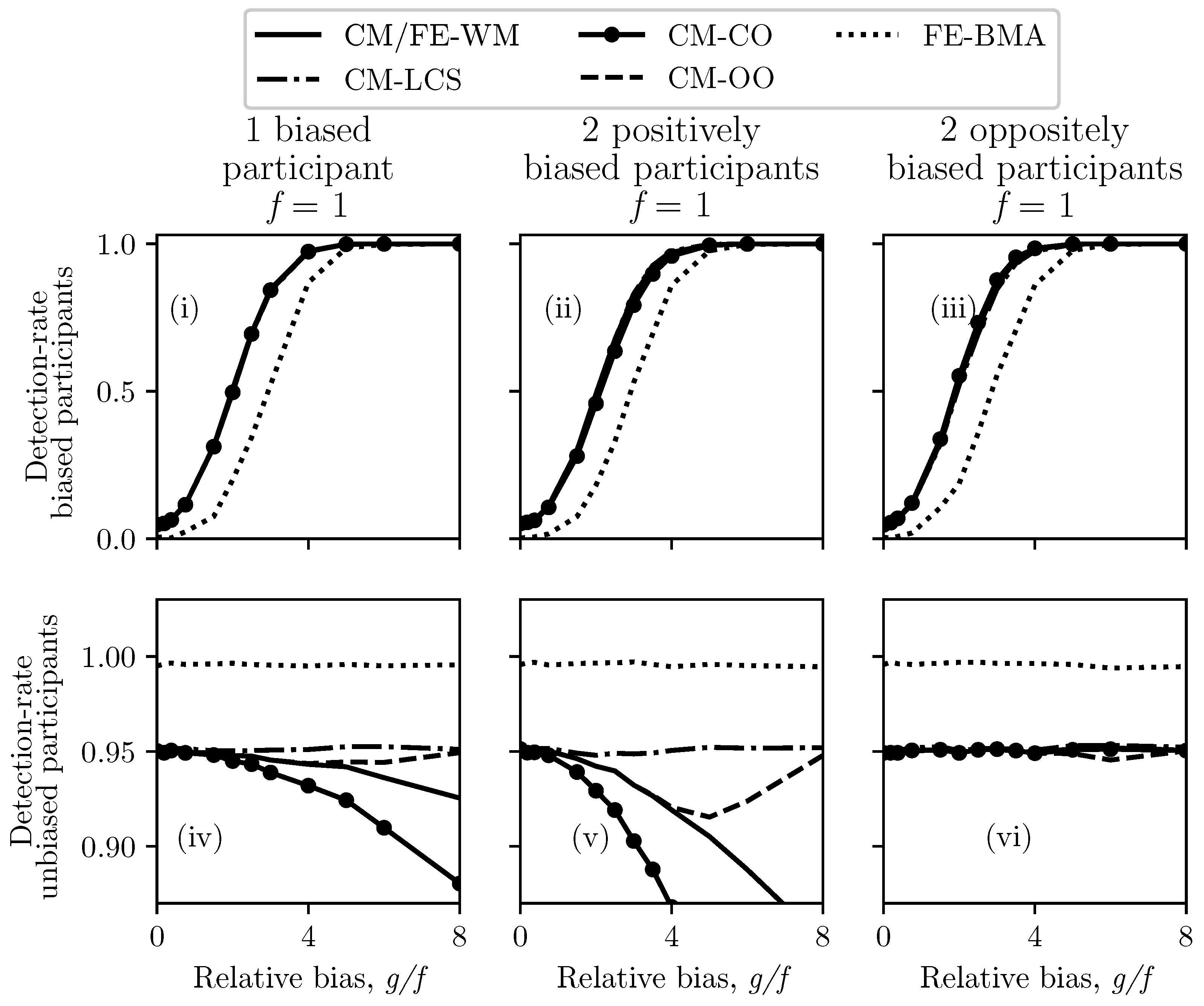
4.2. One or Two Biased Participants
- One positively biased participant,
- Two positively biased participants—with equal biases, and
- Two biased participants—with biases of equal magnitude and opposite sign.
5. Discussion
5.1. Method Assessment
5.2. Testing Applicability
5.3. Testing Conditions
6. Conclusions
Author Contributions
Funding
Data Availability Statement
Acknowledgments
Conflicts of Interest
Abbreviations
| BIPM | International Bureau of Weights and Measures |
| CM | Common Mean |
| CM-LCS | Common Mean with Largest Consistent Subset |
| CM-CO | Common Mean with Cut-Off |
| CM-OO | Common Mean with exclusion of Obvious Outliers |
| CCAUV | Consultative Committee for Acoustics, Ultrasound, and Vibration |
| CCEM | Consultative Committee for Electricity and Magnetism |
| CCQM | Consultative Committee for Amount of Substance |
| CCL | Consultative Committee for Length |
| CCM | Consultative Committee for Mass and Related Quantities |
| CCPR | Consultative Committee for Photometry and Radiometry |
| CIPM | International Committee for Weights and Measures |
| CMC | Calibration and Measurement Capability |
| DoE | Degree of Equivalence |
| FE | Fixed Effects |
| FE-BMA | Fixed Effects with Bayesian Model Averaging |
| FE-WM | Fixed Effects with Weighted Mean |
| LOO | Leave One Out |
| LP | Linear Pool |
| MRA | CIPM Mutual Recognition Arrangement |
| NMI | National Metrology Institute |
| RE-DL | Random Effects with DerSimonian and Laird |
| RE-HB | Random Effects with Hierarchical Bayes |
| RE-MP | Random Effects with Mandel–Paule |
Appendix A. Order Parameter Selection and Credible Interval Calculations for FE-BMA
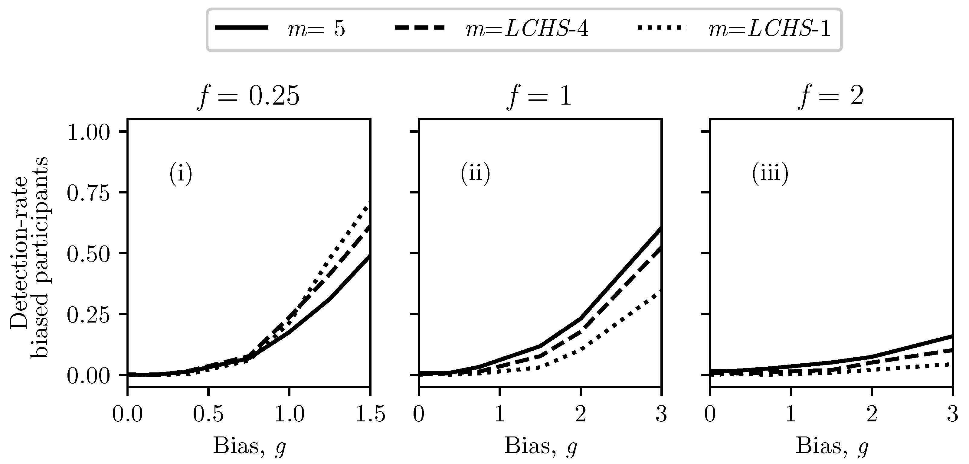
Appendix A.1. Order Parameter Selection

| m | Biased | Unbiased | Biased | Unbiased |
|---|---|---|---|---|
| 1 | 0.000 | 1.000 | 0.000 | 1.000 |
| 2 | 0.001 | 0.993 | 0.439 | 0.995 |
| 3 | 0.121 | 0.990 | 0.611 | 0.992 |
| 4 | 0.251 | 0.990 | 0.623 | 0.992 |
| 5 | 0.348 | 0.991 | 0.604 | 0.993 |
| 6 | 0.408 | 0.994 | 0.579 | 0.995 |
| 7 | 0.438 | 0.996 | 0.540 | 0.996 |
| 8 | 0.442 | 0.997 | 0.498 | 0.997 |
| 9 | 0.430 | 0.998 | 0.439 | 0.999 |
| 10 | 0.389 | 0.999 | 0.371 | 0.999 |
| 11 | 0.320 | 1.000 | 0.271 | 1.000 |

Appendix A.2. Credible Interval Calculations
Appendix B. Full Simulation Results


References
- CIPM. Technical supplement revised in October 2003. In Mutual Recognition of National Measurement Standards and of Calibration and Measurement Certificates Issued by National Metrology Institutes; BIPM: Sèvres, France, 2003; pp. 38–41. [Google Scholar]
- Willink, R. On the interpretation and analysis of a degree-of-equivalence. Metrologia 2003, 40, 9–17. [Google Scholar] [CrossRef]
- Wübbeler, G.; Bodnar, O.; Elster, C. Bayesian hypothesis testing for key comparisons. Metrologia 2016, 53, 1131–1138. [Google Scholar] [CrossRef]
- Cox, M.G. The evaluation of key comparison data. Metrologia 2002, 39, 589–595. [Google Scholar] [CrossRef]
- Cox, M.G. The evaluation of key comparison data: Determining the largest consistent subset. Metrologia 2007, 44, 187–200. [Google Scholar] [CrossRef]
- Toman, B.; Possolo, A. Laboratory effects models for interlaboratory comparisons. Accredit. Qual. Assur. 2009, 14, 553–563. [Google Scholar] [CrossRef]
- Elster, C.; Toman, B. Analysis of key comparisons: Estimating laboratories’ biases by a fixed effects model using Bayesian model averaging. Metrologia 2010, 47, 113–119. [Google Scholar] [CrossRef]
- Elster, C.; Toman, B. Analysis of key comparison data: Critical assessment of elements of current practice with suggested improvements. Metrologia 2013, 50, 549–555. [Google Scholar] [CrossRef]
- Lira, I. Bayesian evaluation of comparison data. Metrologia 2006, 43, 3–7. [Google Scholar] [CrossRef]
- Ballico, M. Calculation of key comparison reference values in the presence of non-zero-mean uncertainty distributions, using the maximum-likelihood technique. Metrologia 2001, 38, 155–159. [Google Scholar] [CrossRef] [Green Version]
- Willink, R. Meaning and models in key comparisons, with measures of operability and interoperability. Metrologia 2006, 43, S220. [Google Scholar] [CrossRef]
- Wübbeler, G.; Bodnar, O.; Mickan, B.; Elster, C. Explanatory power of degrees of equivalence in the presence of a random instability of the common measurand. Metrologia 2015, 52, 400–406. [Google Scholar] [CrossRef]
- Koo, A.; Clare, J. On the equivalence of generalized least-squares approaches to the evaluation of measurement comparisons. Metrologia 2012, 49, 340. [Google Scholar] [CrossRef]
- White, D.R. On the analysis of measurement comparisons. Metrologia 2004, 41, 122–131. [Google Scholar] [CrossRef]
- Koepke, A.; Lafarge, T.; Possolo, A.; Toman, B. NIST Consensus Builder—User’s Manual. 2017. Available online: https://consensus.nist.gov/app_{}direct/nicob/NISTConsensusBuilder-UserManual.pdf (accessed on 22 August 2021).
- Paule, R.C.; Mandel, J.; Bureau, N. Consensus Values and Weighting Factors. J. Res. Natl. Bur. Stand. 1982, 87, 377–385. [Google Scholar] [CrossRef]
- CIPM Consultative Committee for Photometry and Radiometry. CCPR-G2 Guidelines for CCPR Key Comparison Report Preparation. 2019. Available online: https://www.bipm.org (accessed on 22 August 2021).
- Koepke, A.; Lafarge, T.; Possolo, A.; Toman, B. Consensus building for interlaboratory studies, key comparisons, and meta-analysis. Metrologia 2017, 54, S34–S62. [Google Scholar] [CrossRef]
- Koo, A. Report on the consultative committee for photometry and radiometry key comparison of regular spectral transmittance 2010 (CCPR-K6.2010). Metrologia 2017, 54, 02001. [Google Scholar] [CrossRef]
- CIPM Consultative Committee for Mass and Related Quantities. Key Comparison Report Template v 1.3. 2019. Available online: https://www.bipm.org (accessed on 22 August 2021).
- CIPM Consultative Committee for Length. CCL-GD-3.2: Key Comparison Report Template. Available online: https://www.bipm.org (accessed on 22 August 2021).
- CIPM Consultative Committee for Amount of Substance. CCQM Guidance Note: Estimation of a Consensus KCRV and Associated Degrees of Equivalence. 2013. Available online: https://www.bipm.org (accessed on 22 August 2021).
- CIPM Consultative Committee for Electricity and Magnetism. CCEM Guidelines for Planning, Organizing, Conducting and Reporting Key, Supplementary and Pilot Comparisons. 2017. Available online: https://www.bipm.org (accessed on 22 August 2021).
- CIPM Consultative Committee for Acoustics Ultrasound and Vibration. Guidance for Carrying out Key Comparisons within the CCAUV. 2015. Available online: https://www.bipm.org (accessed on 22 August 2021).
- CIPM Consultative Committee for Ionizing Radiation. Key Decisions of the CCRI and CCRI Sections. 2019. Available online: https://www.bipm.org (accessed on 22 August 2021).
- Werner, L. Final report on the key comparison CCPR-K2.c-2003: Spectral responsivity in the range of 200 nm to 400 nm. Metrologia 2014, 51, 02002. [Google Scholar] [CrossRef]
- DerSimonian, R.; Laird, N. Meta-analysis in clinical trials revisited. Contemp. Clin. Trials 2015, 45, 139–145. [Google Scholar] [CrossRef] [PubMed] [Green Version]
- Whitehead, A.; Whitehead, J. A general parametric approach to the meta-analysis of randomized clinical trials. Stat. Med. 1991, 10, 1665–1677. [Google Scholar] [CrossRef] [PubMed]
- Molloy, E.; Koo, A. Methods and Software for Analysing Measurement Comparisons; Technical Report 0689; Callaghan Innovation: Lower Hutt, New Zealand, 2020. [Google Scholar] [CrossRef]
- Koo, A.; Harding, R.; Molloy, E. A Statistical Power Study of the NIST Consensus Builder Models to Identify Participant Bias in Comparisons; Technical Report 0805; Callaghan Innovation: Lower Hutt, New Zealand, 2020. [Google Scholar] [CrossRef]
- Possolo, A.; Koepke, A.; Newton, D.; Winchester, M.R. Decision tree for key comparisons. J. Res. Natl. Inst. Stand. Technol. 2021, 126, 126007. [Google Scholar] [CrossRef]


| Method | Equivalent |
|---|---|
| CM/FE-WM | 0.94949 (63) |
| CM-LCS | 0.95073 (62) |
| CM-CO | 0.94970 (63) |
| CM-OO | 0.94949 (63) |
| FE-BMA | 0.99558 (61) |
| RE-MP | 0.95111 (62) |
| RE-MP-LOO | 0.95142 (62) |
| RE-DL | 0.9709 (15) |
| RE-DL-LOO | 0.9644 (17) |
| RE-HB | 0.9818 (12) |
| RE-HB-LOO | 0.9732 (15) |
| LP | 0.99988 (10) |
| LP-LOO | 0.99619 (56) |
Publisher’s Note: MDPI stays neutral with regard to jurisdictional claims in published maps and institutional affiliations. |
© 2021 by the authors. Licensee MDPI, Basel, Switzerland. This article is an open access article distributed under the terms and conditions of the Creative Commons Attribution (CC BY) license (https://creativecommons.org/licenses/by/4.0/).
Share and Cite
Molloy, E.; Koo, A.; Hall, B.D.; Harding, R. The Statistical Power and Confidence of Some Key Comparison Analysis Methods to Correctly Identify Participant Bias. Metrology 2021, 1, 52-73. https://doi.org/10.3390/metrology1010004
Molloy E, Koo A, Hall BD, Harding R. The Statistical Power and Confidence of Some Key Comparison Analysis Methods to Correctly Identify Participant Bias. Metrology. 2021; 1(1):52-73. https://doi.org/10.3390/metrology1010004
Chicago/Turabian StyleMolloy, Ellie, Annette Koo, Blair D. Hall, and Rebecca Harding. 2021. "The Statistical Power and Confidence of Some Key Comparison Analysis Methods to Correctly Identify Participant Bias" Metrology 1, no. 1: 52-73. https://doi.org/10.3390/metrology1010004