Development and Practical Applications of Computational Intelligence Technology

Abstract

Computational intelligence (CI) uses applied computational methods for problem-solving inspired by the behavior of humans and animals. Biological systems are used to construct software to solve complex problems, and one type of such system is an artificial immune system (AIS), which imitates the immune system of a living body. AISs have been used to solve problems that require identification and learning, such as computer virus identification and removal, image identification, and function optimization problems. In the body’s immune system, a wide variety of cells work together to distinguish between the self and non-self and to eliminate the non-self. AISs enable learning and discrimination by imitating part or all of the mechanisms of a living body’s immune system. Certainly, some deep neural networks have exceptional performance that far surpasses that of humans in certain tasks, but to build such a network, a huge amount of data is first required. These networks are used in a wide range of applications, such as extracting knowledge from a large amount of data, learning from past actions, and creating the optimal solution (the optimization problem). A new technique for pre-training natural language processing (NLP) software ver.9.1by using transformers called Bidirectional Encoder Representations (BERT) builds on recent research in pre-training contextual representations, including Semi-Supervised Sequence Learning, Generative Pre-Training, ELMo (Embeddings from Language Models), which is a method for obtaining distributed representations that consider context, and ULMFit (Universal Language Model Fine-Tuning). BERT is a method that can address the issue of the need for large amounts of data, which is inherent in large-scale models, by using pre-learning with unlabeled data. An optimization problem involves “finding a solution that maximizes or minimizes an objective function under given constraints”. In recent years, machine learning approaches that consider pattern recognition as an optimization problem have become popular. This pattern recognition is an operation that associates patterns observed as spatial and temporal changes in signals with classes to which they belong. It involves identifying and retrieving predetermined features and rules from data; however, the features and rules here are not logical information, but are found in images, sounds, etc. Therefore, pattern recognition is generally conducted by supervised learning. Based on a new theory that deals with the process by which the immune system learns from past infection experiences, the clonal selection of immune cells can be viewed as a learning rule of reinforcement learning.

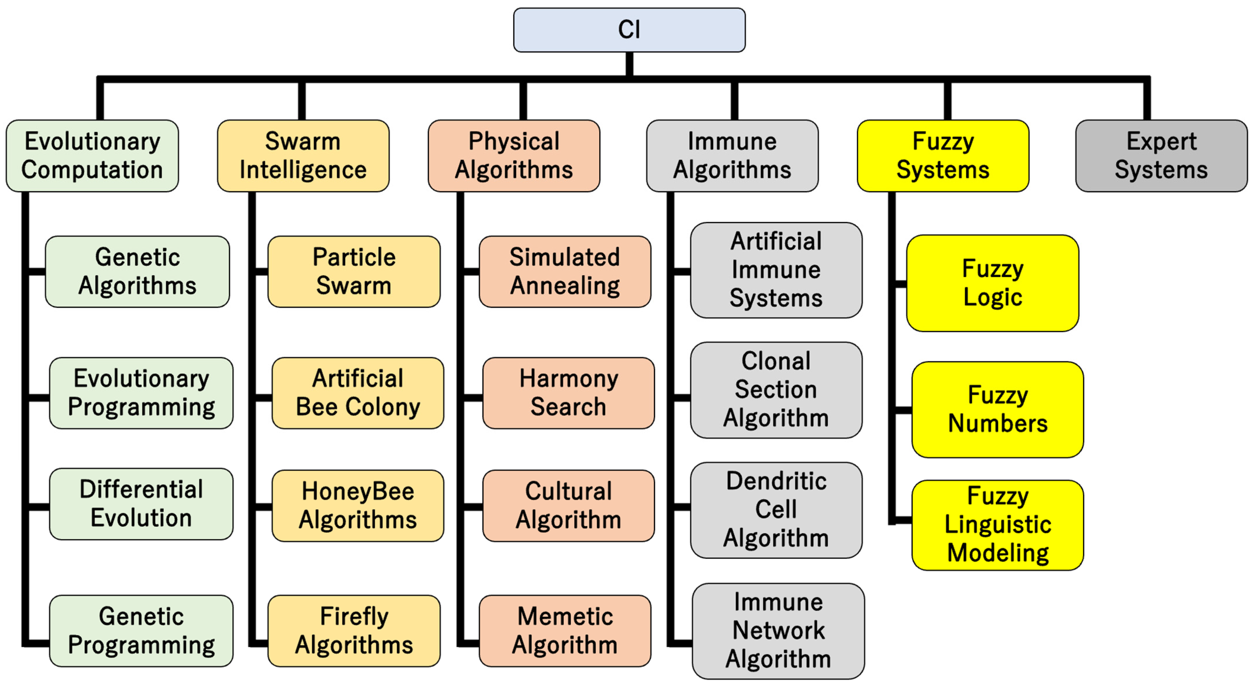
1. Introduction

CI research centers on heuristic algorithms such as fuzzy systems, neural networks, soft computing, chaos theory, genetic algorithms, swarm intelligence, fractals, artificial immune systems (AISs), wavelets, and evolutionary computation, and aims to create intelligent programs in a sense by making full use of elements such as learning, adaptation, evolution, and fuzzy logic (Figure 1) [1,2,3,4,5]. There are many algorithms inspired by phenomena in the natural world and they are characterized by being able to find a practical approximate solution in a short calculation time instead of an exact solution. CI is a branch of artificial intelligence (AI) research that is distinct from conventional AI based on mathematical logic, and involves the ability to recognize and understand objects by constructing models based on various phenomena and the data obtained from them using computational means [6]. Conventional AI, which is called logical AI or symbolic AI, learns a large amount of case data and performs logical processing. This can be called orthodox AI. However, a problem with orthodox AI is that even if the idea were extended, the calculations would only become more advanced and complicated, and it would not be possible to say that it would come close to “true intelligence”. CI, on the other hand, is an AI technology modeled on living organisms and natural phenomena, represented by neural networks, that has emerged in recent years. CI involves a wide range of concepts, including current AI, biological evolution models, the active introduction of human subjectivity (fuzzy logic), complex systems such as chaos and fractals, and multiagent distributed AI, which often refers to deep neural networks, especially convolutional neural networks, known as data-driven networks, which are trained using abundant and high-quality data. Fuzzy control is a type of control that uses fuzzy sets that allow intermediate states, unlike normal sets in which a point either belongs to a certain set or not, to construct a control model or control system. This allows intermediate values to be associated with ambiguous natural language expressions.

CI technology includes not only the construction of those models, but also technology to solve various problems by applying various computational methods. CI research does not reject statistical methods and often offers complementary ideas. For example, to determine the maximum and minimum values of a function, the function’s differential information is used. On the other hand, in the real world, there are many problems that are extremely difficult to differentiate or cannot be differentiated in the first place. Most CIs do not require differential information, so they are characterized by their applicability in various fields. Another advantage is that many algorithms are simple and easy to implement in simulations. CI is an applied computational method for problem solving inspired by the behavior of humans and animals. It is used in a wide range of applications, including extracting knowledge from a large amount of data, learning from past actions, and creating the optimal solution to the optimization problem.

Machine learning is a technique for building models, and optimization calculation is a technique for solving problems using models. The relationship between modeling and optimization is mutually complementary and inclusive. Neural network research is part of CI research and is closely related to machine learning. In recent years, CI has been applied not only to engineering and industrial problem solving, but also to various industrial fields, as well as in social problem solving such as in economics, medicine, and the environment, which is essential to expand its application area. In addition, a fuzzy system is a system of variables that are related using fuzzy logic. A fuzzy controller uses defined rules to control a fuzzy system based on the current values of input linguistic variables that are used to design and control fuzzy systems using Fuzzy System Designer and Fuzzy Logic VI.2.

2. Immune System and Computer System

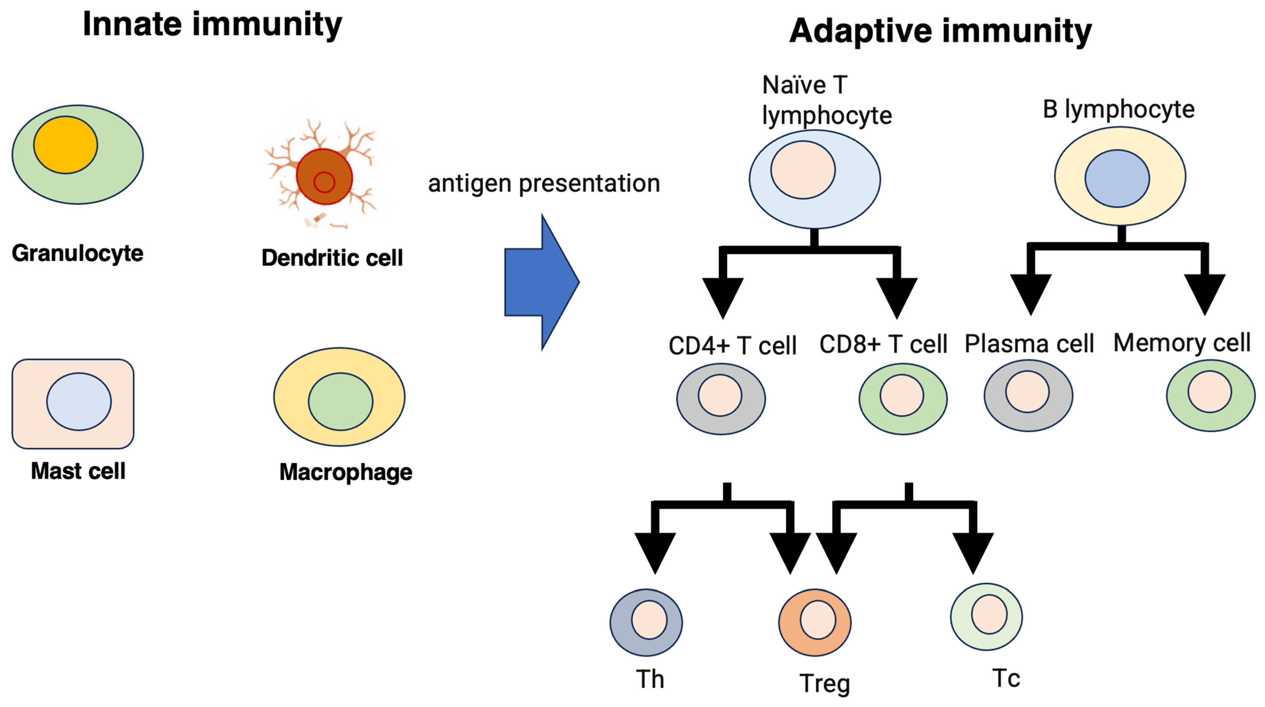
2.1. Immune System In Vivo

The body’s immune system distinguishes between the self and non-self, foreign substances, and the eliminated non-self. The immune system can be broadly divided into two mechanisms: the innate immune system and the adaptive immune system (Figure 2) [7,8,9]. The innate and acquired immune systems are mechanisms that respond nonspecifically or specifically to foreign substances, respectively. In the adaptive immune system, cells with various roles work together, with B cells, antigen-presenting cells, and T cells playing particularly important roles. Antigen-presenting cells capture antigens, which are foreign substances that have entered the body, and present antigen information to helper T cells. This immune system becomes activated when presented with antigen information and sends activation signals as information transmitters to each cell. When B cells receive activation signals from helper T cells, they produce antibodies, which neutralize antigens. If more antibodies are produced than are necessary, it will cause abnormalities in the body. Therefore, it is necessary to control the production of antibodies, and this control is performed by suppressor T cells.

In addition to the antigen elimination mechanism induced by B cells, the adaptive immune system includes antigen elimination by killer T cells. Killer T cells receive activation signals from helper T cells and are activated, thereby enhancing the elimination of encountered antigens. Suppressor T cells also control this elimination mechanism. Although most B cells and T cells die after eliminating antigens, some survive and circulate throughout the body as memory cells. These memory cells quickly mount an immune reaction to the subsequent invasion of similar antigens.

In addition, T cells, which play an important role in the adaptive immune system, can distinguish between the self and non-self against various antigens and eliminate the non-self. This is due to the diversity of the T cell receptor (TCR) of T cells, which is a receptor located on the T cell membrane and can identify various antigen patterns. This receptor functions when antigen information is presented by antigen-presenting cells. In addition to TCR, the T cell membrane contains CD4 and CD8 molecules. Helper or killer T cells have CD4 or CD8 molecules on their membrane surface, and without CD4 or CD8 molecules, they cannot function as helper or killer T cells. T cells distinguish between the self and non-self using TCR, CD4, and CD8 molecules when presenting antigens. Antigen-presenting cells add peptides, which are fragments of antigen information, to major histocompatibility complex (MHC) class I and class II proteins and present antigens to T cells. T cells can identify a variety of antigens because of the diversity of the TCR, which consists of two regions: a variable region accountable for antigen identification and a constant region. T cells perform identification by matching the pattern of the peptide presented by the antigen with the pattern of the variable region of the TCR.

The diversity of TCRs is achieved through a mechanism called gene rearrangement. In gene rearrangement, the required number of genes is randomly selected from many V, D, and J gene groups and connected to the C gene region, which allows TCR to achieve diversity. Gene rearrangements also occur in CD4 and CD8 molecules, antibodies, and MHC class I and class II proteins, which are the substances that affect helper and killer T cells. The TCR, CD4, CD8, and MHC class I and class II proteins produced by gene rearrangement are collectively called immunoglobulins.

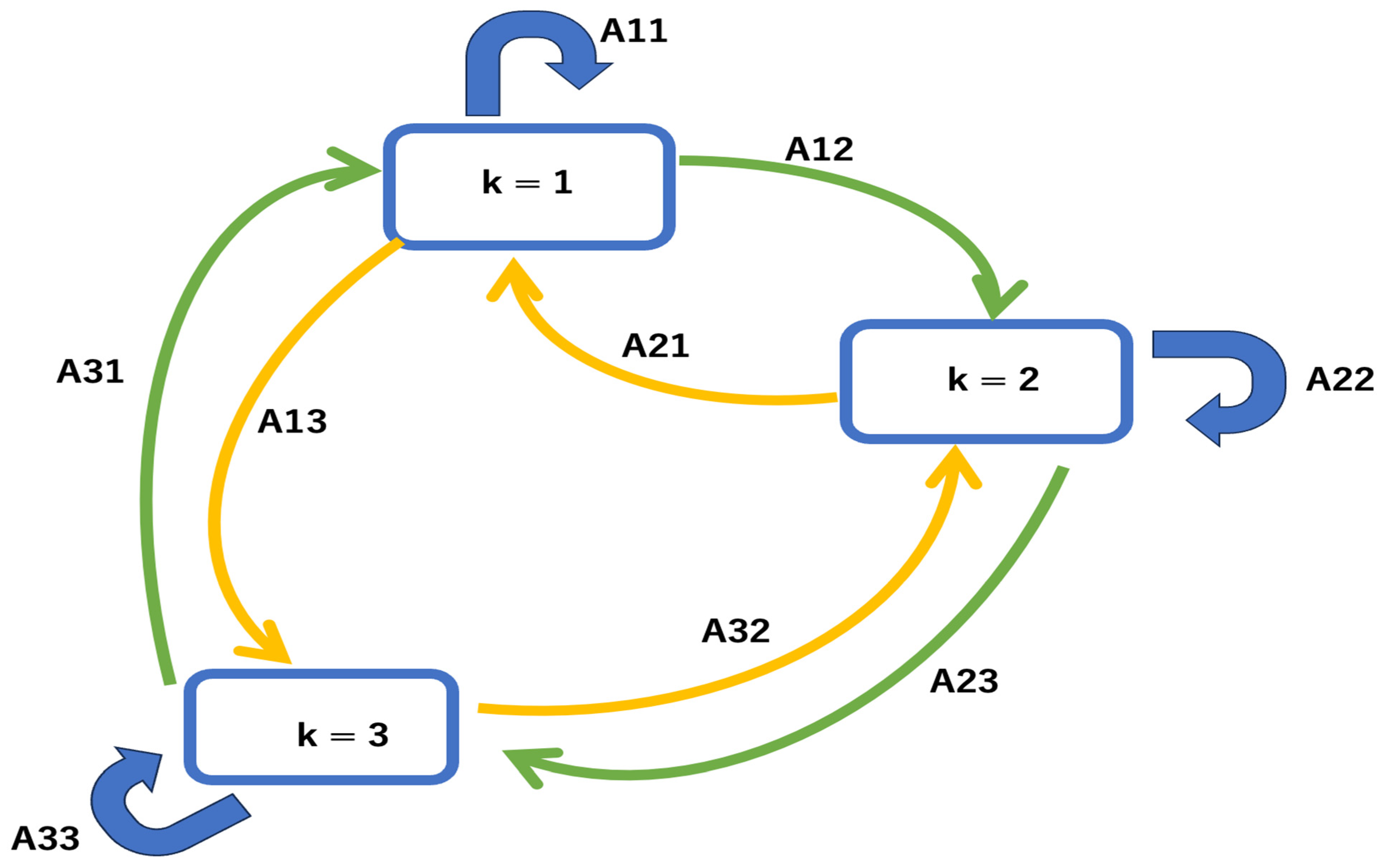
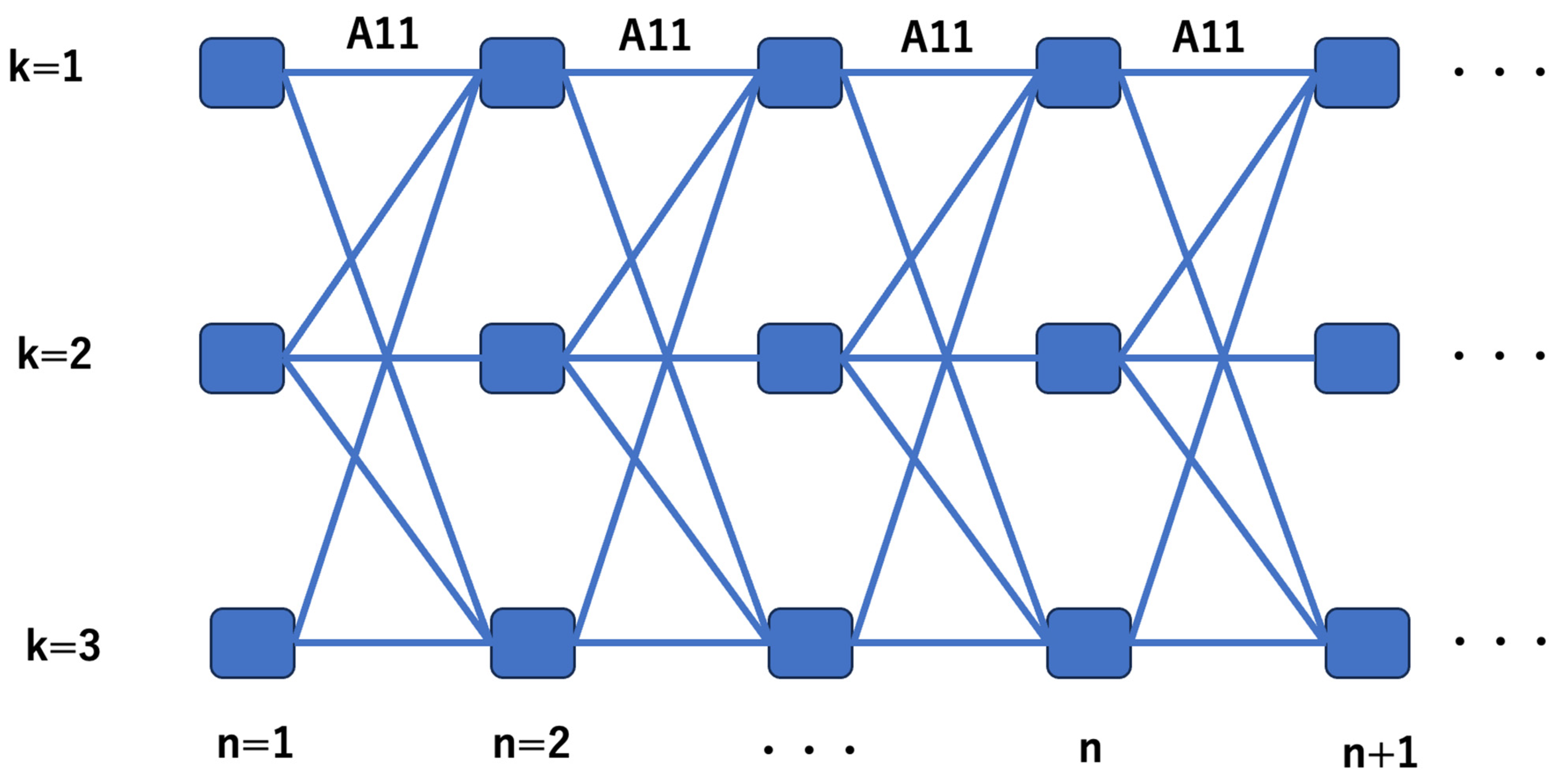
2.2. Modeling of the Biological Immune System

The cells necessary for the model to be constructed include helper T cells (Th cells), killer T cells, antigen-presenting cells, and other immune cells. This model solves rules that do not match patterns using reaction probabilities. The idea is that if a rule that matches any pattern is matched an arbitrary number of times, no pattern matches the pattern [10]. The number of matches is adjusted by the number of antigen presentation rules; however, if there is a pattern match in the first step, the process moves to the second step, which is the matching of TCR and peptide fragments.

Many software systems have been created that are based on the fundamentals of biological phenomena or imitate their mechanisms, i.e., a type of system that mimics the immune system of a living body. The body’s immune system distinguishes between the self and non-self and eliminates the non-self. Software systems incorporating this mechanism are called AISs and are used for problems that require identification and learning, such as identifying and removing computer viruses. In addition, AIS is a computer system inspired by the fundamentals and processes of the biological immune system, and its algorithms use the learning and memory properties of the immune system to solve problems (

Table 1. Models, types of representation, and applications of AIS.

Model or Technique Description	Aspects of the BIS Modeled	Type of Representation Used	Applications
Meta-stable memory immune system for multivariate data analysis	Immune Networks	Real-valued	Data analysis
An immunity clonal strategy algorithm (ICS) to solve multi-objective optimization tasks	Clonal Selection	Real-valued vectors	Optimization
A chaos artificial immune algorithm (CAIF) via integration of chaotic search and CLONALG	Clonal Selection	Real-valued vectors	Optimization
Techno-streams model for detecting an unknown number of evolving clusters in a noisy data stream	Immune Networks	Real-valued	Clustering
An artificial immune system for email classification (AISEC)	Immune Networks	Two-part word vector	Classification
An adaptive clonal selection (ACS) algorithm that suggests some modifications to the CLONALG	Clonal Selection	Real-valued vectors	Optimization
A self-adaptive negative selection algorithm for anomaly detection	Negative Selection	Binary strings, real-valued	Anomaly Detection
An improved clonal selection algorithm based on CLONALG	Clonal Selection Ag-Ab Binding	Binary strings	Machine Learning
An adaptive immune clonal strategy algorithm (AICSA)	Ag-Ab Binding Clonal Selection	Real-valued vectors	Numerical Optimization problems
A fractal immune network model combining the ideas of fractal proteins with immune networks	Immune Networks	Real-valued	Classification, Clustering
A reactive immune network (RIN) for mobile robot learning navigation strategies within unknown environments	Immune Networks	Real-valued	Robots
A real-coded clonal selection algorithm (RCSA) that enables the treatment of real-valued variables for optimization problems	Clonal Selection	Real-valued vectors	Electromagnetic design optimization
A modified algorithm named doptaiNet as an improved version of opt-aiNet to deal with time-varying fitness functions	Immune Networks	Real-valued vector	Optimization
A novel unsupervised fuzzy KMeans (FKM) clustering anomaly detection algorithm based on clonal selection algorithm	Clonal Selection	Numeric characteristic variables	Computer Security
Immunological algorithm for continuous global optimization problems named OPI-IA	Clonal Selection	Binary String	Optimization
An improved version of OPT-IA called Opt–IMMALG	Clonal Selection	Real-code	Optimization
An immune-based network Intrusion detection system (AINIDS)	Immune Networks	Rules	Computer Security
An adaptive clonal algorithm that suggests some modifications to the CLONALG	Clonal Selection, Receptor Editing	Binary strings	Optimization
A hybrid model that combines clonal selection principles and gene expression programming	Clonal Selection	Symbol strings	Data Mining
A modified algorithm of aiNet to solve function optimization problems	Immune Networks	Real-valued vector	Optimization
Artificial immune network classification algorithm (AINC) for fault diagnosis of power transformer	Immune Networks	Real-valued	Classification
A tree-structured artificial immune network (TSAIN) model for data clustering and classification	Immune Networks, Clonal Section	Real-valued	Classification, Clustering
A hybrid artificial immune network that uses swarm learning	Immune Networks	Real-valued	Optimization
A chaos immune network algorithm combining chaos idea with immune network to improve its ability of searching peaks	Immune Networks	Real-valued	Optimization
A feedback negative selection algorithm (FNSA) for anomaly detection	Negative Selection	Real-valued	Anomaly Detection
An artificial immune kernel clustering network (IKCN) for unsupervised image segmentation	Immune Networks	Real-valued, Image feature sets	Clustering
A technique that combines gene expression programming with clonal selection algorithm for system modeling and knowledge discovery	Clonal Selection	Symbol strings, Binary string	System Modeling
A local network neighborhood artificial immune system (LNNAIS) model for data clustering	Immune Networks	Real-valued	Clustering
An improved clonal selection algorithm based on CLONALG with a novel mutation method, self-adaptive chaotic mutation	Clonal Selection	Real-valued	Optimization
A differential immune clonal selection algorithm (DICSA) combining the mechanism of clonal selection and differential evolution	Clonal Selection	Real-valued	Optimization
A novel anomaly detection algorithm based on real-valued negative selection system	Negative Selection	Real-valued vectors	Anomaly Detection
A parallel clonal selection algorithm for solving the graph coloring problem	Clonal Selection	Real-valued	Optimization
A fuzzy artificial immune network (FaiNet) algorithm for lead classification that includes three parts, AIN learning algorithm, MST algorithm, and fuzzy C-means algorithm	Immune Networks	Real-valued vectors	Classification
A clonal chaos adjustment algorithm (CCAA) that improves the search efficiency of CLONALG	Clonal Selection, Immune Networks	Real-valued	Multi-Modal Function Optimization
Artificial negative selection classifier (ANSC) that combines the negative selection algorithm with clonal selection mechanism	Negative Selection, Clonal Selection	Real-valued	Multi-Class Classification

) [11]. AIS began in the 1970s with research on immune networks, but was established as a field in the mid-1990s [12]. Research on negative selection began in 1994, and research on negative selection algorithms has progressed. Initially, AIS attempted to efficiently abstract processes found in the immune system. Recently, there have been attempts to apply AIS to bioinformatics problems and advances in the modeling of biological processes. Some combine AI with some AIS algorithms, which are closely related to genetic algorithms. The processes simulated in AIS include B cell pattern recognition, hypermutation and clonal selection, T cell negative selection, affinity maturation, and immune network theory.

3. Neural Network

A neural network is a mathematical model of artificial intelligence (AI) in which “processing units that linearly transform input” are connected in a network and mimic the network of nerve cells and neurons in the brain. The inputs and outputs of processing units, including linear transformations of inputs, are connected to form a network (

Table 2. Learning tools in deep learning.

Tool	Caffe	Chainer	Theano	Torch7	DL4J
Developer	Univ. of California, Berkeley	Preferred Networks Inc. (Tokyo, Japan)	Univ. de Montral	Facebook, Twitter, Google	Skymind
Language	Python, MATLAB, C/C++	Python	Python	Lua, C/C++	Java, Scala, Clojure, Python, Rudy, etc.
Target	Image	Image, audio, text, etc.	Image, audio, text, etc.	Image, audio, text, etc.	Image, audio, text, etc.
OS	Ubuntu, RHEL/CentOS, OSX	Unspecified	Windows, Ubuntu, CentOS6+, OSV	Ubuntu12+, OSX	Windows, Ubuntu, OSX

) [13]. Each unit must contain a linear transformation of the input and often a nonlinear transformation that follows.

Unit(x) = s(wx)

(1)

Various models have been proposed depending on the configuration of units (e.g., dimensions of linear transformation, presence/absence/type of nonlinear transformation) and network structure (e.g., number of units, hierarchical structure, mutual coupling, recursion of input/output) [14,15,16]. When the weight of the linear transformation (weighting of the input) changes, the output of the neural network also changes, i.e., weight learning is possible. Therefore, neural networks are used as models for machine learning and for various classes of tasks, such as classification, regression, and generation, with or without supervision [17,18,19,20]. Applications include pattern recognition, a type of natural information processing that selects and extracts objects that have certain rules and meanings from data that include miscellaneous information such as images and sounds, data mining, and technology that extracts knowledge by comprehensively applying data evaluation techniques such as statistics, pattern recognition, and AI to large amounts of data (e.g., image recognition, recommendation) [21].

4. Pattern Recognition

Pattern recognition includes techniques such as speech recognition, which recognizes and extracts human voices from voice data and interprets them as commands in optical character recognition (OCR), where characters from image data are recognized and converted into text data and a full-text search system, which recognizes specific keywords and searches documents from a large amount of document information [22,23].

The human brain employs a very natural process for acquiring perceptual and linguistic abilities at the developmental stage of infants and children. However, artificial realization with a computer involves difficulties in terms of accuracy and speed. In recent years, research from the standpoint that “recognition can be reduced to the identification problem of what class it is classified into after all” has been combined with research on AI and statistics to produce great results. As classifiers, non-rule-based methods such as neural networks, support vector machines (SVMs), k-nearest neighbor classifiers, and Bayes classifiers that construct classification parameters from a large amount of data by machine learning are the mainstream approaches [24,25,26]).

4.1. Target Example of Pattern and Speech Recognition

Speech recognition is a function that allows a computer to recognize human voices, etc., and converts spoken words into character strings, or captures the characteristics of voices to identify the person who is speaking. In other words, it refers to a function that converts spoken works into character strings and identifies the person speaking by capturing the characteristics of the voice. The ability to convert spoken words to text is an alternative to keyboard input using the fingers. When only the function of inputting character strings (sentences) is called separately, it is called “voice input” or “dictation (listening)”. It is also possible to operate the application using voice recognition, just as the application can be operated by entering character strings or shortcuts from the keyboard.

Operating an application by voice is called “voice operation” [27]. “Speech recognition” may include the ability to identify the speaker. This is a function that performs personal authentication by comparing voice patterns recorded in advance, and this function is also called “speaker recognition”.

4.2. Recognition Technology

Recognition technology accumulates speech features from training data consisting of recordings of many utterances. It then compares the features extracted from the input speech to be recognized with the accumulated features, and outputs the closest language sequence as the recognition result. In general, the acoustic and linguistic features of speech are often handled separately. Acoustic features represent the frequency characteristics of each phoneme to be recognized and are termed acoustic models. As an acoustic model expression, a hidden Markov model with a mixed normal distribution as the output probability is widely used [28,29,30]. Linguistic features represent restrictions on the arrangement of phonemes and are called language models. As a language model expression, when the language to be recognized is large, n-grams are often used for document creation on a personal computer, and when the language to be recognized is small enough to be covered manually, context-free grammar is used for voice operation, as has been demonstrated in car navigation systems [31,32].

It is an early speech recognition method, but has fallen into disuse as methods based on hidden Markov models have become popular. The Markov model is an algorithm that measures the similarity between two signal sequences that differ in time or speed. For example, the walking pattern of a human being has a certain pattern regardless of whether the person walks quickly or slowly and whether the walking image is fast-forwarded or played back slowly. DTW can be applied not only to audio, but also to any time series data such as video [33]. Speech recognition is used to detect certain patterns regardless of the rate of speech; therefore, standard patterns for comparison are required, and the recognizable vocabulary is limited.

A speech signal can be viewed as a fragmentary or short-term stationary signal to which an HMM can be applied. Thus, the speech signal can be approximately regarded as a stationary process when viewed in a short time of approximately 10 ms. Therefore, speech can be considered a Markov chain of many stochastic processes. In addition, HMM speech recognition is automatically trained, simple, and not very computationally intensive. In the simplest possible setting for speech recognition, the HMM will output a real-valued vector of, for example, 13 dimensions every 10 milliseconds, whose vector consists of cepstrum coefficients, i.e., a signal obtained by treating the frequency spectrum as a signal and performing a Fourier transform [34]. The Fourier evaluation of a time series signal produces a spectrum. Because a Fourier test is performed on the obtained frequency sequence signal, it was named cepstrum using an anagram [35]. The cepstrum coefficients are the first and maximum coefficients of the short-time Fourier transforms of the signal using the cosine transform.

HMMs tend to have probability distributions that are a mixture of Gaussian distributions of diagonal covariances that give the likelihood of each observed vector [36]. Each word and phoneme has its own output distribution. The HMM for a word string is obtained by connecting the HMM for single words or phonemes. There are concepts of speech recognition technology using HMM. Systems with large vocabularies consider contextual dependencies for phonemes. In addition, cepstrum normalization is performed to normalize differences between speakers and recording situations. Other attempts at speaker normalization include vocal tract length normalization (VTLN) for gender normalization and maximum likelihood linear regression (MLLR) for a more unspecified number of speakers [37].

The HMM is a so-called state-space model algorithm that assumes discrete states, and Bayesian estimation is used for learning. The Markov property, which is assumed in HMM, is the property that information at time n is only based on previous information [38]. When considering time series data, the information obtained at time n has properties influenced by information from the past, that is, information from time 1 to n − 1. This data string with a Markov property can be expressed using the probability multiplication theorem. If the data string obtained from time 1 to N is X = {x1, x2, x3, ……, xN}, then the probability distribution representing the obtained data is

$$\begin{array}{ll}\mathrm{p}\left(\mathrm{X}\right)& =\mathrm{p}(\mathrm{x}1,\mathrm{x}2,\mathrm{x}3,\dots \dots ,\mathrm{x}\mathrm{N})\\ & =\mathrm{p}\left(\mathrm{x}1\right)\prod _{\mathrm{n}=2}^{\mathrm{N}}\mathrm{p}\left(\mathrm{x}\mathrm{n}\right|\mathrm{x}1,\dots \dots \dots ,\mathrm{x}\mathrm{n}-1)\end{array}$$

(2)

Furthermore, a model that introduces a process that is strong against the Markov property and in which the data xn obtained at the current time n are only based on the information at the previous time n − 1 is called a first-order Markov property. The Markov property is the assumption that current data are based on all past information. However, assuming a first-order Markov property and because the observed value at n is only affected by the value at time n − 1, the joint probability distribution shown in (1) can be rewritten as follows:

$$\mathrm{p}(\mathrm{x}1,\mathrm{x}2,\mathrm{x}3,\dots \dots ,\mathrm{xN})=\mathrm{p}(\mathrm{x}1){\prod }_{\mathrm{n}=2}^{\mathrm{N}}\mathrm{p}\left(\mathrm{x}\mathrm{n}\right|\mathrm{x}\mathrm{n}-1)$$

(3)

It can also be expressed from the definition of the first-order Markov model:

$$\mathrm{p}\left(\mathrm{x}\mathrm{n}\right|\mathrm{x}1,\mathrm{x}2,\mathrm{x}3,\dots \dots ,\mathrm{xn}-1)=\mathrm{p}(\mathrm{x}\mathrm{n}|\mathrm{x}\mathrm{n}-1)$$

(4)

HMM is a model in which, when there is an observed value, multiple discrete states are hidden behind it and the observed value is caused by those states. For example, when considering a weather forecasting model, a model that predicts whether it will be “sunny”, “cloudy”, or “rainy” daily can also be called HMM. It is easy to imagine this regarding the weather, but when predicting the day’s weather, you can use the previous day’s weather as a reference. In general, if we consider a hidden Markov model where the state K is K = 3, there are three states, and the state transitions to these states as time changes. Also, let the state at n be Zn. Since there are currently K types of states, bmZn is expressed as follows using the 1-to-K encoding method. At time n, when in state k, the k-th element Znk of bmZ becomes 1, and otherwise becomes 0.

Zn = [0, 0, 0, 1, 0, 0]

(5)

$${\sum }_{\mathrm{k}}\mathrm{Z}\mathrm{n}\mathrm{k}=1$$

(6)

Next, regarding the probability p(Zn) of obtaining the state at the current time n in the HMM, the probability model is constructed by considering a transition from a previous state to another state. Now, if we express the probability of being in state j at time n−1 and transitioning to k at the next time n as Ajk, we can draw a state transition diagram like the one below (Figure 3). This is simply a pattern with K = 3, but the state transition of the Markov model can be written using the transition probability Ajk.

Also, Ajk can define the types of K², so these are collectively expressed as a matrix, which is called a transition matrix. If the probability of transitioning from state j at time n − 1 to k at time n is expressed as Ajk, then the following state transition matrix A is defined as follows:

$$\mathrm{A}=\left(\begin{array}{ccc}\mathrm{A}11& \mathrm{A}21& \mathrm{A}31\\ \mathrm{A}12& \mathrm{A}22& \mathrm{A}32\\ \mathrm{A}13& \mathrm{A}23& \mathrm{A}33\end{array}\right)$$

(7)

Here, the transition probability Ajk satisfies the following conditions:

0 ≤ Ajk ≤ 1

(8)

$${\sum }_{\mathrm{k}}\mathrm{A}\mathrm{j}\mathrm{k}=1$$

(9)

Here, p(Zn) depends on the previous state and the probability of this transition; therefore, it can be written as p(Zn|Zn−1, A) using conditional probability, as follows:

$$\mathrm{p}(\mathrm{Zn}|\mathrm{Zn}-1,\mathrm{A})=\prod {\prod }_{\mathrm{k}=1}^{\mathrm{K}}{\prod }_{\mathrm{j}=1}^{\mathrm{K}}{\bigwedge }_{\mathrm{j}\mathrm{k}}^{\mathrm{Z}\mathrm{n}-1,\mathrm{j}^\mathrm{z}\mathrm{n}\mathrm{k}}$$

(10)

Regarding Equation (9), because the initial value cannot be expressed, the initial value is introduced as follows:

$$\mathrm{p}(\mathrm{Zn}|\mathsf{\pi })={\prod }_{\mathrm{k}=1}^{\mathrm{K}}{\mathsf{\pi }}^{{\mathrm{z1k}}_k}$$

(11)

The diagram of the HMM can be expressed as in Figure 4. This is called a trellis diagram.

In addition, the HMM defines the conditional probability distribution p(xn|Zn,φ) of the observed variables.

$$\mathrm{p}(\mathrm{xn}|\mathrm{Zn},\mathsf{\phi })={\prod }_{\mathrm{k}=1}^{\mathrm{K}}{\mathrm{p}\left(\mathrm{x}\mathrm{n}\right|\mathsf{\phi }\mathrm{k})}^{\mathrm{Znk}}$$

(12)

Considering the joint distribution of unobserved state sequence Z and the observed value X in the HMM, the HMM is a model in which the state sequence Z undergoes state transitions according to the Markov model, and the observed value is observed according to equation (10) that relies on the state, which can be described as follows:

p(X, Z|θ) = p(x1, x2, x3, …, xn, z1, z2, z3, …, zN|θ)

(13)

= p(z1|π) p(x1, x2, x3, …, xn, z1, z2, z3, …, zN|θ)

(14)

$$=\mathrm{p}(\mathrm{z}1|\mathsf{\pi }){\prod }_{\mathrm{n}=2}^{\mathrm{N}}\mathrm{p}(\mathrm{z}\mathrm{n}|\mathrm{z}\mathrm{n}-1,\mathrm{A})\mathrm{p}(\mathrm{x}1,\mathrm{x}2,\dots \mathrm{x}\mathrm{n}|\mathrm{z}1,\mathrm{z}2,\dots \mathrm{z}\mathrm{N},\mathsf{\theta })$$

(15)

The reason why it considers the joint distribution of latent variables and observed values, as shown in Equation (13), is that by considering this joint distribution, it is possible to learn parameters in HMM using the EM algorithm.

Thus, the Markov property is a type of property of a stochastic process in probability theory, and the conditional probability distribution of the future state of the process is only based on the current state and does not rely on any past state. That is, given the past state, the current state (the path of the process) is conditionally free. A stochastic process with Markov properties is called a Markov process, and these include the following types:

Markov chain: Among Markov processes, which are a type of stochastic process, this is a Markov process whose possible states are discrete, finite, or countable (discrete-state Markov process). In a Markov chain, future behavior is only affected by current values and is unrelated to past behavior (Markov property). Regarding state changes, or transitions that occur at each time point, a Markov chain is a sequence in which the transition probability does not rely on past states, but only on the current state.

Markov process: This is a stochastic process with a Markov property, which means that future behavior is only affected by current values and is unrelated to past behavior. Such a process can be seen, for example, in the temporal evolution of physical phenomena that can only be described probabilistically. This is because the future behavior of particles is only affected by their current behavior, and this property also carries over to situations where the number of particles in the system increases and requires probabilistic study.

The Markov processes are classified as follows:

Simple Markov process: A Markov process in which the next event is identified from only one state. The term simply Markov process often refers to a simple Markov process.

N-order Markov process: A Markov process in which the next event is identified from a sequence of N consecutive states. Any N-order Markov process can be expressed as a simple Markov process (first-order Markov process) by creating a new state space with N state sets. This is also called an N-fold Markov process.

Discrete-time Markov process: A Markov process in which the time parameter moves through a discrete set. Usually, T = {1,2,3,……} is a set of times.

Continuous-time Markov process: A Markov process whose time set is T = [0, ∞], etc.

Discrete Markov process: A Markov process whose state space is a discrete set. Here, the state space is a space in which a Markov process takes values.

Continuous Markov process: The trajectory of a continuous-time Markov process is continuous in time.

Temporally uniform Markov process: A Markov excess whose transition probability is constant regardless of the current time.

The distribution of a Markov process that normally appears can be determined by the transition probability. The transition probability of the Markov process Xt is the probability P(s, t; x, Y) of leaving point x in the state space at time s and entering the measurable subset Y of the state space at time t > s, defined by the following formula:

$$\mathrm{P}(\mathrm{s},\mathrm{t};\mathrm{x},\mathrm{Y})=\mathrm{P}(\mathrm{Xt}\in \mathrm{Y}|\mathrm{Xs}=\mathrm{x})$$

(16)

In the case of a discrete-time Markov process, the transition probability for t = s + 1 is sufficient, and the transition probability for other periods can be calculated using the Chapman–Kolmogorov equation, as follows:

$$\mathrm{P}(\mathrm{s},\mathrm{u};\mathrm{x},\mathrm{Z})=\int \mathrm{P}\left(\mathrm{t},\mathrm{u};\mathrm{y},\mathrm{Z}\right)\mathrm{P}(\mathrm{s},\mathrm{t};\mathrm{x},\mathrm{d}\mathrm{y})$$

(17)

This is an equation that shows the relationship between the transition probabilities between three times and is given for times s < t < u; that is, the probability of leaving x at times s and entering Z at time u is calculated based on where it is at time t along the way. In addition, the following HMM algorithms are available:

Forward/backward algorithm: This algorithm calculates the probability of each internal state at each step, given the HMM parameters (initial probability, transition matrix, output matrix) and output sequence. The forward algorithms in the context of HMM are used to compute a “belief state”, i.e., the probability of a state at a particular point in time given the history of evidence. This process is also called filtering, and the algorithm is closely related to, but distinct from, the Viterbi algorithm. Forward and backward algorithms seem to be simply names given to a set of standard mathematical procedures within a field; therefore, they need to be placed within the context of probability.

The main observations made by forward and Viterbi algorithms are efficient ways to organize Bayesian updates and inferences in the context of a directed graph of variables. When improving past estimates, backward algorithms complement forward algorithms by considering future history, which is called “smoothing” and is calculated by a forward/backward algorithm. Therefore, a complete forward/backward algorithm considers all evidence. Although the belief state can be computed at each time step, this does not produce the strictly most likely state sequence, but, rather, the most likely state sequence at each time step considering previous history. The Viterbi algorithm is required to obtain the most probable sequence. Forward algorithms are primarily used in applications that define the probability of being in a particular state given a known set of observations. First, the state probability is computed for the previous observation and is used for the current observation.

Next, the transition probability table is used to expand to the next step. This approach essentially caches the probabilities of all intermediate states; therefore, the probabilities of intermediate states are calculated only once, a step that is also called post-decryption. This is useful when calculating fixed-state paths. This algorithm calculates probabilities much more efficiently than naïve approaches that immediately cause a combinatorial explosion. Combining these results gives the probability of a particular emission/observation at each location in the observation set. On the basis of this information, the most likely version of the state path is calculated. This algorithm can be applied anywhere a model can be trained when receiving data using the Baum–Welch algorithm or the general expectation–maximization (EM) algorithm. The forward algorithm then tells us about the probability of the data expected from the model.

Viterbi algorithm: This algorithm is a type of dynamic programming algorithm that searches for the most likely sequence of hidden states (called a Viterbi path) resulting from an observed event sequence, and is specifically based on HMMs. This algorithm estimates the internal state path driving to that state using maximum likelihood, given the HMM parameters (initial probability, transition matrix, output matrix) and output sequence. Forward algorithms, which are algorithms for calculating probabilities of observed event sequences, are also closely related and are part of information theory. This algorithm has several prerequisites. First, observed and hidden events are arranged in one series. This series is often a time series.

There is a one-to-one correspondence between these two sequences, where one observed event corresponds to exactly one hidden event. Third, the calculation of the most likely hidden event at time t is only based on the sequence of observed events at t and the most likely hidden event at t − 1. All of these requirements are satisfied by the first -order HMM. The terms “Viterbi path” and “Viterbi algorithm” are used in reference to a dynamic programming algorithm, which is a method that divides a target problem into multiple subproblems and solves them while recording the calculation results of the subproblems to suppress the number of calculations of the generation probability of each state transition pattern that provides the single most likely explanation for an observation. Based on this idea, the Viterbi algorithm is based on the idea that “for each state, it is only necessary to record the previous state that has the highest cumulative probability.” For example, when focusing on state A in Figure 3, states B and C transition to A (Figure 5). When the product of B’s output probability and state transition probability is greater than that of C, “B” is recorded in the storage area corresponding to state A. By performing this recording for all states, the optimal state transition sequence can finally be determined.

Baum–Welch algorithm: This algorithm is a generalized expectation maximization method (GEM) that estimates the HMM parameters (initial probability, transition matrix, output matrix) using the EM algorithm when the HMM output sequence is given. For the HMM parameter group, the predicted maximum likelihood value, posterior probability, and mode can only be calculated from the output of the training example. Specifically, the probability of an internal state is calculated using a forward/backward algorithm based on the initial parameters, and the parameters are repeatedly updated to make it easier to obtain a given output sequence from the internal state. This algorithm consists of the following two steps:

(1)

For each state of the HMM, forward and backward probabilities are calculated.

(2)

Based on this calculation, the frequency of the values of the transition–output pair is determined and divided by the probability of the entire string. This corresponds to the calculation of the expected number of times for a particular transition–output pair. Each time a specific transition is found, the value of the transition quotient divided by the probability of the entire string increases, and this becomes the new value of the transition.

4.3. Evaluation Index

Word error rate (WER): This is a common indicator of the performance of speech recognition or machine translation systems. A common difficulty in performance measurement lies in the fact that the recognized word sequence may have a different length than the reference word sequence (which is probably correct). WER is derived from Levenshtein distance and operates at the word level rather than the phoneme level. WER is a valuable tool for comparing different systems and evaluating improvements within one system. However, this type of measurement does not provide details about the nature of the translational error, and further work is needed to identify the main sources of error and focus research efforts. This problem is solved by first using dynamic string alignment to align the recognized (spoken) word sequence.

In addition, this problem is investigated through a theory called the power law, which is the correlation between difficulty and WER. A representative corpus for evaluating WER is the WSJ corpus [39]. WER measures how accurately a machine can transcribe what a speaker is saying. Human speech is labeled in the same audio that the machine learning model uses to identify the correct answer for speech-to-text conversion. WER is calculated by dividing the number of incorrectly recognized errors by the total number of words based on the “edit distance”.

For two sentences, the minimum number of operations required to repeat the following three operations on one sentence to match the other is called “edit distance”. (I) Insert: insert a new word between two adjacent words, (II) delete one word, (III) replace: delete one word. WER is the edit distance between the output sentence and the correct sentence (the same as the number of insertions, deletions, and replacements) divided by the number of words in the correct sentence. To calculate the WER, we first add up the number of substituted words, inserted words, and deleted words that occur during the word recognition sequence. The total number is divided by the total number of correct words. Word substitution occurs when words are mixed. Inserting a word occurs when a word is added that is not actually included. Word deletion refers to cases in which words are missing during dictation.

WER = (Number of inserted words + Number of replacement words
+ Number of deleted words)/(Number of correct words)

(18)

A lower WER number indicates that the speech-to-text engine is more accurate (with fewer errors).

Character error rate (CER): The performance of speech recognition models is evaluated using metrics such as WER and CER. WER is the number of incorrect words divided by the number of words in the correct sentence between the speech recognition result and the correct sentence.

However, the CER is similarly calculated on a character-by-character basis. For reference, a WER of 75% or higher is required for a human to be able to understand the meaning of a text when reading it. For practical use as a speech recognition model, the performance is required to be 85% or higher for minutes and 95% or higher for the reading of manuscripts. It is often performed in conjunction with WER evaluation. The CER for the WSJ corpus is below 1% [40].

CER = (Number of inserted characters + Number of replacement characters
+ Number of deleted characters)/(Number of correct characters)

(19)

Phoneme error rate (PER): This refers to the recognized “phoneme” error rate. Texas Instruments and Massachusetts Institute of Technology (TIMIT) is a representative corpus for evaluating PER. The PER against the TIMIT corpus is below 10% [41]).

4.4. Speech Recognition Practices and Issues

Computer usage began to spread after the 1970s, and by the early 21st century, enormous amounts of money and talented human resources had been invested in the research and development of speech recognition systems. Animated films represented by 3D images created by digital technology, as well as the recording and playback of moving images, still images, and music, have become big industries since then, but there is a large difference. A speech recognition system that uses a method called “dictation”, in which pre-training is performed for a limited number of speakers, can achieve an 80% recognition rate in Japanese in an ideal environment [42].

However, 60% is the limit without such training. A system with a limited vocabulary that does not require training can recognize speech from an unspecified number of speakers, but it is limited in its scope of use. The same system was shown to have a 90% recognition rate for Western languages with few homonyms. The speech recognition software commercially available for individuals shows a sufficiently practical recognition rate if the user uses a headset in a quiet room. However, even indoors, it is difficult for the system to accurately recognize speech in an environment where there is a loud conversation in the background or in a noisy environment such as outdoors.

Natural language processing (NLP) is plagued by a lack of data that can be used for learning, but pre-training the language structure can greatly improve the data shortage problem. Because NLP is a diverse field with many different tasks, most tasks require unique datasets; however, these unique datasets contain only a few thousand or hundreds of labeled data. However, modern deep learning-based NLP models show improved quality when trained using millions to billions of labeled datasets. To fill this data gap, general-purpose language representation models are trained and pre-trained, using vast amounts of unlabeled text from the web. Pre-trained models can be fine-tuned for small-scale NLP tasks, such as question answering or sentiment analysis, resulting in significantly higher accuracy than training a model from scratch.

A new technique for pre-training NLP called bidirectional encoder representations (BERT) using transformers builds on recent research in pre-training contextual representations, including semi-supervised sequence learning, generative pre-training, Embeddings from Language Models (ELMo), which is a method for obtaining distributed representations that considers context, and Universal Language Model Fine-Tuning (ULMFit) [43]. However, unlike these previous models, BERT is the first deeply bidirectional unsupervised language representation pre-trained using only a plain text corpus (Wikipedia, in this case).

Pre-trained representations can be either context-free or contextual models, and contextual models can be either unidirectional or bidirectional. Context-free models, such as word2vec and GloVe, ignore context (context-free) and generate embeddings for each word. By contrast, a contextual model generates a model by considering other words in a sentence. However, because BERT is bidirectional, it is expressed using the preceding and following sentences. Beginning at the bottom layer of a deep neural network, it can be performed deeply and interactively. When comparing BERT and other models (OpenAI GPT, ELMo) that use pre-training, the structural feature of BERT is bidirectional, as indicated by the arrow in Figure 6. In contrast, OpenAI GPT uses left-to-right learning, ELMo combines left-to-right and right-to-left learning in the final layer, and only BERT performs bidirectional learning in all layers (Figure 4). BERT’s training consists of two stages: “pre-training” using a large amount of data and “fine-tuning” using a relatively small amount of data. The important point here is that the large amount of data used for “pre-learning” can be ordinary sentences without supervised labels. If plain text is used, it is relatively easy to obtain a large amount of data, such as Wikipedia dumps or newspaper data.

Once “pre-training” is completed using such unlabeled data, a variety of tasks can be handled by “fine-tuning” using a relatively small amount of labeled data based on the pre-trained model. In addition to natural language processing, deep learning models that have grown in scale in recent years require extremely large amounts of training data. For images, it is possible to use large datasets, but this is not the case for natural language processing. The reality is that there are almost no labeled datasets that are sufficiently large to train large-scale models. BERT is a method that can address the issue of the need for large amounts of data, which is inherent in large-scale models, using pre-learning with unlabeled data.

RNNs and CNNs have been used for natural language processing. However, recently, a structure called a transformer has become very popular, and the transformer is also used in the hidden layer of BERT, which inputs a sequence of vectors into the transformer and outputs a sequence of vectors. It has a structure in which multiple transformers are stacked vertically; however, multiple transformers can also be strung together in a daisy chain. BERT performs pre-learning using two objective functions: masked LM and next sentence prediction for input. Thus, in the pre-learning process, BERT evaluates the ability to fill in the blanks in sentences (generating embedded expressions that consider the surrounding context) and has acquired the ability to judge whether two sequences are continuous (the relationship between two sequences).

When attempting to use machine learning to implement natural language processing, which is the process of having a machine understand, distinguish, or generate language, the problem is to create learning data with correct answers. To achieve sufficient accuracy, a considerable amount of data must be prepared, and, in most cases, it is manually created by humans, which requires a considerable amount of time.

To alleviate this problem, a technique called “transfer learning” is often used in machine learning. This method uses two stages of learning: (1) pre-learning and (2) fine- tuning. First, pre-learning involves learning grammar, word meanings, etc., using a large amount of text data available on the Web. This learning method does not require humans to create correct answer data; they only need to collect the data, making it inexpensive. Then, in the fine-tuning stage, data prepared by humans are used for learning. Because the language is learned with basic knowledge of the language already in hand, a small amount of data is required compared to learning from scratch. This is called transfer learning because, what is learned in pre-training is used and transferred to the fine-tuning step. Typical pre-learning methods include those that predict the next word by giving part of a sentence (language model) and those that predict the next word by randomly hiding words in the sentence (denoise).

In addition, ProphetNet performs pre-training similar to a language model. Specifically, when given part of a sentence, instead of only predicting the next word, N words are predicted. The language model predicts the next word for each word, while Bigram ProphetNet predicts the next two words after that. The reason such a method was proposed was because the language model was not able to capture the meaning of the sentence as a whole because it was strongly influenced by the previous word. ProphetNet is designed to enlarge the prediction range and make it easier to see the entire text. Regarding the performance of fine-tuning the pre-trained model for individual tasks, ProphetNet had the highest accuracy when compared with the performance of CNN/Daily Mail and Gigaword for text summarization tasks (

Table 3. Performance of the CNN/Daily Mail test set.

Method	ROUGE-1	ROUGE-2	ROUGE-L
LEAD-3	40.42	17.62	36.67
PTGEN	36.44	15.66	33.42
PTGEN + Coverage	39.53	17.28	36.38
S2S-ELMo	41.56	18.94	38.47
Bottom-up	41.22	18.68	38.34
BERTSUMABS	41.72	19.39	38.76
BERTSUMEXTABS	42.13	19.60	39.18
MASS	42.12	19.50	39.01
UniLM	43.33	20.21	40.51
ProphetNet	43.68	20.64	40.72

and

Table 4. Performance of the Gigaword test set.

Method	ROUGE-1	ROUGE-2	ROUGE-L
OpenNMT	36.73	17.86	33.68
Re3Sum	37.04	19.03	34.46
MASS	38.73	19.71	35.96
UniLM	38.45	19.45	35.75
ProphetNet	39.55	20.27	36.57

).

In addition, because it is assumed to be used at the individual level, the corresponding vocabulary is limited, and business terms are not covered. Furthermore, it is difficult to recognize utterances made by multiple speakers or utterances not intended for speech recognition, such as interviews or meetings. Since the late 2010s, the performance has improved owing to the evolution of AI and deep learning, and it has reached a practical level, such as being used for the voice operation of virtual assistants such as Google Assistant and Amazon Alexa.

However, even people who have received vocal training, such as voice actors, may not be recognized depending on the conditions. On the other hand, for companies, more expensive software is available that can be used to record meeting minutes involving a large vocabulary and multiple speakers. Therefore, efficient work is possible compared to transcription from cassette tapes or IC (integrated circuit) recorders.

4.5. Speech Recognition Technology under Development

If the feature quantity of the speaker’s voice is distorted by noise or feature separation processing, the difference from the acoustic model widens, causing erroneous recognition. The MFT is used in the process of restoring lost speech by estimating how much distortion and noise are included in the feature values of the obtained speech, mapping the reliability on the time axis, and masking low-reliability feature values [44].

Speech recognition based on MFT is an effective method for improving robustness, which detects sub-bands distorted by noise from input speech as missing features [45]. The detected missing features are masked during speech recognition, so that the system is not affected. Therefore, it is possible to respond flexibly, even when the noise changes significantly and dynamically. By applying MFT to the interface between sound source separation and speech recognition, it is possible to improve the accuracy of speech recognition by masking features distorted by sound source separation. Hearing is an important technology for realizing intelligent robots that operate in the same living environment as humans. If a robot hearing system that uses an MFT-based interface between sound source separation and speech recognition is implemented in a humanoid robot to realize robot hearing, high recognition accuracy can be obtained by using a deductive missing feature mask.

The GSS is a technique for separating multiple sound sources [46]. If there is no correlation between sound sources, sound source separation and its position information (sound source localization) can be obtained relatively easily by inputting information from multiple microphones. If this is reflected in the reliability map as noise information of the MFT, the recognition rate will not drop significantly, even in noisy situations or in situations of simultaneous utterances.

The separation performance of GSS, which is a sound source separation method with high separation performance and is suitable for real-time processing, changes depending on the parameter values, and its optimal value varies depending on the surrounding environment, such as the position of the sound source and the noise level [47]. Furthermore, in a dynamic environment, the optimal parameter values change depending on the environment; therefore, it has been difficult to obtain good separation performance with conventional GSS that sets parameters to fixed values. In addition, even in a static environment, there is a problem with the separation performance reaching a plateau due to the GSS algorithm.

To solve the problems associated with the GSS method, which is a sound source separation method suitable for robot hearing, a method was developed that allows for even greater separation performance than conventional GSS by introducing two new processes. One of these processes is the adaptive step size (AS) method for blind source separation (BSS). This makes it possible to adaptively adjust the step size and weighting coefficient, which are important parameters of GSS, according to environmental changes, making it possible to achieve both high separation accuracy and stability. Another process is the optima-controlled recursive average (OCRA) method. This method enables highly accurate correlation matrix estimation without compromising the ability to track environmental changes by using smoothing processing with an exponential window and adaptively adjusting the window length during smoothing according to the degree of separation. By introducing the OCRA, it is possible to improve the separation performance when the GSS converges.

4.6. Practical Examples of Speech Recognition

The speech recognition function on Macintosh was installed in PlainTalk from Quadra 840 AV/Centris 660 AV in 1993. Mac OS9 also has a voice recognition password login function. From MacOS Sierra, Siri, a voice recognition assistant function, was installed, making it possible to perform various operations.

Windows Vista and Windows 7 have a voice recognition function that makes it possible to perform operations such as chatting without keyboard input. There have been several usage methods, such as operating a computer with a voice recognition function. In addition to improving the Japanese recognition rate, Windows operations performed with a mouse and keyboard can be operated by voice. For Windows 10, a voice recognition assistant function called Cortana was installed, and various operations were made possible.

Google Cloud Platform’s Speech-to-Text API makes it easy to integrate real-time speech translation into an application. It supports more than 85 languages and variations, and features accurate speech-to-text conversion using state-of-the-art speech-to-text software. It can be deployed not only in the cloud, but also at the edge, and supports standard and custom voices.

Amazon Alexa is a virtual assistant AI technology developed by Amazon and was first adopted in the smart speaker “Amazon Echo” developed by Amazon Lab126. It can provide real-time information such as voice interaction, music playback, creating to-do lists, setting alarms, streaming podcasts, playing audiobooks, weather, traffic, sports, and other news. Amazon uses the Alexa Voice Service (AVS), a cloud-based service that provides an API to interface with Alexa, to allow device makers to integrate Alexa voice capabilities into their own connected products.

4.7. Optical Character Recognition (OCR)

OCR converts images of printed or handwritten text into strings of character code [48]. The image is captured by an image scanner or photograph, a landscape photograph, or a subtitle in the image. It is widely used as a data entry method for paper-based data, such as passports, bills, bank statements, receipts, business cards, emails, and printed documents that are required for recording in compact form. Furthermore, by converting to character code, it can be used as input for cognitive computing, machine translation, and speech synthesis, and text mining is also possible. The research fields include AI and computer vision, in addition to pattern recognition. Early systems required “training” to read specific typefaces. It is now possible to convert most typefaces with high literacy rates. In some systems, it is possible to produce an output formatted to look like a loaded image. Among them, some are correctly recognized even if parts other than the documents, such as images, are included.

OCR engines have been developed for various domain-specific OCR applications such as receipt OCR, invoice OCR, check OCR, and legal billing document OCR. Examples of these application areas are as follows:

• Data entry from business documents (checks, passports, invoices, bank statements, receipts, etc.);
• Automobile license plate reader (N system);
• Passport recognition and information extraction at airports;
• Automatic insurance document key information extraction;
• Traffic sign recognition systems;
• Extraction of contact information from business card information;
• Rapid creation of text versions of printed documents (e.g., Project Gutenberg book scans);
• Making electronic images of printed documents searchable (e.g., Google Books);
• Recognizing handwritten characters in real time (pen computing);
• Breaking through the CAPTCHA anti-bot system;
• Assistive technology for the visually impaired;
• Instructing vehicles by identifying CAD images in the database that are suitable for real-time-changing vehicle designs;
• Converting scanned documents to searchable PDFs and making them searchable;
• Score OCR to read printed sheet music;
• StotOCR for character recognition of images cut from desktops with screenshots;
• Pre-treatment: OCR software often “pre-processes” images to improve recognition rates;
• Tilt correction: If the document is not aligned correctly when scanned, the document can be tilted clockwise or counterclockwise a few degrees to make the lines of text perfectly horizontal or vertical;
• Speckle removal: Smoothing out contours by removing black and white speckles;
• Binarization: Converting an image from color or grayscale to a black and white binary image. The binarization task is an easy way to separate the desired text or image from the background. Most commercial recognition algorithms only work on binary images; therefore, the task of binarization is essential. In addition, the binarization method should be carefully selected for a particular input image type, because the results of the binarization process greatly affect the quality of the character recognition stage;
• Removing borders: Erasing non-glyph rules and lines;
• Layout analysis, and zoning: Identifying columns, paragraphs, footnotes, etc., as separate blocks, which is especially important in layouts with columns and tables;
• Line and word detection: Establishing a baseline for word and letter shapes, and breaking words as needed;
• Script recognition: In multilingual documents, scripts may change at the word level, requiring script identification before involving the appropriate OCR to process a particular script;
• Aspect ratio and scale normalization: Monospaced font segmentation is achieved relatively simply by aligning the image to a uniform grid based on where vertical grid lines least frequently cross black areas. Proportional fonts require more sophisticated techniques because the whitespace between characters can be larger than the whitespace between words, and vertical lines can intersect multiple characters.

Two basic types of core OCR algorithms produce a ranked list of candidate characters [49] and compare an image to a glyph stored pixel by pixel. This technique is also known as “pattern matching”, “pattern recognition”, and “digital image correlation” [50]. This relies on the input glyphs being correctly separated from the rest of the image and the stored glyphs being of the same font and scale. This method works best when the same type is entered and does not work well when new fonts appear in the middle. This is the technique that early physical photocell-based OCR utilized.

Glyphs are decomposed into “features” such as line segments, closed loops, line directions, and line intersections [51]. The detection function reduces the dimensionality of the representation and makes the recognition process computationally efficient. These features are compared to an abstract vector-like representation of the character and are reduced to one or more glyph prototypes. A common technique of feature detection in computer vision is commonly used in intelligent handwriting recognition and, indeed, most modern OCR software. The nearest neighbor classifier, such as the k-nearest neighbor algorithm, compares image features with stored glyph features and selects the closest match.

OCR can be more accurate if the output only contains words defined in a lexicon, a list of words used in the document. A word list can, for example, define all English words, or more technical vocabulary for a particular domain. This method is difficult to use if the document contains words that are not in the vocabulary, such as proper nouns. Tesseract, which is an optical character recognition engine that runs on various operating systems and has a library for character recognition and a command line interface, uses its dictionary to refine the character segmentation step [52].

The basic output is plain text, but more advanced OCR systems produce an annotated PDF that preserves the original layout of the page and contains both the original image and a searchable text representation. “Neighborhood analysis” takes advantage of the fact that certain words are used together to correct errors. Implementing knowledge about the grammar of the language being scanned, for example, whether a word is a verb or a noun, enables greater accuracy. The Levenshtein distance algorithm is also used in OCR post-processing to further optimize the results from OCR API [53].

The major OCR engines implement OCR systems to process certain types of input more efficiently. In addition to application-specific vocabularies, business rules, standard expressions, and information contained in color images can be used to improve accuracy. This strategy is called “application-oriented OCR” or “customized OCR”, and is used for license plates, invoices, screenshots, ID cards, driver’s licenses, and OCR in the automotive industry.

Full-text search is used to search for a specific character string in multiple documents (files) on a computer. Unlike “file name search” and “character string search in a single file”, it is used in the sense of “searching across multiple documents and targeting the full text contained in the document”. “grep” is a character string search command in UNIX, and searches for character strings to be searched by sequentially scanning the contents of multiple text files. Generally, the search method called “grep type” does not create an index file (index) in advance, but scans the file sequentially, so the search speed decreases as the number of search targets increases.

When the number of documents to be searched is enormous, in the grep type, the documents to be searched increases, and the time required for searching also increases due to accessing each document each time a search is performed and retrieving the relevant data sequentially. Therefore, a method of improving the search performance by scanning a group of documents to be searched in advance and preparing index data that enable high-speed searching has been adopted. Creating an index file in advance is called indexing. The dataset generated by indexing is called an index. The structure is often a list format (table structure) such as “character string/file location/file update data/appearance frequency”. A character string is a search key. By accessing this index at the time of the search, a dramatically higher-speed search becomes possible.

4.8. Index String Extraction Method

In the case of English text, spaces are inserted between words, so index data can be easily created by extracting character strings separated by spaces. However, in the case of Japanese, since there is no custom in which words are separated by spaces, it is necessary to use morphological analysis technology to analyze the context, decompose words, and create an index based on this. A dictionary for analysis is essential for morphological analysis, and the quality of the dictionary influences the search results to some extent. In addition, there are many technical barriers, such as the difficulty in extracting hiragana words that are not registered in dictionaries, and it is said that search omissions occur.

A method of decomposing the search target into characters instead of words and obtaining the frequency of occurrence includes the following N-1 characters [54]. If the value of N is 1, it is called a “unigram”, if it is 2, it is called a “bigram”, and if it is 3, it is called a “trigram”. For example, in the case of the character string “full-text search technology”, if indexing is performed by dividing every two characters into “full text”, “sentence search”, and “technique”, search omissions do not occur and there is no need for a dictionary.

On the other hand, there are two drawbacks compared to morphological analysis. Search results that are different from what was intended (so-called search noise) occur, and the index size bloats. If the search target document is not plain text, for example, an HTML document, it is possible to extract text by removing tags, etc. On the other hand, in the case of a binary format such as the word processor proprietary format of a specific manufacturer, since the indexer cannot extract the text directly from the file, it becomes necessary to use a document filter to extract the text from the file. Some document filter functions are included in indexers, and others are implemented by function extensions such as add-ins.

Indexes for full-text search come in many forms, but the most common is a table with variable-length records, consisting of words and the IDs of the document files containing the words, in an inverted file. Algorithms such as “binary search” that, when searching data in a sorted list or array (assuming no identical values), looking at the central value, using the magnitude relationship with the value to be searched based on a judgment as to whether the value to be searched is on the right or left of the central value, and searching while making sure that it does not exist on one side, can be used for indexing and actual searches to identify document IDs from search words at high speed. The data structure of the inverted file and the search algorithm used vary depending on the full-text search system, and these differences can cause large differences in index size, search speed, and search accuracy.

“Recall” and “precision” are used as one of the evaluation indexes of the full-text search system [55,56]. The former expresses “how few search omissions there are”, and the latter expresses “how little search noise there is”. The retrieval performance of the information retrieval system is commonly used to judge precision and recall mainly from the qualitative viewpoint of accuracy and completeness, and by measuring throughput from the quantitative viewpoint of processing performance. The relevance rate is an index of the accuracy of how many documents matching the search are included in the set obtained as the search result. Also, the recall rate is an index of completeness that indicates how many documents (correct documents) that match the retrieval result among the documents to be retrieved can be retrieved. The precision is as follows:

p = R/N

(20)

(R: the number of retrieved relevant documents, N: the number of retrieved documents). The recall is:

r = R/C

(21)

(R: the number of retrieved relevant documents, C: the number of correct documents among all target documents). If the precision rate is increased, the recall rate will decrease, and if the recall rate is increased, the precision rate tends to decrease, so a scale called F-measure is also often used. The F value is the harmonic mean of precision and recall:

F = 2·p·r/p + r

(22)

= R/1/2 (N + C)

(23)

and corresponds to R divided by the arithmetic mean of N and C. A higher F value means better performance.

The retrieved documents are sorted in “update order”, “file name order”, “document title order”, and the like. Some general search engines also apply their own ranking rules and call them “importance”. The basic concept of ranking is to “display documents that are considered important to the user at the top”. The following methods are often adopted.

• Search word frequency in documents;
• Parsing HTML tags;
• tf-idf: TF indicates the frequency of appearance of a word, and IDF indicates the degree to which words are concentrated in a part of all documents;
• Page rank: Ranking is based on the principle that “pages linked from high-importance pages are important”.

4.9. Computer Vision (CV) for Image Recognition

CV is the field of search that deals with how well computers can understand digital images or moving images. In engineering, it is a field that seeks to automate tasks that the human visual system can perform. Since this field deals with all of the processes in which computers acquire information in the real world, a wide range of research is being conducted, from hardware for image sensing to AI theory for recognizing information. In recent years, the fusion of computer graphics and CV has attracted attention. Research subjects can be broadly classified as follows:

• Image sensor

  -

  Camera,

  -

  Range finder;

• Two-dimensional image processing

  -

  Background subtraction,

  -

  Inter-frame difference method,

  -

  Optical flow,

  -

  Motion vector;

• Three-dimensional image processing

  -

  Stereo method (computer stereo vision),

  -

  Epipolar geometry,

  -

  Shape from X,

  -

  Factorization;

• Recognition/Identification

  -

  Machine learning algorithms (k-nn, k-means, svm, etc.),

  -

  Deep learning algorithms (CNN, RNN, etc.);

• Information presentation

  -

  Virtual reality,

  -

  Mixed reality/augmented reality.

These technologies are deeply connected to robot vision, wearable computers, and so on. In addition, background knowledge such as signal processing and linear algebra is required. Developing a CV to rival the human eye and brain is the problem of an AI-complete, and solving AI-complete computational problems is synonymous with solving the central problem of AI and will create computers as intelligent as humans. The term is analogous to computational complexity theory such as NP-complete problems, where “completeness” in computational complexity theory refers to the most difficult problem in that complexity class [57].

The NP-complete problem is (1) a decision problem (language) belonging to the class NP (non-deterministic polynomial), and (2) any problem belonging to the class NP that can be reduced in polynomial time. Even if the problem definition does not satisfy condition (1), it can be characterized as an NP-hard problem of computational difficulty. Because of the transitivity of polynomial-time reduction, any problem belonging to the class NP that is polynomial-time-reducible from an NP-complete problem is also NP-complete. Most of the proof of NP-complete problems that have been discovered so far was derived from the satisfiability problem and the like due to this transitivity. The satisfiability problem has been proven to be NP-compete, and polynomial-time reduction has shown that many computationally difficult problems are NP-complete. Problems commonly referred to as AI-complete include:

• CV;
• Natural language understanding;
• Passing the Turing test.

4.10. Biometrics (Biometric Authentication or Biometrics Authentication)

Biometrics refers to personal authentication technology and processes that use information on human physical characteristics (biological organs) and behavioral characteristics (habits). In biometric authentication, information called a “template” is collected and registered in advance, and authentication is performed by comparing it with the information acquired by the sensor at the time of authentication [58].

The conditions for biometric information that are suitable for use in biometric authentication include “characteristics that all people have,” “no other person with the same characteristics,” and “characteristics that do not change over time”. It is often used in combination with other biometrics or other authentication methods when it alone does not provide a sufficient and reliable recognition rate.

• Fingerprint

Fingerprints are also used in criminal investigations and are a simple but highly reliable authentication method [59]. In addition, since biometric authentication is one of the oldest methods, many deception methods have been devised, and authentication equipment for these methods has been improved.

• DNA

DNA is often used in criminal investigations as a DNA-type appraisal and is the most reliable and ultimate means of biometric authentication. For confirmation, it is necessary to obtain a sample (a part of the subject’s body such as blood or saliva) and perform a detailed chemical analysis, but no real-time authentication device has been developed. It has the disadvantage that identical twins cannot be distinguished.

• Hand shape

This is a method of authentication using the width of the palm and the length of the fingers. The recognition rate declines with growth and aging, so regular renewal is required (widely used in the US, valid for one year).

• Retina

This is a method of recognizing the pattern of capillaries in the retina of the eye. Since the retina is in the back of the eyeball, it is necessary to bring the eye close to the sensor to photograph the pattern, and the device is large-scale, so the penetration rate is not very high.

• Iris

This authentication method uses a histogram of iris pattern gradation values. Accurate authentication is possible even for twins, so it has high authentication accuracy. Like the retina, large-scale equipment was required in the past, and the registration and operation costs tended to be higher than authentication methods such as fingerprints and veins.

• Face

The recognition rate declines using this method due to eyeglasses, facial expressions, and changes due to aging. Also, in the case of identical twins, it is easy to recognize them as the same person. It is used as a simple authentication method and for criminal investigations.

• Blood vessels

Techniques using vein patterns obtained by transmitting or reflecting near-infrared light to the palm, the back of the hand, and the fingers have been put to practical use.

• Audio

Audio information is derived from the structure of vocal organs such as the vocal cords and is a physical feature, but it also has elements of behavioral features. A technique using a voiceprint is well known, but the recognition rate may decrease depending on the user’s health condition.

• Ear shape

A method of authentication using the shape of the auricle.

• Body odor

A method of authentication based on the chemical composition of body odor.

• Handwriting

A method that uses habits such as changes in writing trajectory, speed, and writing pressure. Research is also being conducted on authentication methods that estimate wrist rotation and finger length. Note that the method of viewing only the handwriting image after writing is not considered biometric authentication.

• Lip movement

A method using the habits of lip movements during speech.

• Blinking

A method for measuring the amount of change in the iris area due to blinking. The unconscious blinking action is fast, and it is difficult for others to imitate it.

• Walking

An authentication method using human walking. Walking has physical characteristics such as bone structure and muscles, and dynamic characteristics such as walking style, and is used in combination with the face recognition system of surveillance cameras. The recognition rate decreases when a person has suffered a serious injury such as a bone fracture or has been hospitalized for a long period.

4.11. Gesture Recognition

Gesture recognition is a subject of computer science and language technology aimed at interpreting human gestures via mathematical algorithms [60,61]. Gestures can originate from any body movement or state, but usually originate from the face and hands. Current focuses in this area include facial emotion recognition and hand gesture recognition. Users can use simple gestures to control or interact with the device without physically touching it. While many approaches have been taken using cameras and CV algorithms to interpret sign language, gesture recognition can be used to understand human language. Therefore, it creates a richer bridge between machines and humans than primitive textual user interfaces or GUIs (graphical user interfaces), which limit keyboard input to a large extent.

4.12. Sign Language Recognition

Sign language recognition can be divided into two types. The first is the method of acquiring hand motions [62,63] and recognizing them by comparing the detected motion pattern with the motion pattern registered in a dictionary. The second is to detect the motion of the hand using a video camera and image processing methods.

4.13. Sketch Recognition

Sketch recognition is the automatic recognition of a diagram by a computer [64]. Sketch recognition research is located at the intersection of AI and human–computer interaction. Recognition algorithms are typically gesture-based, appearance-based, geometry-based, or a combination thereof.

5. Data Mining

Data mining, on the other hand, is defined as “the extraction of information from data that has not been explicitly stated and hitherto unknown, but which is potentially useful and non-obvious,” and a “technical system for extracting useful information from huge data collections and databases”. It often implies the expectation that heuristic knowledge acquisition is possible, which is difficult to imagine from ordinary data handling. Targeting text is called text mining, and targeting web pages is called web mining.

Neural networks with three or more layers have been proven to be differentiable and capable of approximating continuous functions (they can solve linearly non-separable problems).

It is possible to identify characteristic patterns that occur frequently in a dataset.

• Association rule extraction: A technology that extracts events that frequently occur at the same times as highly correlated events, or association rules, from a large amount of data stored in a database;
• Other frequent patterns;
• Time series and graphs.

Classification is the problem of predicting the category corresponding to given data. Typical methods include naïve Bayes classifier [65], decision tree [66], and SVM.

Typical methods used to address the problem of predicting real values corresponding to given data are linear regression [67], logistic regression [68], and SVM.

Some types of data analysis (especially the multivariate analysis method) are unsupervised data classification methods, that is, methods of automatically classifying the given data without external criteria [69].

6. Modeling and Optimization

Machine learning is used in various fields because it can predict and optimize numerical values based on input data if appropriate processing is performed. Loss, also called cost, is the difference between the model’s prediction and the result. Minimizing the value of the loss achieves the optimization of the machine learning model [70]. Therefore, if the prediction value of the neural network changes, the loss will also change.

The predicted value of the neural network varies with parameters, weights, and biases. In other words, to reduce this loss, the values of the parameters in it are adjusted variously so that the neural network produces the correct value. The parameters are the weights and biases of the neural network, which are w and b in the formula below. A is an arbitrary activation function.

y = a (w x + b)

(24)

Since the loss is the difference between the predicted value and the correct value, the loss for one datum is as follows:

Loss = (y − ŷ)² = (y – 1/1 + e^{−w x})²

(25)

where y and ŷ are the correct value and the value predicted by the neural network, respectively. The reason for squaring is simply to make the sign of the loss positive. This squared error is called mean squared error.

The loss function is set according to the situation, such as the “sum of squared error” or “cross entropy error”. Since a neural network produces an output for an input, the neural network is defined as the function f. Since the predicted value ŷ is the output of the neural network f for the input data x, it can be expressed as ŷ = f(x). By manipulating w so that this loss function takes the minimum value, the result is a neural network with the highest parameter w. In other words, it is important to find parameters that minimize the loss function.

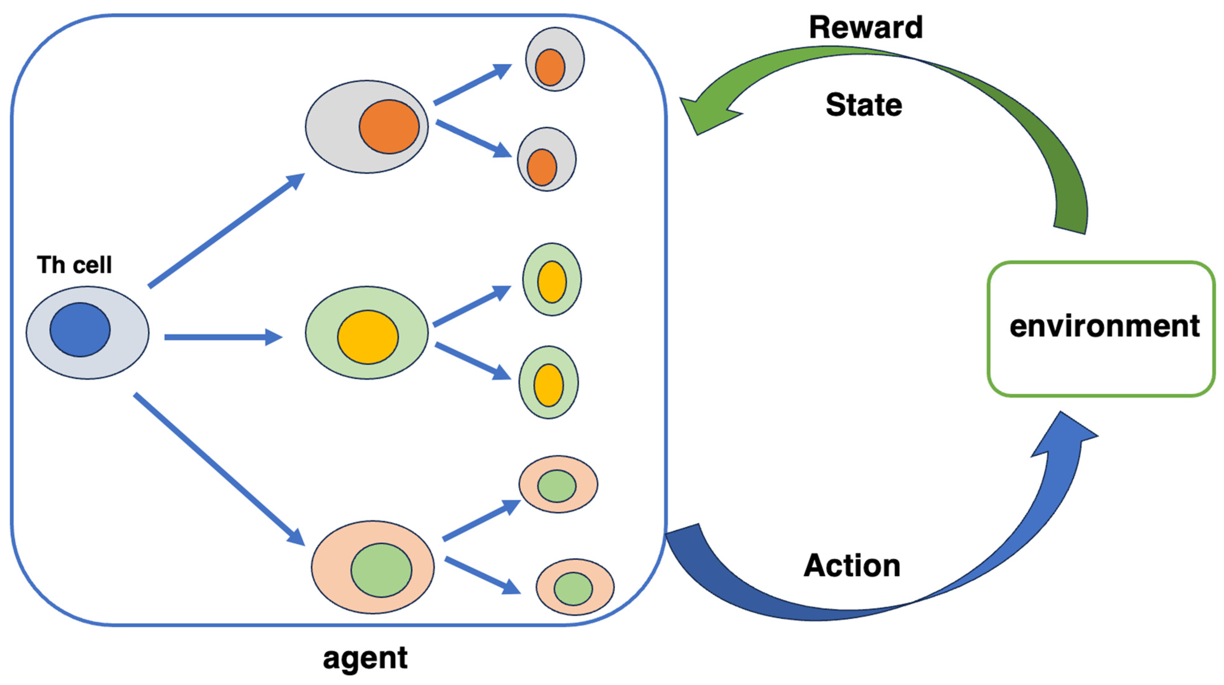
6.1. T Cell Networks and Reinforcement Learning

Living organisms, as represented by the brain, have extremely sophisticated information processing mechanisms that have not yet been realized. The immune system, which protects our bodies by learning about unknown pathogens from past infection history and inducing appropriate responses, is also a biological information processing mechanism. To understand and predict the behavior of a complex learning system, it is not enough to simply enumerate its components and their behavior; a theoretical method that understands the operating principle of the entire system is required.

However, although various cells and molecules related to immunity have been experimentally discovered, the development of comprehensive theories on how these aggregates learn about foreign enemies and mount appropriate immune responses has lagged far behind. By applying the theory of reinforcement learning, which is rapidly developing in the field of AI, a new theory has been constructed that comprehensively deals with the process by which the immune system learns from past infection experiences [71].

The Th cell group, which is an immune cell group responsible for immune memory and learning, is a group of cells that have extremely diverse chemical molecule receptors and sensors. This flow of a “molecular pattern” to the “Th cell group” and then to “another immune cell group” is like the structure of a multilayer neural network. Based on this theory, clonal selection, which is classically known in immunology, is a mechanism by which immune learning is realized by increasing the number of immune cells that contribute to immune recognition in the body and decreasing the number of cells that do not contribute, and can be regarded as a type of learning rule for reinforcement learning (Figure 7). This theory also reproduces the experimentally measured properties of the population distribution of immune cells. In other words, this is a theory that treats immune recognition and control by Th cell groups as a reinforcement learning theory by applying the theory of reinforcement learning using neural networks that have been developed in the field of AI.

Clonal selection is classically accepted as a mechanism by which Th cell populations can remember past infectious agents and a concept that explains pathogen memory and rapid response upon second infection. This a necessary and unnecessary mechanism, and among T cell groups with diverse receptors, the number of cells involved in pathogen recognition increases, and the number of cells that do not participate decreases. The learning rules necessary for realizing learning in the immune system were derived based on the theory of reinforcement learning described above, and learning rules that included clone selection in special cases were derived.

The learning rules were also general, including feedback from other immune cells that activate Th cells and global signals that act on the entire Th cell population, indicating that its existence is experimentally known but is not explained by clonal selection. The shape of the population distribution of Th cell groups learned based on this learning rule closely reproduces the power law properties observed in recent experimental measurements. The immune system, like the brain, is a complex learning system in living organisms, and to predict and control immune behavior, it is necessary to understand the learning process and laws of learning. Although this theory focuses on the Th cell group within the immune system, various other cell groups, including the innate immune system, play different roles in the immune system. Many of these can be understood from the perspective of learning theory. Developing the theory of this research based on reinforcement learning provides a comprehensive understanding of the logic and principles by which the immune system distinguishes foreign enemies from its cells and establishes learning. Combining this kind of theory with quantitative measurements is also expected to greatly expand the possibilities for predicting and controlling the immune system.

6.2. Automatic Tracking of Immune Cells with Deep Learning

Human immune cells are videotaped and their activity levels analyzed using video data, and immunity can be estimated by analyzing the activity levels. Leukocytes are migratory cells that move within tissues using protrusions called pseudopodia, which are responsible for cell movement, and move while changing their shape like an amoeba. Furthermore, leukocytes remove unnecessary cells and malignant cells from body tissues and transmit their antigen information to other immune cells. Because these roles maintain human immune function, leukocytes are important cells that contribute to human health. Therefore, high throughput is required for immune cell analysis, as the amount of activity is analyzed by visually tracking immune cells in body tissue videos. This requires obtaining the initial positions of immune cells in the video and continuously tracking them.

Additionally, the ability to track multiple immune cells simultaneously from a single video can further improve efficiency. One method to achieve automatic tracking is to use deep learning to automatically specify and automatically track multiple immune cells for analysis [72]. The process of this automatic acquisition method consists of two steps: the automatic acquisition of immune cells and the automatic tracking of them. First, a patch image is cut out from the initial frame image of a body tissue video using a search frame with a fixed ratio. A classifier trained by deep learning then identifies whether the extracted patch image is an immune cell or not. Based on the output of the classifier, it is determined whether immune cells are recognized, and if recognized, the position of the search frame is recorded.

To confirm frequently recognized positions, the recognition frequency space has the same vertical and horizontal size as the frame image size, and the height represents the recognition frequency, which can be visualized by adding the bivariate normal distribution values, indicating that immune cells are more likely to be captured the closer they are to the center within the recognized area of the locations corresponding to the recognized positions in the frame image. In addition, a threshold is set in the heat map image of the recognition frequency space to find the center of gravity of each closed region in the binarized image. Currently, the threshold value is lowered in order from the highest frequency value until the number of closed regions reaches the specified number; then, the center of gravity of each closed region is set as the center of gravity of the immune cell and the position of the immune cell is specified.

In addition, automatic tracking focuses on the location in the frame image of the second frame that corresponds to the part where the immune cell position was obtained in the previous frame. Then, the center of gravity of the location recognized as an immune cell in each scanned region is calculated as the position of the immune cell in the second frame. By performing this process, shifting one frame at a time, the movement of the immune cells can be captured sequentially. This classifier solves problems that hinder learning, such as degradation problems, by using shortcut connections that transmit identity maps to various parts of the network in ResNet. In addition, the accuracy can be improved by performing regularization after combining the shortcut and the base network before the convolution layer in the base network to make the shortcut a complete identity mapping step. In this shortcut connection, the identity mapping of the output of the previous layer is added to the input of the layer several layers ahead, so the baseline network parallel to the shortcut only learns the difference before and after the shortcut. When the base network parallel to the shortcut is f (x, W) and the input of the N layer is xn, the input of the L layer is expressed by Equation (7) using the input of the l layer. However, in this case, l < L.

$$\mathrm{x}\mathrm{L}=\mathrm{x}\mathrm{l}+{\sum }_{\mathrm{i}=\mathrm{l}}^{\mathrm{L}-1}\mathrm{F}(\mathrm{x}\mathrm{i},\mathrm{W}\mathrm{i})$$

(26)

The loss function is currently E, and the slope of the loss is calculated by partial differentiation with respect to xl, which is shown in Equation (8). Here, it is said that $1+\partial /\partial \mathrm{x}1{\sum }_{\mathrm{i}=\mathrm{l}}^{\mathrm{L}-1}\mathrm{F}(\mathrm{x}\mathrm{i},\mathrm{W}\mathrm{i})$ almost never becomes 0, so the gradient never becomes 0 and the learning becomes stable.

$$\frac{\partial \mathrm{E}}{\partial \mathrm{x}1}=\left(\frac{\partial \mathrm{E}}{\partial \mathrm{x}\mathrm{L}}\right)\left(\frac{\partial \mathrm{x}\mathrm{L}}{\partial \mathrm{x}\mathrm{l}}\right)=\frac{\partial \mathrm{E}}{\partial \mathrm{x}\mathrm{L}}(1+\partial /\partial \mathrm{x}1{\sum }_{\mathrm{i}=\mathrm{l}}^{\mathrm{L}-1}\mathrm{F}\left(\mathrm{x}\mathrm{i},\mathrm{W}\mathrm{i}\right))$$

(27)

7. Discussion and Conclusions

AI has been applied to many fields, including medicine [73]. Based on a wealth of clinical data, machine learning-adapted medical devices can be expected to help avoid the need for new clinical trials and respond to areas such as regulations and recalls. Further, its performance has surpassed that of humans in resolving several real-world problems, but there are still safety issues such as vulnerabilities and privacy violations. There is a need to build safe, stable, and secure AI models by using CI technologies, including evolutionary calculations, fuzzy systems, and neutral networks.

Specifically, at the model construction and learning stage, evolutionary computation is used to generate adversarial samples that add small amounts of noise that humans cannot perceive to training samples, and these samples are used to generate highly robust AI models. At the same time, optimizing lightweight models that simplify the structure and reduce the amount of calculation without degrading the performance of the AI model is an important issue. In addition, at the stage after the AI model is introduced, it automatically detects vulnerabilities and retrains in a way that can be applied to the trained AI model, and develops a general-purpose framework that could self-evolve and adapt to a variety of new scenarios, which is also an important challenge.

CI systems are defined as those that process low-level data such as numerical data, have a pattern recognition component, and do not use AI knowledge. Additionally, as it begins to exhibit adaptive computing power, fault tolerance, speeds approaching human-like turnaround, and error rates approaching human performance, a clear distinction is made between CI and AI, with AI being based on hard computing techniques, while CI is based on soft computing techniques. AI and CI aim at similar long-term goals, that is, to reach general intelligence: the intelligence of a machine that can perform any intellectual task that a human can perform.

There is a clear difference between these approaches, as CI is a subset of AI. There are two types of machine intelligence: AI, which is based on hard computing techniques, and CI, which is based on soft computing techniques that allow adaptation to many situations. Hard computing technology operates according to binary logic based on only two values (Boolean true or false, 0 or 1), on which modern computers are based. One problem with this logic is that natural language cannot always be easily translated into an absolute term of 0 and 1. This is where soft computing techniques based on fuzzy logic come in handy. This logic is very similar to how the human brain aggregates data into partial truths (sharp/fuzzy systems) and is one of the key proprietary aspects of CI.

Within the same principles of fuzzy logic and binary logic, crispy systems and fuzzy system follow. While crispy logic is part of the principles of AI and consists of the inclusion or exclusion of elements within a set, the fuzzy system allows elements to be partially included in a set. Following this logic, each element can be given a degree of membership, but it is not restricted to one of these two values.

Fuzzy logic, one of the key principles of CI, consists of measurements and process modeling performed using complex real-world processes. In contrast to AI, which requires precise knowledge, process models can face imperfections and, most importantly, data ignorance. This technology tends to be applied in a wide range of fields such as control, image processing, and decision making. Fuzzy logic is primarily useful for approximate reasoning, but it lacks the learning ability required by humans in order to learn from past mistakes and improve yourself. This is why CI experts are working on developing artificial neural networks, which are defined by the following process: a cell body processes information and is then incorporated into distributed information processing systems to enable processing and learning from empirical data, based on biological networks.

From an application perspective, neural networks can be classified into five groups: data analysis, classification, associative memory, pattern clustering generation, and control. Generally, the purpose of this method is to deal with the nonlinearity of the system to control it. Additionally, neural network technology has the advantage of allowing data clustering through fuzzy logic techniques. In addition, evolutionary calculations based on the process of natural selection utilize the power of natural evolution to drive new artificial evolution methodologies. This also includes other areas such as evolutionary strategies and evolutionary algorithms that are considered problem-solving tools. The main application areas of this principle cover areas where traditional mathematical methods are inadequate, such as optimization and multi-objective optimization.

Theoretical learning is one of the main approaches in CI and continues to search for methods of inference that are like humans. In psychology, learning is the process of integrating cognitive, emotional, and environmental influences and experiences to acquire, enhance, or change knowledge, skills, values, and worldviews. Learning theories help us to understand how these influences and experiences are processed and make predictions based on previous experience. Probabilistic methods, one of the key elements of fuzzy logic, were introduced with the aim of evaluating the results of intelligent computational systems that are primarily defined by randomness. Therefore, probabilistic methods derive possible solutions to a problem based on prior knowledge.

CI is the ability to build models based on various phenomena and the data obtained from them using computational means. CI technology includes not only model construction, but also technology to solve various problems by applying a range of computational methods. With the aim of developing CI technology that excels both academically and practically, various benchmark problems are being developed that reflect the difficulty of real-world problems in a wide range of fields. Preparing such benchmark problems is not only helpful in academic aspects such as the optimal combination of machine learning and optimization calculation, but also in the field itself. Therefore, it is expected that CI technology that can be immediately put into practical use for problem solving in the future can be developed.

In addition, by applying the theory of reinforcement learning, which is rapidly developing in the field of AI, it is possible to construct a new theory that deals with the process by which the immune system learns from past infection experiences. It is hoped that this will lead to the development of a theoretical foundation that understands the immune system as a biological learning system like the brain and encompasses and predicts its complex and non-intuitive behavior.

References

- Badura, P.; Pietka, E. Soft computing approach to 3D lung nodule segmentation in CT. Comput. Biol. Med. 2014, 53, 230–243. [Google Scholar] [CrossRef]
- Green, D.; Lavesson, N. Chaos theory and artificial intelligence may provide insights on disability outcomes. Dev. Med. Child. Neurol. 2019, 61, 1120. [Google Scholar] [CrossRef]
- Wang, Z.; Tang, X.; Liu, H.; Peng, L. Artificial immune intelligence-inspired dynamic real-time computer forensics model. Math. Biosci. Eng. 2020, 17, 7221–7233. [Google Scholar] [CrossRef]
- Alghamdi, M.; Maray, M.; Alazzam, M.B. Diagnosis of Breast Cancer Using Computational Intelligence Models and IoT Applications. Comput. Intell. Neurosci. 2022, 2022, 2143510. [Google Scholar] [CrossRef]
- Matarneh, F.M.; Alqaralleh, B.A.Y.; Aldhaban, F.; AlQaralleh, E.A.; Kumar, A.; Gupta, D.; Joshi, G.P. Swarm Intelligence with Adaptive Neuro-Fuzzy Inference System-Based Routing Protocol for Clustered Wireless Sensor Networks. Comput. Intell. Neurosci. 2022, 2022, 7940895. [Google Scholar] [CrossRef]
- Chetty, M.; Hallinan, J.; Ruz, G.A.; Wipat, A. Computational intelligence and machine learning in bioinformatics and computational biology. Biosystems 2022, 222, 104792. [Google Scholar] [CrossRef]
- Zheng, P.; Dou, Y.; Wang, Q. Immune response and treatment targets of chronic hepatitis B virus infection: Innate and adaptive immunity. Front. Cell Infect Microbiol. 2023, 13, 1206720. [Google Scholar] [CrossRef]
- Martins, Y.C.; Ribeiro-Gomes, F.L.; Daniel-Ribeiro, C.T. A short history of innate immunity. Mem. Inst. Oswaldo. Cruz. 2023, 118, e230023. [Google Scholar] [CrossRef]
- Zhang, H.; Gao, J.; Tang, Y.; Jin, T.; Tao, J. Inflammasomes cross-talk with lymphocytes to connect the innate and adaptive immune response. J. Adv. Res. 2023, 54, 181–193. [Google Scholar] [CrossRef]
- Yang, H.; Li, T.; Hu, X.; Wang, F.; Zou, Y. A survey of artificial immune system based intrusion detection. Sci. World J. 2014, 2014, 156790. [Google Scholar] [CrossRef]
- Al-Enezi, J.R.; Abbod, M.F.; Alsharhan, S. Artificial Immune Systems—Models, Algorithms and Applications. IJRRAS 2010, 3, 118–131. [Google Scholar]
- Kephart, J.O. A biologically inspired immune system for computers. In Artificial Life IV: The Fourth International Workshop on the Synthesis and Simulation of Living Systems; MIT Press: Cambridge, MA, USA, 1994; pp. 130–139. [Google Scholar]
- Peng, X.; Feng, J.; Zhou, J.T.; Lei, Y.; Yan, S. Deep Subspace Clustering. IEEE Trans. Neural Netw. Learn. Syst. 2020, 31, 5509–5521. [Google Scholar] [CrossRef]
- Itoh, K.; Miwa, H.; Takanobu, H.; Takanishi, A. Application of neural network to humanoid robots-development of co-associative memory model. Neural Netw. 2005, 18, 666–673. [Google Scholar] [CrossRef]
- Jordanou, J.P.; Antonelo, E.A.; Camponogara, E. Echo State Networks for Practical Nonlinear Model Predictive Control of Unknown Dynamic Systems. IEEE Trans. Neural Netw. Learn. Syst. 2022, 33, 2615–2629. [Google Scholar] [CrossRef]
- Peng, W.; Varanka, T.; Mostafa, A.; Shi, H.; Zhao, G. Hyperbolic Deep Neural Networks: A Survey. IEEE Trans. Pattern Anal. Mach Intell. 2022, 44, 10023–10044. [Google Scholar] [CrossRef]
- Renganathan, V. Overview of artificial neural network models in the biomedical domain. Bratisl. Lek. Listy. 2019, 120, 536–540. [Google Scholar] [CrossRef]
- Zhang, Y.; Lin, H.; Yang, Z.; Wang, J.; Sun, Y.; Xu, B.; Zhao, Z. Neural network-based approaches for biomedical relation classification: A review. J. Biomed. Inform. 2019, 99, 103294. [Google Scholar] [CrossRef]
- Wang, X.; Lin, X.; Dang, X. Supervised learning in spiking neural networks: A review of algorithms and evaluations. Neural Netw. 2020, 125, 258–280. [Google Scholar] [CrossRef]
- Behler, J. Four Generations of High-Dimensional Neural Network Potentials. Chem. Rev. 2021, 121, 10037–10072. [Google Scholar] [CrossRef]
- Shamir, L.; Delaney, J.D.; Orlov, N.; Eckley, D.M.; Goldberg, I.G. Pattern recognition software and techniques for biological image analysis. PLoS Comput. Biol. 2010, 6, e1000974. [Google Scholar] [CrossRef]
- Partila, P.; Voznak, M.; Tovarek, J. Pattern Recognition Methods and Features Selection for Speech Emotion Recognition System. Sci. World J. 2015, 2015, 573068. [Google Scholar] [CrossRef]
- Dinges, L.; Al-Hamadi, A.; Elzobi, M.; El-Etriby, S. Synthesis of Common Arabic Handwritings to Aid Optical Character Recognition Research. Sensors 2016, 16, 346. [Google Scholar] [CrossRef] [PubMed]
- Ho, S.Y.; Hsieh, C.H.; Chen, H.M.; Huang, H.L. Interpretable gene expression classifier with an accurate and compact fuzzy rule base for microarray data analysis. Biosystems 2006, 85, 165–176. [Google Scholar] [CrossRef] [PubMed]
- He, T.; Wang, T.; Abbey, R.; Griffin, J. High-Performance Support Vector Machines and Its Applications. arXiv 2019, arXiv:1905.00331v1. [Google Scholar]
- Gil-Herrera, E.; Aden-Buie, G.; Yalcin, A.; Tsalatsanis, A.; Barnes, L.E.; Djulbegovic, B. Rough set theory based prognostic classification models for hospice referral. BMC Med. Inform. Decis. Mak. 2015, 15, 98. [Google Scholar] [CrossRef]
- Buss, E.; Miller, M.K.; Leibold, L.J. Maturation of Speech-in-Speech Recognition for Whispered and Voiced Speech. J. Speech Lang. Hear Res. 2022, 65, 3117–3128. [Google Scholar] [CrossRef] [PubMed]
- Lee, L.M.; Jean, F.R. High-order hidden Markov model for piecewise linear processes and applications to speech recognition. J. Acoust. Soc. Am. 2016, 140, EL204. [Google Scholar] [CrossRef] [PubMed]
- Moreira, B.S.; Perkusich, A.; Luiz, S.O.D. An Acoustic Sensing Gesture Recognition System Design Based on a Hidden Markov Model. Sensors 2020, 20, 4803. [Google Scholar] [CrossRef] [PubMed]
- You, H.; Byun, S.H.; Choo, Y. Underwater Acoustic Signal Detection Using Calibrated Hidden Markov Model with Multiple Measurements. Sensors 2022, 22, 5088. [Google Scholar] [CrossRef]
- Rohrmeier, M.; Fu, Q.; Dienes, Z. Implicit learning of recursive context-free grammars. PLoS ONE 2012, 7, e45885. [Google Scholar] [CrossRef]
- Ríos-Toledo, G.; Posadas-Durán, J.P.F.; Sidorov, G.; Castro-Sánchez, N.A. Detection of changes in literary writing style using N-grams as style markers and supervised machine learning. PLoS ONE 2022, 17, e0267590. [Google Scholar] [CrossRef]
- Yu, X.; Xiong, S. A Dynamic Time Warping Based Algorithm to Evaluate Kinect-Enabled Home-Based Physical Rehabilitation Exercises for Older People. Sensors 2019, 19, 2882. [Google Scholar] [CrossRef]
- Polur, P.D.; Miller, G.E. Experiments with fast Fourier transform, linear predictive and cepstral coefficients in dysarthric speech recognition algorithms using hidden Markov Model. IEEE Trans. Neural Syst. Rehabil. Eng. 2005, 13, 558–561. [Google Scholar] [CrossRef]
- Chen, X.; Zhu, X.; Zhang, D. Use of the discriminant Fourier-derived cepstrum with feature-level post-processing for surface electromyographic signal classification. Physiol. Meas. 2009, 30, 1399–1413. [Google Scholar] [CrossRef]
- Ezaki, T.; Himeno, Y.; Watanabe, T.; Masuda, N. Modelling state-transition dynamics in resting-state brain signals by the hidden Markov and Gaussian mixture models. Eur. J. Neurosci. 2021, 54, 5404–5416. [Google Scholar] [CrossRef]
- Lammert, A.C.; Narayanan, S.S. On Short-Time Estimation of Vocal Tract Length from Formant Frequencies. PLoS ONE 2015, 10, e0132193. [Google Scholar] [CrossRef]
- Gudivada, V.N.; Rao, D.; Raghavan, V.V. Chapter 9—Big Data Driven Natural Language Processing Research and Applications. In Handbook of Statistics; Elsevier: Amsterdam, The Netherlands, 2015; Volume 33, pp. 203–238. [Google Scholar]
- Ali, A.; Renals, S. Word Error Rate Estimation Without ASR Output: E-WER2. arXiv 2020, arXiv:2008.03403v1. [Google Scholar]
- Sawata, R.; Kashiwagi, Y.; Takahashi, S. Improving Character Error Rate Is Not Equal to Having Clean Speech: Speech Enhancement for ASR Systems with Black-box Acoustic Models. arXiv 2021, arXiv:2110.05968. [Google Scholar]
- He, B.; Radfar, M. The Performance Evaluation of Attention-Based Neural ASR under Mixed Speech Input. arXiv 2021, arXiv:2108.01245v1. [Google Scholar]
- Poder, T.G.; Fisette, J.F.; Déry, V. Speech Recognition for Medical Dictation: Overview in Quebec and Systematic Review. J. Med. Syst. 2018, 42, 89. [Google Scholar] [CrossRef] [PubMed]
- Devlin, J.; Chang, M.-W.; Lee, K.; Toutanova, K. BERT: Pre-training of Deep Bidirectional Transformers for Language Understanding. arXiv 2019, arXiv:1810.04805v2. [Google Scholar]
- Valin, J.-M. Auditory System for a Mobile Robot. arXiv 2016, arXiv:1602.06652v1. [Google Scholar]
- Segbroeck, M.V. Van hamme, H. Advances in Missing Feature Techniques for Robust Large-Vocabulary Continuous Speech Recognition. IEEE Trans. Audio Speech Lang. Process. 2011, 19, 123–137. [Google Scholar] [CrossRef]
- Chen, C.; Zhou, Y.; Liu, H. A DNN-based Post Filter for Geometric Source Separation. J. Phys. Conf. Ser. 2019, 1176, 032039. [Google Scholar] [CrossRef]
- Nakajima, H.; Nakadai, K.; Hasegawa, Y.; Tsujino, H. High performance sound source separation adaptable to environmental changes for robot audition. In Proceedings of the 2008 IEEE/RSJ International Conference on Intelligent Robots and Systems, Nice, France, 22–26 September 2008; pp. 22–26. [Google Scholar] [CrossRef]
- Hom, J.; Nikowitz, J.; Ottesen, R.; Niland, J.C. Facilitating clinical research through automation: Combining optical character recognition with natural language processing. Clin. Trials 2022, 19, 504–511. [Google Scholar] [CrossRef]
- Li, M.; Lv, T.; Chen, J.; Cui, L.; Lu, Y.; Florencio, D.; Zhang, C.; Li, Z.; Wei, F. TrOCR: Transformer-based Optical Character Recognition with Pre-trained Models. arXiv 2021, arXiv:2109.10282v5. [Google Scholar] [CrossRef]
- Zhang, Z.; Sun, J.; Dai, Y.; Zhou, D.; Song, X.; He, M. End-to-end Learning the Partial Permutation Matrix for Robust 3D Point Cloud Registration. arXiv 2021, arXiv:2110.15250v2. [Google Scholar] [CrossRef]
- Shi, D.; Diao, X.; Shi, L.; Tang, H.; Chi, Y.; Li, C.; Xu, H. CharFormer: A Glyph Fusion based Attentive Framework for High-precision Character Image Denoising. arXiv 2022, arXiv:2207.07798v2. [Google Scholar]
- Randika, A.; Ray, N.; Xiao, X.; Latimer, A. Unknown-box Approximation to Improve Optical Character Recognition Performance. arXiv 2021, arXiv:2105.07983v. [Google Scholar]
- Da, C.; Wang, P.; Yao, C. Levenshtein OCR. arXiv 2022, arXiv:2209.03594v2. [Google Scholar]
- Wang, Y.; Huang, H.; Liu, Z.; Pang, Y. Improving N-gram Language Models with Pre-trained Deep Transformer. arXiv 2019, arXiv:1911.10235v1. [Google Scholar]
- Kelbessa, I.W. The effects of having lists of synonyms on the performance of Afaan Oromo Text Retrieval system. arXiv 2021, arXiv:2103.02900v1. [Google Scholar]
- Wu, W.; Xie, E.; Zhang, R.; Wang, W.; Luo, P.; Zhou, H. Polygon-free: Unconstrained Scene Text Detection with Box Annotations. arXiv 2020, arXiv:2011.13307v3. [Google Scholar]
- Rost, M.; Schmid, S. NP-Completeness and Inapproximability of the Virtual Network Embedding Problem and Its Variants. arXiv 2018, arXiv:1801.03162. [Google Scholar]
- Zhou, F.; Zhao, T. A Survey on Biometrics Authentication. arXiv 2022, arXiv:2212.08224v1. [Google Scholar]
- Purnapatra, S.; Miller-Lynch, C.; Miner, S.; Liu, Y.; Bahmani, K.; Dey, S.; Schuckers, S. Presentation Attack Detection with Advanced CNN Models for Noncontact-based Fingerprint Systems. arXiv 2023, arXiv:2303.05459v1. [Google Scholar]
- Li, W.; Shi, P.; Yu, H. Gesture Recognition Using Surface Electromyography and Deep Learning for Prostheses Hand: State-of-the-Art, Challenges, and Future. Front. Neurosci. 2021, 15, 621885. [Google Scholar] [CrossRef] [PubMed]
- van Amsterdam, B.; Clarkson, M.J.; Stoyanov, D. Gesture Recognition in Robotic Surgery: A Review. IEEE Trans. Biomed. Eng. 2021, 68, 2021–2035. [Google Scholar] [CrossRef]
- Kudrinko, K.; Flavin, E.; Zhu, X.; Li, Q. Wearable Sensor-Based Sign Language Recognition: A Comprehensive Review. IEEE Rev. Biomed. Eng. 2021, 14, 82–97. [Google Scholar] [CrossRef]
- Amin, M.S.; Rizvi, S.T.H.; Hossain, M.M. A Comparative Review on Applications of Different Sensors for Sign Language Recognition. J. Imaging 2022, 8, 98. [Google Scholar] [CrossRef]
- Xu, P.; Joshi, C.K.; Bresson, X. Multi-Graph Transformer for Free-Hand Sketch Recognition. arXiv 2019, arXiv:1912.11258v3. [Google Scholar]
- Raschka, S. Naive Bayes and Text Classification I—Introduction and Theory. arXiv 2014, arXiv:1410.5329v4. [Google Scholar]
- Izza, Y.; Ignatiev, A.; Marques-Silva, J. On Explaining Decision Trees. arXiv 2020, arXiv:2010.11034v1. [Google Scholar]
- Davies, L. Linear Regression, Covariate Selection and the Failure of Modelling. arXiv 2021, arXiv:2112.08738v4. [Google Scholar]
- Domínguez-Almendros, S.; Benítez-Parejo, N.; Gonzalez-Ramirez, A.R. Logistic regression models. Allergol. Immunopathol. 2011, 39, 295–305. [Google Scholar] [CrossRef]
- Tanner, S.D.; Baranov, V.I.; Ornatsky, O.I.; Bandura, D.R.; George, T.C. An introduction to mass cytometry: Fundamentals and applications. Cancer Immunol. Immunother. 2013, 62, 955–965. [Google Scholar] [CrossRef]
- Shalev-Shwartz, S.; Wexler, Y. Minimizing the Maximal Loss: How and Why? arXiv 2016, arXiv:1602.01690. [Google Scholar]
- Kato, T.; Kobayashi, T.J. Understanding Adaptive Immune System as Reinforcement Learning. Phys. Rev. Res. 2021, 3, 013222. [Google Scholar] [CrossRef]
- Kusunose, S.; Shinomiya, Y.; Ushiwaka, T.; Maeda, N.; Hoshino, Y. A proposal for automatic tracking of immune cells using deep learning. In Proceedings of the Annual Conference of Biomedical Fuzzy Systems Association, Hachijo Island, Japan, 5–8 December 2020; Volume 33, pp. 68–71. [Google Scholar] [CrossRef]
- Joshi, G.; Jain, A.; Araveeti, S.R.; Adhikari, S.; Garg, H.; Bhandari, M. FDA approved Artificial Intelligence and Machine Learning (AI/ML)-Enabled Medical Devices: An updated landscape. Electronics 2024, 13, 498. [Google Scholar] [CrossRef]