2. Growth Models
Due to their similarity to homeostasis, the mechanism through which individuals maintain optimal functioning conditions, sigmoid functions are anticipated to yield better results. Therefore, various functions, including exponential, Gompertz, Bertalanffy, logistic, Gauss, third-degree polynomial, Brody, Weibull, and power law, were employed to explore their capacity to capture tumor size development.
The exponential function was leveraged to capture cases where the homeostasis mechanism declined, resulting in rapid multiplication of the tumor. The exponential function assumes a constant ratio between the growth rate of cancer cells and the total number of cancer cells at a given time. It is denoted as
The constant ratio is denoted by , which is an arbitrary constant. Similar to e and , it is easy to notice that the doubling time of the quantity V is constant, as reflects the initial weight of the tumor and does not vary.
The Gompertz model, originally conceptualized in 1825 by Benjamin Gompertz, was developed to describe the mortality rates of human populations. Despite its historical origins, this mathematical model continues to find relevance and utility in contemporary scientific and epidemiological studies. One prominent example of its ongoing application is in the context of simulating and analyzing the spread of infectious diseases such as COVID-19 [
13]. Schematically, this model initially resembles the exponential model; however, there are no substantial changes in the time domain near the conclusion of the curve. The mathematical expression is given as follows:
where
represents the initial weight of the cancer,
a represents the x-axis displacement, and
b represents the growth rate. Gompertz is a sigmoidal curve that is mostly employed for advanced-stage tumors because it is manifestly unsuitable for smaller tumors. When the tumor proliferation rate approaches infinity in sufficiently tiny tumor volumes, the model does not provide a realistic depiction. Specifically, any growth equation or model that follows a relative growth rate of the type P/Q, with P tending to infinity as Q goes to zero, cannot explain or reflect the complicated biological events that occur during the cell cycle and apoptosis. The latter processes rely on doubling times, which cannot accept arbitrarily small values.
The Bertalanffy function was originally devised—and is currently employed—to model the population increase of fish and other animals [
14,
15], but it has also proven to be an effective model for describing the development of cancer cells. This model’s distinctive feature is that it is based on the theory of metabolism, which can be proven experimentally. The following are hypotheses that were relied on. The growth rate reflects the difference between the anabolic and catabolic rates and the ratio between cell death and cancer cell death. In addition, the disease’s morphology does not alter despite the fact that the anabolic rate is related to the cancer cells and the volume is proportional to the surface area. Consequently, the formula of the function is as follows:
where
n and
m are analogy-indicating parameters. Geometrically, this model approximates the logarithmic function, which is the inverse of the exponential function. It is concave in shape and the kurtosis suggests that this model will fit well in the second and third phases of cellular cancer growth, as it has both a linear component at the beginning and a smoothing of values at the conclusion.
The Verhulst–Pearl model, also known as the logistic equation, was developed in 1845 to describe the increase in population. This concept is quite close to Bertalanffy’s but more adaptable. If early-stage observations reveal behavior comparable to exponential development, we select a small value for ‘b’. In this instance, the logistic model shares behavior with the exponential model across the whole time domain. If the data do not exhibit exponential behavior, we select a large ‘b’ to achieve the desired slowdown in cancer cell development. Its original purpose was to depict the self-limiting growth of a biological population, based on the idea that the reproduction rate is proportional to both the existing population and the amount of available resources. From the shape of this sigmoid function, additional information can be derived. Parameter ‘a’ sets the growth rate, whereas ‘b’ provides the maximal mass of cancer cells, as shown in
Thus, the line
is an asymptote of the logistic function on the horizontal axis. In biology, organisms are classified as a-strategic or
-strategic based on the natural selection during their historical evolution. Consequently, these parameters influence the evolution and inheritance of species. In the current scientific landscape, it is notable that a substantial number of researchers have adopted the logistic model as a valuable tool for forecasting cumulative cases of infectious diseases, such as COVID-19, and for modeling the dynamics of insect outbreaks [
16,
17]. This mathematical model, originally introduced by Pierre François Verhulst and widely applied in epidemiology and population ecology, continues to be a favored choice for addressing these crucial scientific challenges.
The Gaussian function is a statistics-based model characterized by a symmetric curve with a bell-shaped shape, denoted as
Parameter ‘a’ represents the curve’s height. Argument ‘b’ specifies the location of the bell’s center, while parameter ‘c’ specifies its width. A bell-shaped morphology is attributed to sigmoidal phenomena because its components can be isolated. Keeping the beginning of the curve and its largest height constant, the curve follows a conventional sigmoidal shape. Therefore, exponentiality, linearity, and convexity are all satisfied. Due to the symmetry of the curve, the third component (convexity) is restricted in time, as it is followed by a sharp decrease in the curve and hence appears diminished in size. As aging contributes to a more gradual and symmetric process, this model has not been applied to cancer cell growth, whereas it has been extensively applied to the description of plant growth.
The polynomial model is widely employed in general growth modeling and is an empirical model without a strong physiological basis. Studies typically employ polynomial models, models derived from divisions of these (e.g., explicit models), and other operations, such as the addition of two polynomials with different parameters (e.g., the two-term polynomial model). The key benefits of these models stem from their simplicity, interpretability, adaptability, and ease of application. However, there are several drawbacks to this model. Models with a high degree of polynomial degree generate oscillations between values of high precision. Polynomials are capable of adapting to a variety of data types, but their oscillatory nature typically allows them to escape the boundaries. In addition, by their very nature, polynomials have a limited understanding of asymptotic behavior and, hence, may not accurately model asymptotic phenomena. In conclusion, polynomials exhibit a particularly poor trade-off between morphology and degree. Third- and fourth-degree polynomials are the most commonly used since a higher degree reduces the bias and results in overfitted data. In the current study, third-degree polynomials were used; their formula is as follows:
The Brody growth model for biological growth was developed in 1945. While its descriptive ability has been applied to breast cancer cell growth with an interest in the breast region, the model has not been sufficiently applied to malignant growth using actual data [
18]. Thus, we cannot be certain of the conclusions obtained beforehand. However, the slope of this model is initially logarithmic and smooths out over time. We utilize the following formula:
where
A is the upper asymptote of the curve and serves as the upper limit for the function. Theoretically, it should fail to reproduce the first recordings of the experiments, but it will more closely resemble the time-averaged recordings of longer durations.
The Weibull distribution in probability theory and statistics is a continuous probability distribution. It is named after Wallodi Weibull, a Danish mathematician who described it in detail in 1951. As a mathematical model and, consequently, a growth model, it is extremely adaptable, as its morphology can alter significantly. It is capable of both symmetric sigmoidal and logarithmic forms. The formula for the three-parameter Weibull model is as follows:
where
A marks the upper asymptote of the curve and serves as the upper constraint for the cancer mass, whereas
k is a morphological factor similar to
m. Also, the Weibull and Brody models have a close relationship, as in the case where ‘m’ and ‘B’ are equal to 1, the models are identical. The Weibull model has been a significant and enduring analytical tool in the realm of oncology for several decades. Currently, its versatile application includes estimating cancer latency times [
19] and analyzing gastric cancer patient survival [
20], exemplifying its utility in both research and clinical settings.
The power law model assumes that a relative change in one quantity results in a proportional change in another, independent of their original sizes. Specifically, one quantity is identified as the driving factor of the other. The mathematical formula for this function is
Considering the model to be a straight proportional function, it performs well on data with a small number of records that mostly capture the exponential phase, but not as effectively on data with a larger number of records. However, we would like to emphasize its natural basis, which is the existence of a ratio between time and cancer weight. As the ratio of quantities varies during each phase of homeostasis, it would likely be more appropriate to apply three distinct power law functions. However, due to the uniqueness of organisms and their responses, we do not know the exact or even approximate time frames of when these changes occur.
In order to present the most realistic explanation of oncogenesis and inhibitory mechanisms, it is necessary to identify some criteria that growth models must satisfy in order to end this discussion. Therefore, we desire the model to adequately approximate multiple data series, reflect comparable behavior, and avoid oscillations between ideal and subpar outcomes. These criteria need to be translated into mathematical expressions and integrated into the developed framework, as shown in
Table 1. However, it is important to note that these criteria are quite stringent and it is possible that no existing model may meet all of them. Therefore, it may be necessary to relax some of the constraints to ensure that the framework remains feasible.
3. Related Work
The role of chemopreventive natural substances has been extensively studied in the literature, but few clinical trials have been conducted to validate and demonstrate their efficacy. For instance, the chemopreventive capabilities of phytochemicals produced from diverse medicinal plants have been shown to reduce several risk factors linked to different types of cancer [
21]. The significance of antioxidants in chemoprevention, carcinogenesis, and chemoprevention processes utilizing this strategy were further elaborated, showing that curcumin [
22], resveratrol [
23], hesperidin [
24], quercetin [
25,
26], and gingerol [
27], among others, can potentially regulate certain genes to inhibit tumor invasiveness, anti-migration, antiproliferation, and apoptosis. It is also worth noting that, on certain occasions, compounds of organic origin derived from venomous organisms, flora, or microorganisms provide a more elucidating perspective on the molecular compositions and mechanisms of action underpinning their efficacy in combating cancer [
28], such as Cuban Blue Scorpion’s venom [
29] and paclitaxel derived from the bark of the Pacific yew tree (i.e., Taxus brevifolia) [
30].
Broadly, dietary polyphenols display chemopreventive effects by modulating apoptosis, autophagy, cell cycle progression, inflammation, invasion, and metastasis [
31]. Polyphenols have potent antioxidant properties and regulate various molecular events by activating tumor suppressor genes and inhibiting oncogenes implicated in carcinogenesis. Polyphenols can be considered as a potential cancer medication as well, presenting both advantages and disadvantages [
32]. Their ability to target cancer cells in various ways is a key benefit, preserving host cell integrity. However, their limited bioavailability poses a challenge, requiring high doses that may be harmful. This drawback can be mitigated through a plant-based diet. Studies show a growing preference for plant-based or alternative treatments among cancer patients, emphasizing the need to enhance treatment efficacy and reduce side effects [
33].
In the context of practical application, the development of tumor growth models under bevacizumab treatment in a mouse population has also been conducted [
34]. The model incorporates equations for tumor cell proliferation, inhibitor clearance, and the drug’s inhibitory effect on tumor growth. Notably, it simplifies the drug’s indirect impact on angiogenesis, a factor influencing tumor growth. The resulting differential equations, derived from mass-action kinetics, describe measurable tumor volume, with model parameters including the tumor growth rate, inhibition rate, and inhibitor clearance, identified from experiments.
Investigations into discrete mathematical models for the study of aggressive and invasive cancers have been pursued, deviating from conventional growth models [
35]. These models account for cancer heterogeneity, mutation rates, tumor microenvironment acidity, cellular competition, resistance to chemotherapy, and drug toxicity. By considering these factors, the research provides a more comprehensive and dynamic approach to understanding cancer dynamics and identifying effective treatment strategies. The proposed approach was validated through simulations involving various parameter sets. Adhering to a coherent approach to discrete modeling, a novel approach to modeling pharmacokinetics–pharmacodynamics for tumor growth and anticancer effects in a continuous time framework has also been devised [
36]. The emphasis is on a daily time scale, using data derived from NMRI female mice experimentation. The innovation lies in transforming this continuous model into a discrete system of nabla fractional difference equations using Riemann–Liouville fractional derivatives. In parallel, an online tool for the statistical analysis of tumor growth curves over time has been developed [
37]. These curves are developed based on the tumor’s diameter, surface area, and volume. The proposed software tool provides a series of statistical tests that can be performed across and between different groups of tumor growth. Additionally, it generates a diverse arsenal of visualization and analytical tools that can be applied to complex datasets, including longitudinal, cross-sectional, and time-to-endpoint measurements.
The performance of growth models against their fractional variations has also been tested, revealing the superiority of the former over their integer-order counterparts [
38]. This conclusion emerges naturally when an additional parameter is added to the models, increasing complexity while also enhancing curve flexibility. The exponential models showed the highest performance for the experimental breast cancer data, highlighting the necessity of adopting higher-order fractional growth models to improve their ability to forecast the future. To assess the applicability of logistic, exponential, and Gompertz models, a comprehensive analysis was conducted on experimental data from three distinct animal models with breast and lung cancer [
39]. The Gompertz model performed significantly better than the others, with its parameters showing a significant correlation. By exploiting this correlation, the dimensionality of the model was reduced, which led to the creation of a more simple function. When Bayesian inference was used in conjunction with the previous function to estimate the times of tumor incidence, it was shown that it was highly efficient.
4. Materials and Protocols
The data presented herein, although limited in volume, robustly demonstrate a strong proof-of-concept for the developed theoretical and methodological approaches. Despite its limitations, this dataset is sufficient to unveil meaningful insights and achieve statistical significance. These findings substantiate the validity and efficacy of our approach within the confines of the study’s design and available resources, especially considering the sensitivity to experiments on animals. Moreover, we have thoughtfully considered and justified the choices, balancing the need for scientific rigor with ethical, legal, and regulatory concerns. It is worth noting that addressing this limitation through future research has the potential to yield narrower confidence intervals, consequently enhancing the reliability and informativeness of the results. However, it is important to emphasize that such an endeavor lies beyond the scope of the present article.
4.2. Experimental Protocol
To acquire the dataset, the single-dose experiment involved 289 NMRI mice, while the double-dose experiment involved an additional 150 subjects. The exclusive use of female NMRI mice in this study is a strategic decision informed by their smaller body sizes and weights. This deliberate selection aims to enhance experimental precision by minimizing variations in chemical dosage requirements, thereby fostering a controlled and standardized research environment. These smaller sizes will also assist in their better handling, while the inherent reproductive characteristics, such as the polyovular nature of female mice, might contribute to the understanding of hormonal influences on cancer development, potentially enriching the evaluation of the impact of chemical carcinogens within the context of this study. The trials adhere to the established protocol outlined in the work by Kallistratos et al., which focuses on the inhibition of cancerogenesis using vitamin C on Wistar rats [
40].
The Experimental Animal Husbandry provided four pairs of NMRI mice, housed in the dedicated Laboratory of Experimental Physiology breeding facility for small animals under controlled conditions. The entire NMRI mouse population for the study originated from these pairs through inbred crossings, resulting in a genetically uniform population with consistent traits, which facilitated standardized responses to the chemical carcinogen’s metabolism.
The injection of the carcinogenic agent, which was carried out surgically under anesthesia induced by a single intraperitoneal administration of sedative (3 milligrams of midazolam per kilogram of body weight) and anesthetic (3 milligrams of ketamine per kilogram of body weight), occurred sixty days after their birth. Iodine and hydrogen peroxide were used for local disinfection after anesthesia. A small incision was made in the skin to expose the underlying muscle mass of the right shoulder. Consequently, a fixed amount (2.52 mg/mL) of BP dissolved in tricaprylin was then injected under the muscular peritoneum. To stop the carcinogenic fluid from leaking out of the animal’s body, the wound was promptly sutured and carefully closed. The same protocol was adhered to for the mice subjected to the combined administration of BP with PA or TH, with PA or TH being co-administered with BP only once for the duration of the study.
Experimental animals were monitored three times daily (i.e., 8:00 AM, 4:00 PM, and 8:00 PM) following carcinogen administration. General anesthesia was administered at intervals for ultrasonic tomography scans in the scapula region to assess tumor size and conversion to weight units (mg). Anesthesia played a crucial role in ensuring accuracy, reliability, and ethical treatment by immobilizing the mice, preventing movement-induced distortions, reducing stress and injury risk, along with enhancing safety. It facilitated precise positioning, improved data accuracy, minimized artifacts, and aligned with ethical standards for humane animal research.
A cage change occurred when the tumor size significantly increased, and the subject’s health deteriorated. Weighing and necropsy were performed post-mortem, with internal organs examined, weighed, and photographed after tumor removal. For histopathological analysis, the tumor and organs were submerged in an 8% formaldehyde solution, wrapped in absorbent paper, and prepared for microscopic examination. A pathologist diagnosed, examined, and recorded any metastases. The carcass review and sections were fixed to contrast the neoplastic disease’s intensity and extent. Pathological anatomical analysis, including tumor characteristics and biological findings, was crucial in evaluating anticancer agent effectiveness. The study considered factors such as malignant tumor development, original tumor size, growth rate, and the correlation between carcinogen and anti-carcinogen weights to determine inhibition levels.
6. Results
6.1. Growth Model Performance
The logistic function produced the lowest SSE, RMSE, and MAE values in all experiments encompassing about two-thirds of the mice population in BP. Specifically,
Table 4 addresses the growth model performance, aiming to discern the most efficient model based on a particular metric (i.e., SSE, RMSE, MAE) in the most rigorous manner.
Essentially, this elucidates the number of mice within the population with the tumor manifesting the lowest metric under the specific model, wherein a higher count signifies commendable performance. To elaborate, the polynomial model demonstrates good performance in benzopyrene, specifically for SSE. Conversely, the logistic model captures a substantial proportion of mice with tumor development across the utilized compounds. Specifically, for the BP category, ‘logistic’ identifies 30, 29, and 32 mice from a total of 49, accounting for an impressive range of 59–65%. In the case of BPPA, logistic captures 8, 8, and 6 mice from the total of 16 mice exhibiting tumor growth, constituting a substantial percentage within the range of 37–50%. Lastly, for the BPTH scenario, logistic identifies 23, 21, and 18 mice out of a total of 59 exhibiting tumor growth, representing a significant proportion within the range of 30–38%.
Expanding upon this succinct table, an additional dimension is introduced through %-tolerance measurements. These measurements afford a more lenient evaluation by considering a percentage above the minimum value of a given metric across all models. For illustrative purposes, if the logistic model yields an SSE value of 150 for a particular subject, and the Gompertz model registers 165 for the same subject, the logistic model is attributed 1 value in the growth model performance, while the Gompertz model accrues none. Taking a less stringent stance, a 5% tolerance increment is introduced. Consequently, the minimum value is recalibrated to 157.5. This adjustment maintains the status quo in the performance table. Increasing the tolerance threshold to 10% sets the minimum value at 165. Consequently, both the logistic and Gompertz models secure one value each in the growth model performance table, assuming the metric considered is the 10%-tolerance SSE.
Polynomials, in parallel, performed well in benzopyrene-based trials that relied entirely on the objective function, a pattern that was preserved for PA and TH. Bertalanffy growth models also had important outcomes in BP and BPTH settings, but were ineffective in BPPA. Gompertz contributed a tiny but consistent amount of optimal scores. The remaining models yielded little to no significant findings. These initial results (
Table 4), which do not strictly correspond to the required criteria, provide a glimpse of the benefits the logistic growth model yields.
Partially studied thus far is the approximation of numerous data series and the reflection of comparable behavior; however, it remains uncertain how well or poorly the models perform in the remaining data series. Are their objective function scores close to the minimum, or do they significantly exceed it? Is the logistic model approaching the optimal value for the remaining data series, or are the results for these data subpar?
We provide %-tolerance metrics to answer these alarming concerns and assist models in meeting the previously defined standards. By using these metrics by up to forty percent, we can examine the progression of the models as the rules are gradually satisfied. This approach is not meant to advocate a departure from the most descriptive model; rather, we aim to define the algorithmic mechanisms by which that model might be precisely located. Using this strategy, several models were surprisingly more competitive than those which, despite initially appearing to outperform others, did not maintain their position or underwent a rapid increase in tumor encapsulation.
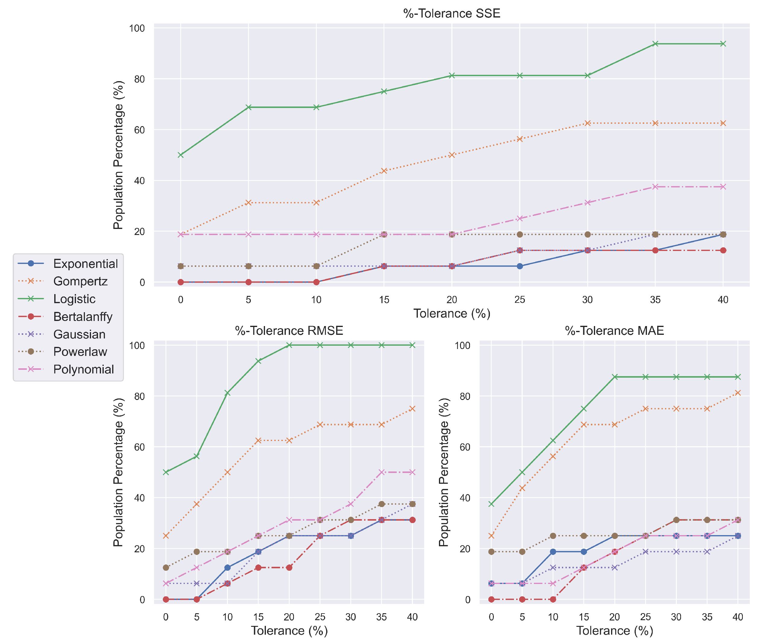
In BPPA (
Figure 2), for instance, neither the exponential, Bertalanffy, nor power law models began nor ended with good scores, showing that they cannot encompass the PA response to benzopyrene double bonds. Again, polynomials had rapid growth, but ‘logistic’ and Gompertz functions considerably outpaced the competition. The later models likewise imply analogous behavior, since both the logistic model and the Gompertz model multiplied their initial population capture. Surprisingly, the 20% divergence from the minimal scores allowed the logistic model to characterize the entire NMRI population with the BPPA mixture.
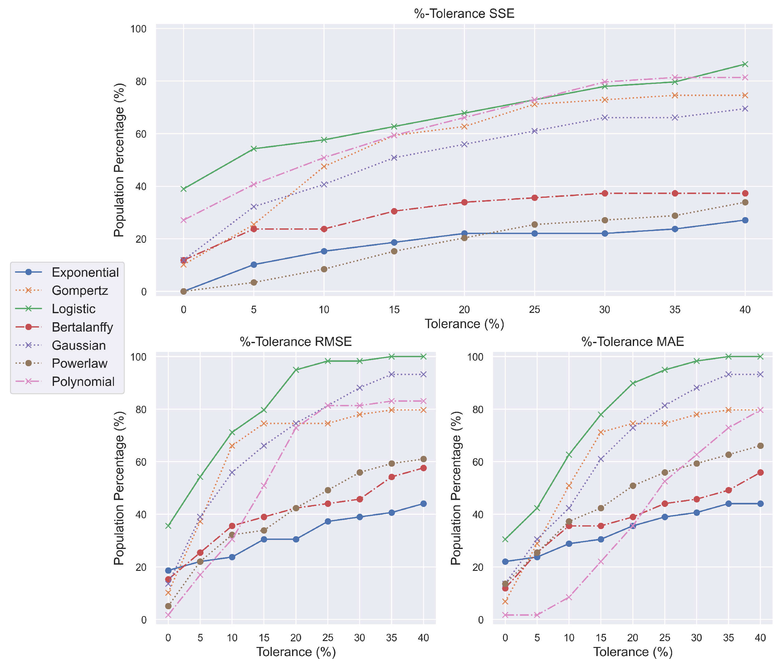
In BPTH (
Figure 3), the Gompertz growth model was initially second or third-to-last but managed to advance at least two spots by the time 20%-tolerance measurements were implemented. The power law, exponential, and Bertalanffy models displayed poor progression; however, the Gaussian model preserved an overall increase. The abrupt growth in polynomials followed by oscillations is suggested to be related to their overfitting character. Lastly, and most interestingly, the logistic function exhibits the same behavior across all measurements. It begins and ends first, maintaining a considerable margin above the other growth models. This culminates in a comprehensive description of the chemically induced oncogenesis encapsulation.
Therefore, anticarcinogenic drugs belonging to the PA and TH families can be exhaustively explained by adopting logistic models. By extension, the phenomena of oncogenesis inhibition can be described through their use, thereby simplifying the current perception of the chemical neutralization of malignant tumor development.
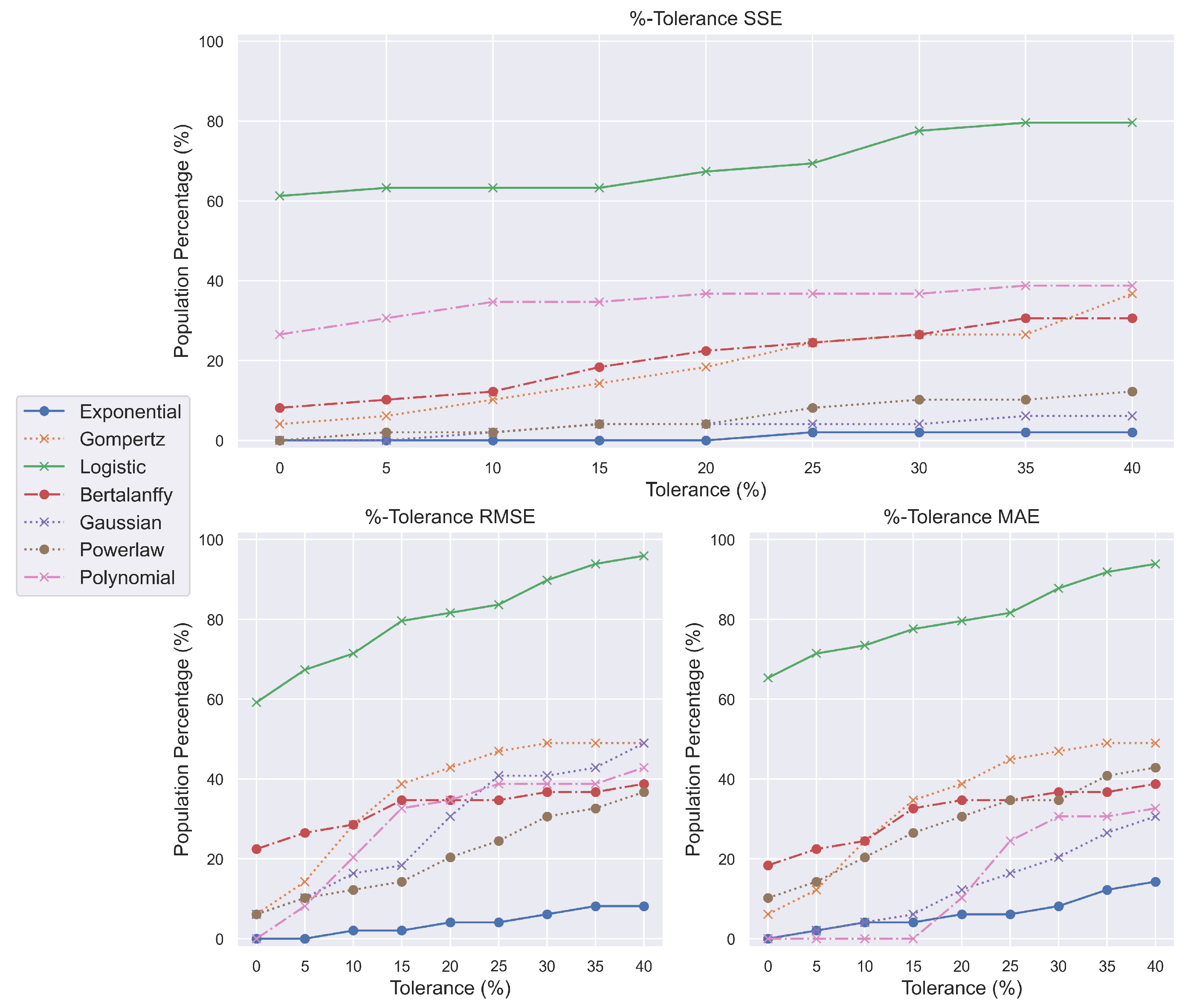
Remarkably, exponential-based models failed to account for the occurrence of chemically driven oncogenesis (
Figure 4). It is probable that the adaptability offered by sigmoid functions, such as ‘logistic’, might better suit the needs of such growth. Sigmoid functions can be segmented further into linear, exponential, and plateau phases.
The first phase describes the lag period, during which the tumor does not develop rapidly; the second phase describes the exponential growth of cancer cells; and the third phase defines the transition between the exponential and plateau phases, where the tumor has reached an advanced stage where death is inevitable. No other growth model demonstrated significant potential to comprehend chemical oncogenesis. With their greatest possible outcome, no more than fifty percent of the NMRI population can be captured.
Moving on to the statistics of the model parameters following the computational pipeline of the LMA, the vast majority of parameters have CV values larger than 30%, indicating a high degree of parameter dispersion around the mean (
Table 5). In particular, it reveals that there is no substantial central tendency, allowing for the potential that the numbers behave arbitrarily, and further supporting the notion that models with great complexity produce flexible curves. Specifically, only the Bertalanffy
parameter has an acceptable CV score, indicating the parameter’s centrality, range, and dispersion may be reliably replicated.
Despite scoring high in the statistical norm and considering the arbitrariness posed, it was further studied whether the associated parameters could be constrained in specific regions to facilitate faster reproducible results, permitting easier validation and assisting in locating the optimal values in the more variable parameters. Except for the Gaussian-based model, all models featured such a parameter. As a result, the parameter space of growth models is reduced by one dimension, simplifying the initial guessing procedure (
Table 6).
6.2. Model Predictability
Concerning model predictability, only the growth models demonstrating strong performance in the %-tolerance measurements, namely the logistic, Gaussian, and Gompertz models, were taken into account. Others are deemed incapable of adequately representing the data; hence, there is no purpose in investigating their prediction capability. From beginning to end, the employed models exhibited poor ability in predicting tumor size for the carcinogen group, as measured by a high mean difference from the ground truth. Specifically, the majority of scores were larger than 35% for the first two values (i.e., short- and medium-terms) and grew to larger than 45% for the last two (i.e., long- and extended-terms) despite the adopted model (
Table 7). This behavior results from the LMA, which received the initial data points in time as input; hence, the created curve does not yet account for the exponential growth phase, resulting in a diverging curve.
In contrast, the models produced significant results when predicting the formation of tumors in anticarcinogenic substances, particularly for starting values. In both chemical combinations, the logistic model produced the smallest difference in the short-term (0.61% and 3.59%) and maintained a close relationship with the subsequent two values (PA: 11.38% and 29.87%, TH: 13.95% and 18.82%). The Gompertz and Gaussian models displayed comparable behavior, with Gompertz exhibiting marginally superior performance in both cases. All applied functions failed to accurately predict the extended term (i.e., fourth value), indicating that we can only estimate tumor growth in the near future. Consequently, the estimates are within a respectable range (about 15%) initially, but then diverge significantly. This is primarily due to the adaptability of the models and their capacity to capture changes in cancer cell growth rates, and secondarily due to the small number of recordings made during the disease’s exponential phase. Considering that the latter four values correspond to the 20- to 40-day mice tumor inspection intervals, it is plausible to conclude that human tumor growth can be precisely predicted for two years using logistic-based models (0.61%).
Utilizing the parameters derived from the LMA convergence, a classification problem was devised not only to assess their categorization properties and, by extension, the models themselves, but also to evaluate their importance in the classification task. SVM and KNN were used as the main classifiers and were fine-tuned with cross-validation accuracy serving as the objective function.
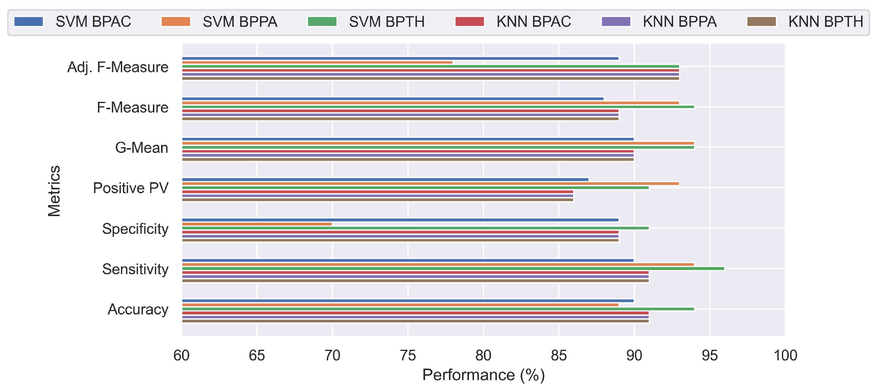
Both classifiers provide quantifiable findings and illustrate that active compounds may be distinguished, depending on model parameters exhibiting accuracy metrics above 80% across all settings (
Figure 5). Specifically, all measures have satisfactory values, with the exception of the specificity metric, whose value of 54% indicates a class imbalance. Indeed, BPPA comprises 59 data points of one class compared to 16 observations of the other class; hence, additional performance metrics were utilized, such as geometric mean, F2-measure metric, and adjusted F-measure. However, the other metrics support the excellent performance of the classifier in this particular instance. It was determined not to apply more complex classifiers, such as kernel-based algorithms, because the employed approaches were effective despite their simplicity and because advanced approaches tend to overfit in small datasets, resulting in incorrect conclusions.
The ReliefF algorithm was employed to estimate the feature contribution to the classification, and the top five features are listed in
Table 8. The contribution of the model parameters was computed based on the output of the relief algorithm, representing the significance of each feature (i.e., parameter) to the classification task. High values indicate a high importance, whereas low values indicate the opposite. By utilizing the importance value of each to the sum of all, it is possible to calculate a relative value that corresponds to the parameter contribution. It was unexpected that two parameters of the logistic model offer more than any other parameter from the set of development models, and their contribution is four times (44.47%) larger than the next closest in the BPAC classification task, which contains the most observations. It is particularly significant that the accounting model also ranks high for both its performance on %-tolerance metrics and its discriminant abilities.
Bertalanffy and Gaussian models dominate the contribution values above 5% in BPPA settings, with the former accumulating 25.49% and the latter 51.99%. However, the lack of data prevents us from providing reliable conclusions for this case. In comparison, logistic and Bertalanffy contribute 27.64% and 25.78%, respectively, to BPTH, whilst the remaining parameters have values of less than 7%, indicating that these models contribute significantly more to the relevant classification problem.
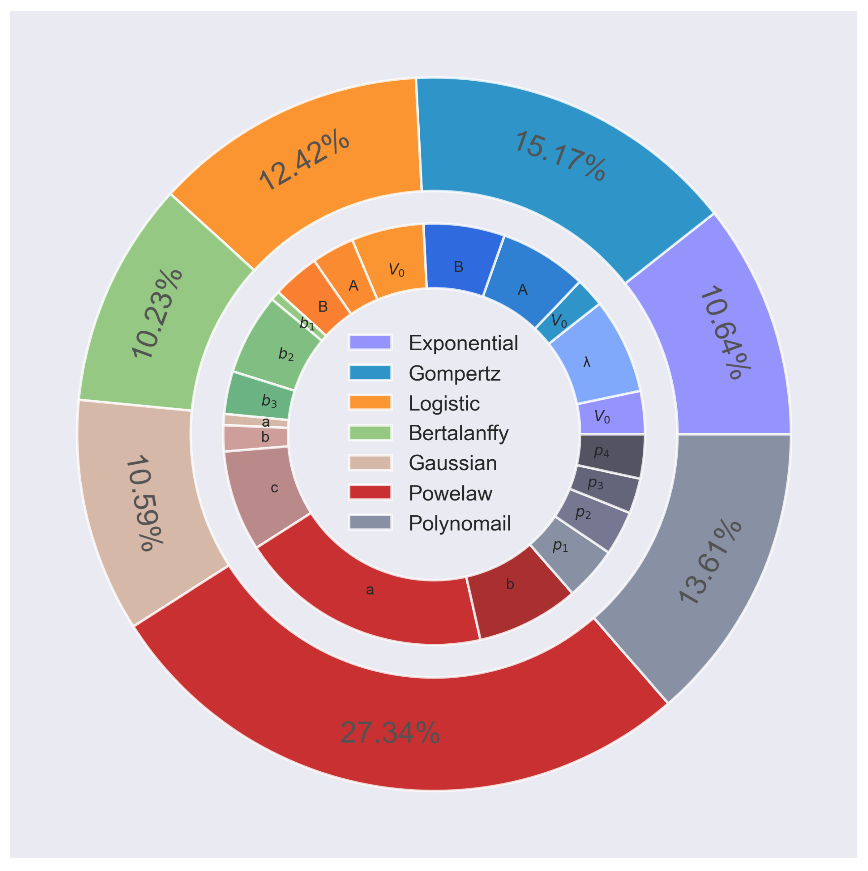
In addition, ANOVA was employed to determine the relative importance of the features. The contribution of each parameter and model to the BPAC classification task is depicted in
Figure 6. Power law generates the largest contribution (27.34%), which is to be expected for a simple model, given that the technique harnesses the variance of the experimental populations by separating it into systematic and random variables. With values ranging from 10.23% to 15.17%, the remaining growth models contribute almost the same, indicating that they are of equal importance.
6.3. Statistical Analysis
The lifespan distribution analysis, presented in
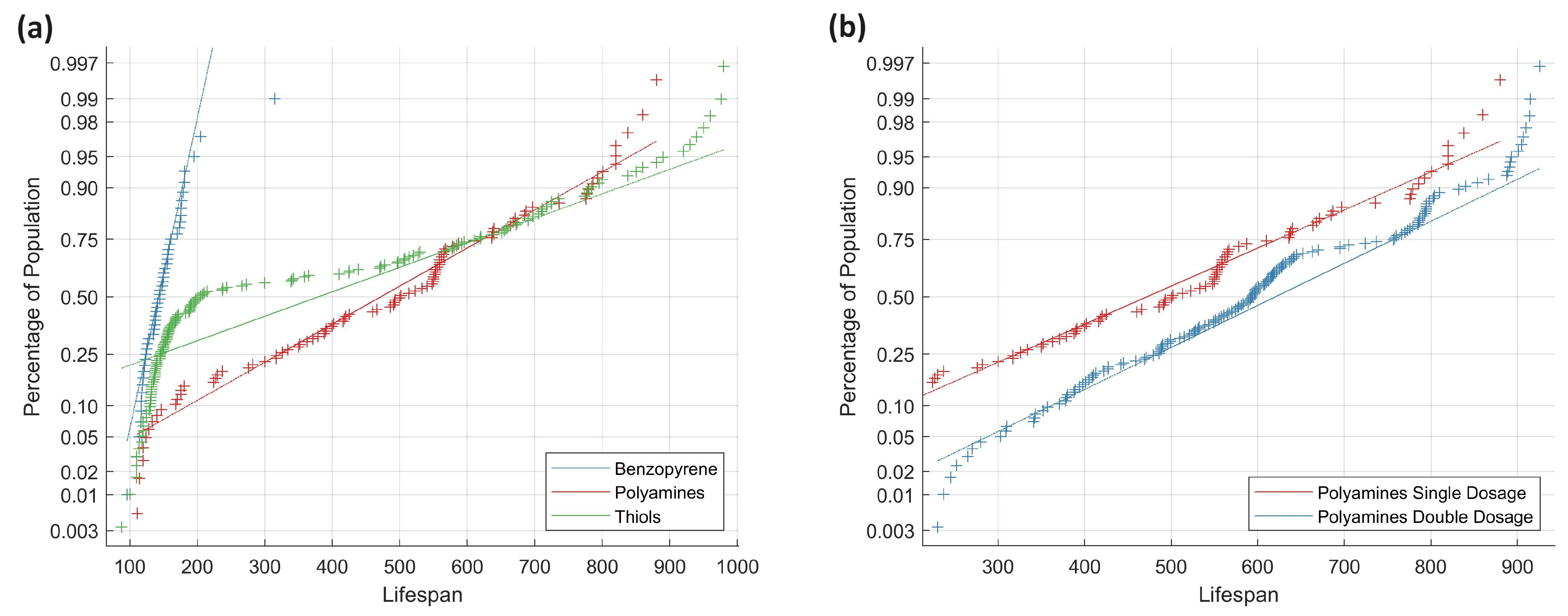
Table 9, demonstrates that single and half of the double polyamine data do not adhere to normal distributions, preventing a direct distribution comparison. This same pattern was observed in studies involving TH. To better comprehend these results, a QQ plot (
Figure 7a) was generated to graphically depict the deviation of the compound mixtures from normality and to facilitate their comparison.
The straight lines represent the normal distributions of the analyzed populations with respect to the mean and standard deviations. When lines and markers are in close proximity, this indicates normality, suggesting that the compound’s behavior can be predicted and replicated with high confidence. The behavior of the blue benzopyrene line corresponds to a 95% certainty of mortality within 200 days after administrating the carcinogenic agent. There are also outliers, with one subject dying 70 days after the injection and another surviving up to 320 days.
The most major impacts are those of PA and TH. Specifically, 45% of TH markers tend to follow the benzopyrene line with a minor delay of 10 days in the lifespan axis. Within 220 days of administering the thiol-based chemical mixture, approximately 55% of the population has perished, indicating that the behavior of TH seems to match that of benzopyrene in at least half of the population, while the other half appears to be unaffected by the disease. In contrast, PA diverges from benzopyrene from the beginning to the end, exhibiting a consistent trend toward oncogenesis inhibition. Approximately 17% of the polyamine-induced mice did not make it to 220 days, which is near the expected percentage for the species. The entire population closely matches the red line of the expected distribution of PA, demonstrating that the effect of PA may be predicted more precisely.
In examining the distribution lines, benzopyrene exhibits a steep slope (70 degrees), suggesting a high incidence, leading to species endangerment. TH and PA, with angles of 23 and 25 degrees, respectively, demonstrate effectiveness against oncogenesis, differing significantly from benzopyrene. The starting points of their lines (0.025% for PA, 0.18% for TH) contrast with the 0.003% benzopyrene, indicating a greater impact. Despite TH’s asymptotic advantage, their inconsistent behavior and higher cancer prevalence raise concerns. Both PA and TH contribute to longevity; over 20% of the population exceeds the average NMRI lifespan (700 days). Therefore, these compounds not only combat cancer uniquely but also contribute to overall health.
Figure 7b illustrates a QQ plot, comparing a single dose of PA to a twofold concentration. The parallel lines signify consistent influence but with different starting points. PA exhibits a broader impact, prompting a faster response in eradicating oncogenesis. The double dose begins at a 0.02% population impact, while the single dose starts at 0.12%, suggesting a one-sixth reduction in mortality rate. Despite minor angle differences (18 and 17 degrees), deviations from the scaled population line occur consistently in both mixtures.
This suggests two key findings: firstly, the consistent population state across initial points and degrees in both experiments; and secondly, a marginal increase in outliers, indicating extended longevity due to PA. Assuming no diminishing returns, this introduces a potential avenue for inhibiting oncogenesis and promoting longevity. The Mann–Whitney U test supports the improvement claim as the double-dose PA outperforms a single-dose (
p-value: 3.8
), suggesting increased efficacy with higher concentrations. To explain these results and better capture the data tendencies, a statistical moment analysis was conducted. Mean, standard deviation, skewness, and kurtosis, also known as the first to fourth statistical moments, were adopted to assess the mortality rate or insufficient reactions of the compound mixtures (
Table 10).
Significantly, the average longevity improves with the increasing dosage, showing that the chemicals are more effective at higher concentrations. The standard deviation represents the degree of value dispersion around the mean, which initially varies substantially and diminishes as dosage increases. The skewness of symmetrical distributions, such as mortality distributions, should be near zero. Benzopyrene does not adhere to this criteria because of its asymmetry. PAs have a tendency to approach zero on both sides. Regarding the mortality rate, it is evident that a single dose of PA reduced the mortality rate by at least 80%; however, a double dose of PA outperformed the other mixes by producing an astounding performance in which just 1.34% of the population perished.
7. Discussion
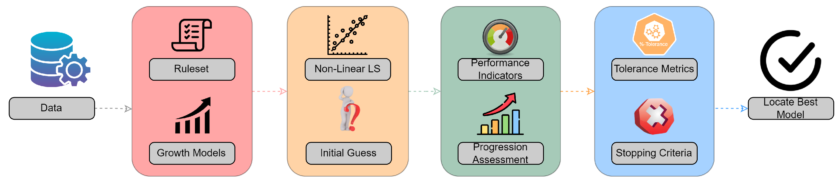
The analysis presented herein aims to explain the process of chemical oncogenesis and inhibition using mathematical functions that, when applied to data, become models. Surgical administration of benzopyrene, a chemical carcinogen capable of causing tumors with certainty, was employed to trigger chemical oncogenesis. In an effort to neutralize the carcinogenic agent, PA and TH were supplied in addition to benzopyrene to strengthen the immune system or fight cancer, respectively. These compounds, which are abundant in nature, can modify the structure of an oncogenic agent to resemble that of a less cancerous agent. In 1978, the Laboratory of Physiology at the University of Ioannina in Greece began conducting research with more than 400 NMRI subjects. These experiments led to the establishment of a dataset based on tuples consisting of tumor sizes and examination dates. The examinations were performed at specific intervals using ultrasonic tomography. Utilizing this dataset, an attempt was made to formalize an explanation workflow for the phenomena of oncogenesis and inhibition was developed (
Figure 1).
However, this approach might be used in other applications that utilize past knowledge to deliver valuable insights. Initially, a rule set was designed to outline the conditions that growth models must satisfy. In this instance, three criteria were devised to evaluate the produced models and identify the one with the most descriptive power. The primary criteria synthesized involved adequately approximating various data series, reflecting comparable behavior, and avoiding fluctuations between optimal and poor outcomes. After establishing these rules, a multitude of mathematical functions were utilized to evaluate how these phenomena may be interpreted and anticipated. Sigmoid functions, which mimic homeostasis because they include linear, exponential, and plateau phases, were also used. A curve-fitting pipeline was orchestrated based on the collected data, with a focus on addressing the initial guess problem.
After LMA convergence, SSE, RMSE, and MAE served as primary performance indicators. To provide insight into model performance on the remaining data series, tolerance metrics were introduced. These metrics allowed for incremental encapsulation of model progression without sacrificing descriptiveness. In most cases, the logistic model outperformed competitors, demonstrating consistent behavior and capturing the entire population before 30%-tolerance metrics (
Table 4,
Figure 2,
Figure 3 and
Figure 4). Exploring oscillations, surprises, and abrupt growth, logistic models proved effective in explaining anticarcinogenic drugs and carcinogenic chemicals, simplifying the understanding of tumor inhibition and oncogenesis. Growth model parameters were evaluated for central tendency and parameter intervals with less variation, facilitating future reproduction and validation (
Table 5 and
Table 6). Logistic models excelled in forecasting tumor growth, particularly in the case of PA (
Table 7). Classification problems with growth parameters as features demonstrated SVM’s superiority in distinguishing between compound combinations (
Figure 5). Logistic function parameters exhibited the highest contributions in ReliefF and ANOVA in specific settings (
Table 8,
Figure 6). Normality tests of NMRI mortality, regardless of cancer presence, yielded inconclusive results. The factors contributing to this nature may include a relatively modest sample size, with the potential deviation of the underlying data distribution from normality, and the inherent complexity of the phenomenon under investigation, rendering it challenging to derive definitive conclusions (
Table 9). For this reason, QQ plots were employed, which illustrated distinct compound combination responses and suggested the potential for a triple dosage. PA, as an alternative cancer combatant, exhibited a longer average lifespan, lower mortality rate, and stability that was positively influenced by concentration increases (
Figure 7a,b).
The transition from bench-side to bedside research is illustrated by the pragmatic implications of scientific findings in oncology. Mathematical models, integrating data from surgical experiments and ultrasonic examinations, establish an algorithmic framework to understand and predict tumor behavior over time. This paradigm shift facilitates the translation of scientific insights into actionable clinical strategies, which was revealed by the experimental inclusion of PA and TH as chemopreventive measures. The developed mathematical models not only elucidate oncogenic mechanisms but also provide clinicians with practical tools for anticipating and managing tumor growth, enhancing the efficacy of cancer treatments. These models, based on tumor size and examination dates, coupled with ultrasonic tomography, are invaluable for tailoring treatment strategies, forecasting growth patterns, and optimizing therapeutic interventions. The consistent performance of the logistic model, especially in forecasting tumor growth in response to PA, signifies its transformative potential, enabling personalized treatment plans based on individual tumor dynamics and addressing complex clinical scenarios with a classification framework for compound combinations.
In contrast to previous chemoprevention-related work that either prioritized the theoretical background of compound discovery without numerical evidence or provided substantial evidence without the physiological basis for delaying or preventing cancer development, this study proposes an algorithmic pipeline of mechanisms. This pipeline uses a ruleset as a foundation to investigate the best descriptive power among a plethora of mathematical functions capable of explaining the phenomena of oncogenesis and chemical inhibition, while supporting it with chemical reaction theory. By pursuing this path, the potential to explain chemoprevention and other significant occurrences increases substantially, necessitating the selection of the most appropriate descriptive model among others. Mechanisms such as those presented can circumvent this barrier, allowing the scientific community to establish a baseline and construct more complex and seasoned schemes on top of it.
The resulting analysis is not without shortcomings and limitations. The inclusion of a modest number of ultrasonic examinations in the data collection may impact the reliability of chemoprevention outcomes. Sparse examinations, separated by over 40 days, limit insight into the precise onset of oncogenesis and its progression rate. Ethical concerns surrounding frequent exams, linked to potential cancer development from computed tomography scans, further constrain data acquisition. Additionally, the study raises concerns about heightened side effects and increased toxicity due to the novel approach of escalating compound concentrations for cancer chemical inhibition. While no subjects in this study experienced such issues, it is noteworthy that previous research reported two NMRI mice deaths attributed to probable putrescine toxicity [
49]. This underscores the need for vigilant consideration of potential risks, ensuring safety and ethical integrity in experimental protocols.
In conclusion, this comprehensive discussion highlights the noteworthy contributions and limitations of the study in advancing our understanding of chemopreventive strategies and personalized cancer therapy. The developed mathematical models, incorporating PA and TH, bridge the gap between experimental and clinical realms, opening up promising avenues for cancer prevention. The logistic model’s consistent performance suggests its potential application in tailoring personalized treatment plans. Despite the challenges posed, including a modest sample size, sparse examinations, inconclusive statistical tests, and the potential toxicity produced by the chemicals, the study’s classification framework and algorithmic pipeline provide a versatile foundation for addressing complex clinical scenarios. The contextual specificity of the research design and subject characteristics must be acknowledged, as generalization challenges may restrict findings to specific populations or experimental settings. Therefore, this research not only propels the field forward but also underscores the complexities and variations inherent in studying cancer dynamics and therapeutic interventions. As we navigate these difficulties, the study lays a foundation for future investigations, emphasizing the importance of robust methodologies, ethical considerations, and a continual commitment to refining our understanding of cancer biology and treatment.


 and
and 


