
Ground Truth in Classification Accuracy Assessment: Myth and Reality


School of Geography, University of Nottingham, Nottingham NG7 2RD, UK
Geomatics 2024, 4(1), 81-90; https://doi.org/10.3390/geomatics4010005
Submission received: 20 December 2023
/
Revised: 12 February 2024
/
Accepted: 13 February 2024
/
Published: 16 February 2024
Abstract
:The ground reference dataset used in the assessment of classification accuracy is typically assumed implicitly to be perfect (i.e., 100% correct and representing ground truth). Rarely is this assumption valid, and errors in the ground dataset can cause the apparent accuracy of a classification to differ greatly from reality. The effect of variations in the quality in the ground dataset and of class abundance on accuracy assessment is explored. Using simulations of realistic scenarios encountered in remote sensing, it is shown that substantial bias can be introduced into a study through the use of an imperfect ground dataset. Specifically, estimates of accuracy on a per-class and overall basis, as well as of a derived variable, class areal extent, can be biased as a result of ground data error. The specific impacts of ground data error vary with the magnitude and nature of the errors, as well as the relative abundance of the classes. The community is urged to be wary of direct interpretation of accuracy assessments and to seek to address the problems that arise from the use of imperfect ground data.
1. Introduction
The expression ground truth has been used widely in geomatics. It is a term that implies a perfect or completely truthful representation of the relevant aspect of the world under study (e.g., land cover class, building height, etc.). Rarely will any dataset be perfect, and hence, some degree of error is likely to exist. Because of this situation, many researchers avoid the expression ground truth and use terms such as ground or reference data instead. While the latter terms show an awareness of a major limitation with ground datasets, they do not actually address the impacts that arise as a function of using an imperfect ground dataset. Here, the focus is on some issues that arise in classification studies, such as those used to generate thematic information from remotely sensed data.
The ground data used in an image classification have a fundamental role in the analysis and interpretation of the results obtained. In popular supervised image classifications, ground data are used to train and assess the accuracy of the classification analysis. A variety of myths about classification analyses exist and are embedded in the community’s standard practices. Some myths relate to methods used and their assumptions about the data. For example, fundamental assumptions about the data may be untenable (e.g., pure pixels, exhaustively defined set of classes, etc.), and the metrics used in accuracy assessment may be inappropriate [1] or may not possess attributes often claimed [2]. Here, some interlinked issues on the nature of the classes and ground data used in accuracy assessment, notably related to class abundance and data quality, are flagged to help encourage the research community to more fully address ground data imperfections in research. Writing this opinion piece occurred when finalising an article [2] on the impacts of using an imperfect reference standard on the interpretation of a range of classification accuracy metrics. The latter provides a foundation here to flag some key issues associated with the typical absence of ground truth on classification accuracy assessment in geomatics.
Fundamentally, an accuracy assessment involves the comparison of the class labels predicted by a classifier against those observed in reality. The latter is the ground truth, which provides a perfect characterisation of reality and is, therefore, a true gold standard reference. A basic and widely used metric of classification accuracy is simply the proportion of cases that the classifier labelled correctly, often expressed as a percentage and referred to as overall accuracy. Although this is a legitimate approach to use in an accuracy assessment and does convey some useful information, it is not well-suited for use as a metric of overall accuracy [3,4,5]. Two well-known but often ignored concerns with the metric are relevant here. First, the relative abundance of the classes can impact the analysis. If the classes are imbalanced, a poor classifier that simply tends to allocate labels to a relatively abundant class could appear more accurate and useful than it is [6]. Second, the ground dataset is rarely perfect and hence contains error. In essence, ground truth is typically a mythical entity; it rarely exists, and an imperfect characterisation of reality is normally used as a reference in accuracy assessment. The imperfections in the ground data can cause substantial biases in an accuracy assessment and complicate interpretation because the use of a gold standard reference is implicitly assumed in the analysis [2]. The failure to satisfy this assumed condition leads to misestimation of accuracy, misinterpretation of results, and potentially incorrect decision-making.
The problems associated with relative class abundance and ground data quality on an accuracy assessment are well-known and can be illustrated with a basic binary classification. This type of classification is widely encountered in geomatics, for example, in studies of change such as deforestation or when attention is focussed on a specific class such as an invasive species. Here, the generic class names of positive and negative are used for convenience. The relative abundance of the classes (often referred to as prevalence) can be quantified as the ratio of the true number of positive cases to the total sample size. When this ratio is 0.5, the two classes are of equal size. The classes are imbalanced as the ratio deviates from 0.5. For example, the smaller the value, the rarer the positive class is in the dataset. The accuracy assessment itself is typically based on a confusion matrix formed by the cross-tabulation of the classifier’s predicted labels against the corresponding ground data labels for a sample of cases. Good practice advice for undertaking the accuracy assessment exists [7] and underpins major applications such as in support of environmental policy [8]. While these good practices recognise that problems exist with ground data, they do not fully address them. For example, the good practice advice encourages the use of a ground reference dataset that is more accurate than the classification being evaluated [7], but this does not act to reduce or remove the biases caused by the data imperfections that are present. Here, the aim is to give a guide to the magnitude of the problems of using an imperfect ground dataset in classification accuracy assessment to raise awareness of key issues and encourage activity to address them.
2. How Accurate Are Ground Data?
The literature provides a guide to the accuracy of ground datasets used in geomatics. For example, expert image interpreters are often used to generate ground data. Typically, a small group of experts is provided with fine spatial resolution imagery for a set of locations and other relevant materials such as a classification key that may aid in labelling. The degree of agreement between the experts in their labelling of the same set of images provides a guide to the accuracy of the labels. Agreement is only an imperfect indicator of the accuracy of labelling because it is, for example, possible for experts to incorrectly agree on their labelling, and in such circumstances, accuracy is less than indicated by agreement.
In a study focused on mapping ponded water and slush on ice shelves, [9] observed large levels of inter-expert disagreement. Specifically, [9] show the average level of agreement for ponded water and slush to be 78% and 71%, respectively. In addition, the level of agreement observed was found to vary geographically between test sites [9]. Similarly, [10] assessed the level of inter-expert agreement for class labelling in a highly fragmented landscape in Amazonia. Specifically, [10] report an average level of inter-expert agreement of 86%. In addition, they note substantial differences in inter-expert agreement between land cover classes. For example, inter-expert agreement for second growth forests was just 48.8%, but 92.1% for primary forest [10]. Other terrestrial features interpreted from remotely sensed imagery may be imperfectly characterized. For example, in mapping geomorphological features such as eskers from Landsat imagery, [11] noted that 75% of esker ridges were correctly identified, while the remaining 25% were missed mainly because of their small size relative to the spatial resolution of the imagery used. Critically, studies such as those by [9,10,11] highlight substantial disagreement and error in the labelling of features from imagery by experts. Crudely, this literature suggests that the overall magnitude of the error in a dataset could often be up to 30%, but with variation between classes and in space.
Other studies that have explicitly addressed the quality of ground datasets confirm that large errors may exist. For example, [12] refers to a ground dataset with an overall accuracy of 82.4%. Such studies recognise the existence of relatively large error levels but also satisfaction with the datasets. For example, [12] highlight that the dataset with an overall accuracy of 82.4% “can be considered as a satisfying reference” ([12], p. 3189). Thus, our community appears to be aware of the existence of ground data error and comfortable with what appear to be large error rates.
The concern with ground data quality is not limited to simply the magnitude of mis-labelling. A further issue of concern is the nature of the errors and, in particular, the degree of independence of errors in the image classification to be assessed and the ground dataset. If the errors in the classification and ground data tend to occur with the same cases, the errors are conditionally dependent or correlated. This type of error may be expected to arise when the process of labelling in the image classification and ground data is the same or similar. This situation might be expected to occur in contemporary remote sensing research as the ground data often arise from analysis of imagery with a finer spatial resolution than that used to generate the classified image. Independent errors might arise when the process of labelling in the two datasets is different. For example, if the ground data labelling was based on field observation and hence used a set of attributes different from those used in classifying the imagery. The distinction between independent and correlated errors is important as they have a major influence on the direction of mis-estimation [2]. The relative magnitude of omission and commission errors as well as differences in class size can also impact on the assessment of classification accuracy.
3. Materials and Methods
For illustrative purposes, the estimation of classification accuracy under a range of circumstances can be simulated [2]. Here, a binary classification that meets a common albeit questionable accuracy target used in geomatics research will be assessed using ground datasets of variable quality and over the range of possible class imbalances. Throughout, the classification being evaluated was 85% correct with each class classified to the same accuracy (i.e., producer’s accuracy of each class was 85%).
Two sets of analyses were undertaken. First, the accuracy of a classification was assessed using a perfect ground reference dataset (i.e., 100% correct) and also with very high-quality ground datasets for three scenarios (Table 1). The values used in the simulations are relatively arbitrary, but to keep relevance to real-world applications, they were based on recently published research. Considerable attention has recently focused on mapping terrestrial water bodies, and very high accuracies calculated on a per-class and overall basis have been reported (e.g., [13,14,15]). Nonetheless, small errors may occur in the ground data. In a discussion on the quality of the ground data, [13] report commission errors of a little less than 1% and omission errors a little less than 5%. One specific case presented by [13] was taken to form scenario I (Table 1). Scenario I is based explicitly on actual estimates of ground data quality. Two other scenarios, scenarios II and III, were explored. These were based on recent classification studies by [15], and while not explicitly based on ground data quality, they involve highly accurate classifications and are compatible with values indicated by [13]. For example, the levels of error in the two ground datasets in scenarios II and III were small, with omission errors over the two classes of 0.4%, 0.5%, 1.5%, and 5.2%. Scenarios II and III do have important differences, notably in the relative accuracy of the positive (water) and negative (no-water) classes.
For all three scenarios, the assessments of classification accuracy were made relative to two simulated ground datasets, one containing correlated errors and the other containing independent errors. These simulations provide examples to illustrate key issues based on realistic conditions for real-world applications. The simulations are focused on mapping to a level often used as a target (overall accuracy of 85%) and basing the accuracy assessment on very high-quality ground datasets.
To further illustrate issues connected to the magnitude of ground data error and the impact of variations in class abundance, a further set of analyses were undertaken. Again, the classifier under evaluation was 85% correct. This classification was then assessed relative to five ground datasets. First, an error-free, true gold-standard dataset was used to illustrate the result obtained when the assumption of ground truth was valid. The assessment was then repeated using imperfect ground datasets. The latter had two levels of error. One ground dataset was marginally more accurate (overall accuracy = 86%, classes have equal producer’s accuracy), and the other was substantially more accurate (overall accuracy = 95%, classes have equal producer’s accuracy) than the classification under-assessment. These latter assessments were undertaken twice, once with the errors in the ground data conditionally independent of those in the classification and again with the errors correlated with those in the classification. As noted above, both situations could be expected to occur in remote sensing applications. For example, correlated error can be expected if the labelling is based on the same phenomenon or process. Alternatively, independent errors might emerge if the labelling arises in a different way, perhaps from authoritative field work or, increasingly, provided by citizens [16]. Such labelling may be based on very different attributes than those used in an image classification but still may be imperfect and represent a challenge for the successful use of such data [17]. Details on the calculations that underpin the simulations are given in [2] and are based on the approaches of [18] and [19] for independent and correlated errors, respectively.
Many metrics of classification accuracy may be calculated for a binary classification [20]. These metrics make variable use of the content of the four elements of a binary confusion matrix: true positives (TPs), true negatives (TNs), false positives (FPs) and false negatives (FNs). Here, the focus is on just four metrics that are widely used in geomatics. For per-class accuracy, the metrics were the producer’s and user’s accuracy for the positive class, sometimes referred to as recall and precision, respectively. These metrics can be calculated from:
and
The other two metrics of accuracy assessed are often used to provide a guide to the overall accuracy of a classification. The metrics were F1 and the Matthews correlation coefficient (MCC). F1 has been widely promoted, especially in cases of concerns about class balance [21], and the MCC has been promoted as a truthful metric for all classification analyses in all subject areas [22]. These metrics can be calculated from:
and
The values of each of the four accuracy metrics are positively related to classification quality and lie on a 0–1 scale. Sometimes, the value calculated is multiplied by 100 and expressed as a percentage. The issues reported in this article are explored further with a wider set of accuracy metrics in [2].
A large number of other metrics are available for use in accuracy assessments (e.g., [1,20,23,24]). Like F1, some are essentially combinations of basic metrics. For example, the receiver operator characteristic curve (ROC), and especially the area under this curve, has been widely used in accuracy assessments. The ROC is based on the producer’s accuracy, calculated for both the positive and negative classes. Clearly, if the calculation of the producer’s accuracy for a class is impacted by issues such as class balance and ground data error, then metrics based upon it would also be impacted, the exact nature of the impact depending on the specific circumstances. Additional concerns have also been noted when using the area under the ROC for the assessment of binary classifications [25,26]. Critically, an accuracy assessment may be expected to be erroneous and potentially misleading whatever metric is used if the ground data are imperfect.
4. Results and Discussion
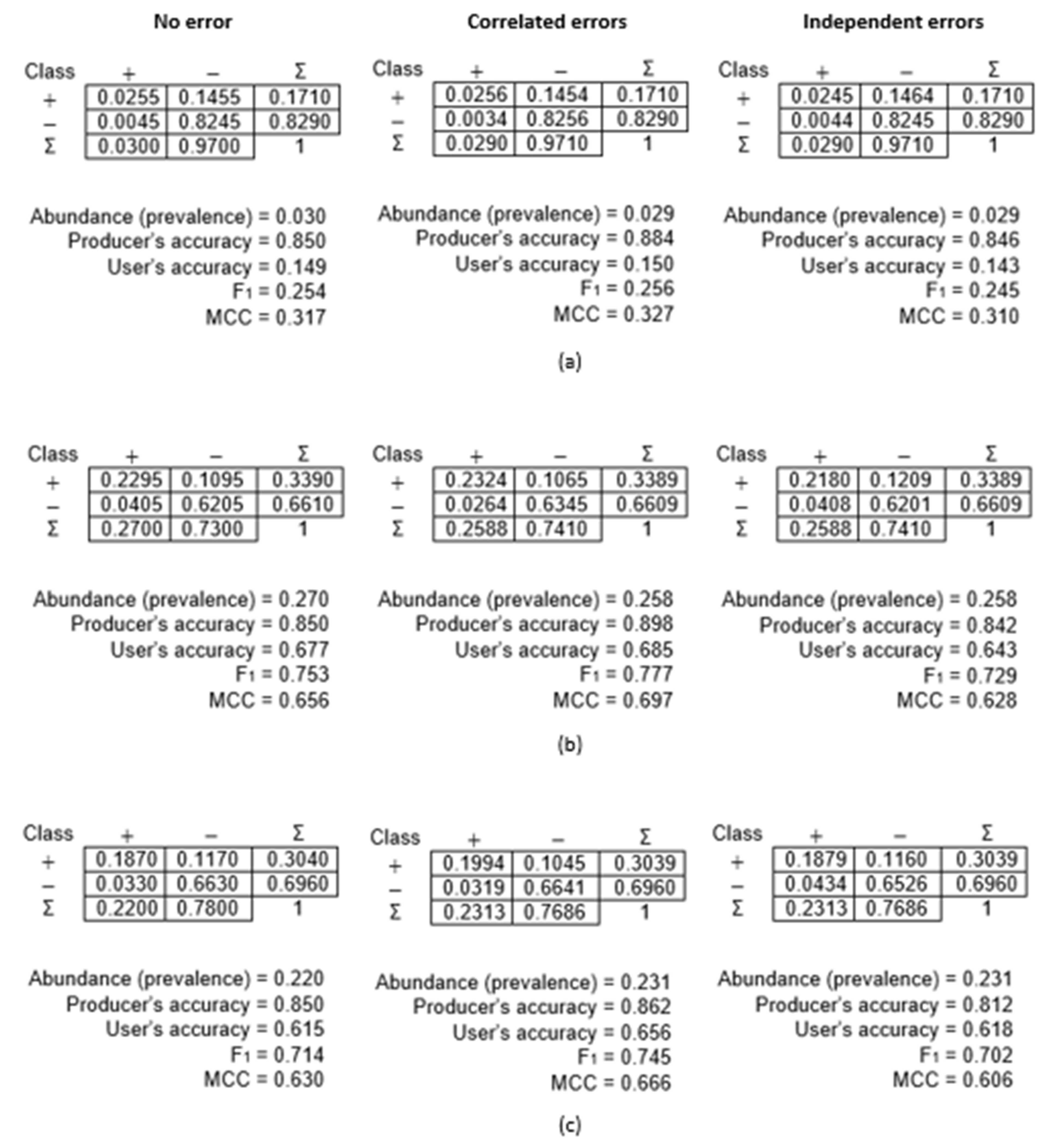
The confusion matrices and associated apparent accuracy values arising from the simulations based on mapping water and using very high-quality ground datasets are shown in Figure 1. The key feature to note is that the confusion matrices and the measures calculated from them differ depending on which ground dataset was used. Note, for example, that with the ground dataset containing correlated errors, all four accuracy metrics were overestimated for scenario I (Figure 1a). What constitutes a significant and meaningful mis-estimation will vary from study to study, but critically, relatively large misestimation may arise even when a very high-quality ground dataset is used. This is particularly evident in scenario I for the producer’s accuracy, which was estimated at nearly 89% instead of 85% (Figure 1a). Conversely, with the use of the ground dataset containing independent errors, all four accuracy metrics were underestimated (Figure 1a).
Misestimation was also evident in the results for scenarios II and III (Figure 1b,c). Key trends remain, such as all four accuracy metrics being overestimated when the reference dataset contains correlated errors. But there are notable differences between scenarios II and III illustrated in Figure 1. For example, with scenario II (Figure 1b), it is evident that abundance is slightly underestimated while it is overestimated in scenario III (Figure 1c). Additionally, the user’s accuracy is over-estimated in scenario III with the use of each imperfect ground dataset, unlike the other two scenarios in which overestimation is associated with the use of the ground dataset containing correlated errors (Figure 1). Differences between scenarios II and III in Figure 1b,c are, in part, linked to the small difference in abundance of water but especially to the dissimilar nature of the errors in the ground datasets. Note in scenario II, the producer’s accuracy of the negative class was larger than that for the positive class, while the opposite situation occurred in scenario III (Table 1). The relative magnitudes of the errors of omission and commission combined with relative class abundances can have a marked impact on the analysis. Critically, the size and nature of errors in the ground dataset, even if small, can therefore have a marked impact on an accuracy assessment even when the magnitude of error in the ground dataset is low.
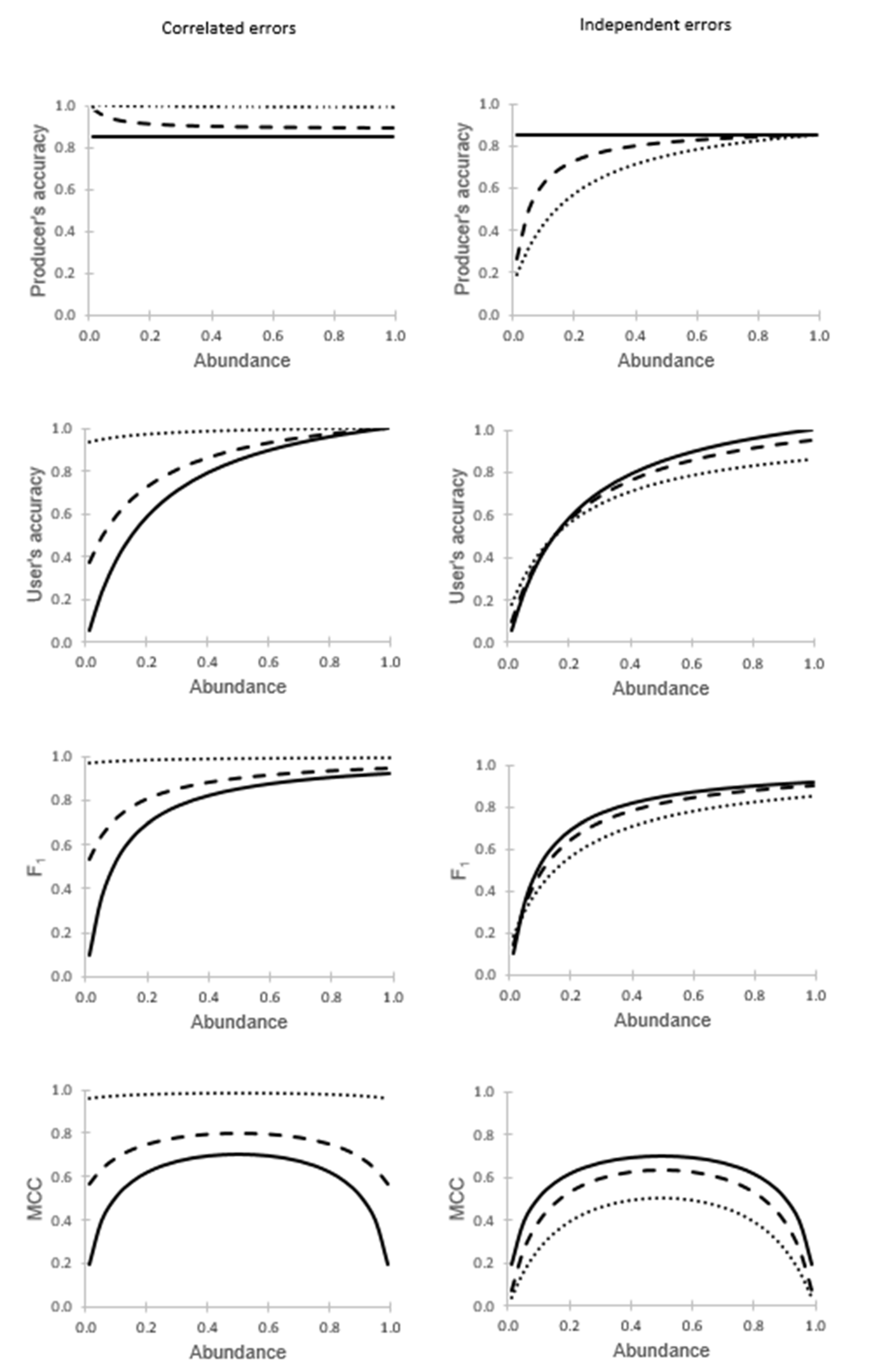
The second set of analyses focused on variations in class abundance and ground data quality. Variations in both class abundance and ground data quality had substantial effects on all four accuracy metrics assessed (Figure 2). In every scenario assessed, in which the producer’s accuracy for the two classes in the ground dataset were of equal magnitude, it was evident that classification accuracy was misestimated, deviating from the true accuracy estimated with a gold standard reference (shown as the solid black line). The magnitude of misestimation varied with the relative abundance of the classes and was also positively related to the degree of error in the ground dataset. One feature to note is that substantial misestimation could be observed when the ground dataset was very accurate (e.g., the producer’s accuracy at very low values of abundance drops from 85% to 15% when the errors were independent).
The direction of the bias in the apparent classification accuracy observed was dependent on the nature of the errors in the ground dataset. With correlated errors, it was evident that classification accuracy, assessed by all four metrics, was overestimated. Conversely, the accuracy metrics tended to be underestimated if the errors were independent; two small exceptions to the general trend are observed for user’s accuracy and F1 at low values of abundance (Figure 2).
It was also evident that for all of the metrics, the apparent value of accuracy varied with the relative abundance of the classes. Note that this includes the producer’s accuracy, a metric often claimed to be independent of abundance (prevalence). The theoretical independence of abundance that exists for this metric is lost with the use of an imperfect ground dataset.
Lastly, derived products may also be misestimated. For example, there is often interest in the areal extent of the classes, which is indicated by the relative abundance. As noted in earlier analyses (Figure 1), when an imperfect ground dataset is used, not only is accuracy misestimated but so too are estimates of class extent. As a guide, for the specific scenarios illustrated, the areal extent of the positive class tended to be overestimated when it is rare in the classification set and overestimated if it is more abundant than the negative class. The magnitude of misestimation is greatest at extreme values of class abundance. To illustrate the magnitude of the issue, when the real abundance was 0.01 (i.e., 1%) and the ground dataset that was 86% accurate was used, the apparent abundance is nearly 15 times larger than the true value at 0.147. The exact nature of the misestimation will depend on the specific circumstances (e.g., inter-class differences in error levels, Figure 1).
The misestimation of accuracy and class abundance due to the use of an imperfect reference is well-known yet rarely is anything done about it [2,4]. There are, however, a variety of actions that can be taken to help address the problems associated with the use of an imperfect ground dataset. First, the problems need to be recognised and apparent values of accuracy and/or class area treated with caution. Researchers should avoid naïve use of apparent values of classification accuracy and class areal extent, recognising the need to be wary of interpreting them directly. Rather, the impacts of the imperfect reference should be accounted for. A range of approaches to address the problem of an imperfect ground dataset exist [27]. Researchers could, for example, estimate the quality of the ground data and use this to calculate true values. The correction of apparent values to true values is relatively straightforward if the errors are known and independent [18] but can still be undertaken when the errors are initially unknown and correlated [19]. An alternative approach is to essentially construct a reference standard by combining results from a series of imperfect classifications applied to a dataset [27]. One such approach is based on latent class analysis. This latter analysis can be used to estimate classification accuracy from the pattern of results obtained by applying multiple classifiers to the dataset. This is simple in remote sensing as a range of different methods of classification are available for application to a dataset (e.g., [28,29]). This approach can also be used with both independent and correlated errors. Latent class analysis has been used to estimate both image classification accuracy [30] as well as the accuracy of data provided by citizens, which could be used as ground data [31]. Other studies have further illustrated the potential of model-based methods and inference when ground data are limited or unavailable [32,33].
5. Conclusions
Ground truth is implicitly assumed to be used in a classification accuracy assessment, yet it rarely exists. Error in the ground data will introduce potentially large biases, and the resulting apparent values of classification accuracy can differ greatly from reality. This situation can lead to misinterpretation, and ultimately, poor decision-making. The magnitude of the problems associated with error in the ground dataset will vary with the amount and nature of the errors.
The concerns noted here about ground data quality are well-known yet rarely addressed. Action to address the impacts of using an imperfect reference, however, should be undertaken as the impacts can be large and are likely to be commonplace. Indeed, if gold standard reference data are rare, then it follows that incorrect accuracy assessments are superabundant. Being provocative, the apparent accuracy of classifications and of derived products such as estimates of class areal extent reported in the geomatics literature are open to substantial error and misinterpretation. The reality is that most (virtually all?) accuracy assessments are biased because of the use of an imperfect reference.
The research community needs to go beyond recognizing that problems with ground data exist to actually addressing them. Additionally, while the focus in this opinion piece was on accuracy assessment, it should be noted that error in the ground data used to train a classification also requires attention as it can degrade the analysis [34,35,36,37]. Variations in class abundance also impact the training of image classifications [38]. Critically, ground truth is often a myth, and the reality is that imperfect ground data are typically used in classification analyses, which can have potentially large negative impacts. Addressing the issue of imperfect ground data will help realise the full potential of geomatics and the applications that depend on it.
Funding
This research received no external funding.
Acknowledgments
I am grateful to the four referees and editor for their comments on the original manuscript.
Conflicts of Interest
The author declares no conflicts of interest.
References
- Pontius, G.R., Jr. Metrics That Make a Difference; Springer: Cham, Switzerland, 2022. [Google Scholar]
- Foody, G.M. Challenges in the real world use of classification accuracy metrics: From recall and precision to the Matthews correlation coefficient. PLoS ONE 2023, 18, e0291908. [Google Scholar] [CrossRef] [PubMed]
- Shao, G.; Tang, L.; Liao, J. Overselling overall map accuracy misinforms about research reliability. Landsc. Ecol. 2019, 34, 2487–2492. [Google Scholar] [CrossRef]
- Halladin-Dąbrowska, A.; Kania, A.; Kopeć, D. The t-SNE algorithm as a tool to improve the quality of reference data used in accurate mapping of heterogeneous non-forest vegetation. Remote Sens. 2019, 12, 39. [Google Scholar] [CrossRef]
- Stehman, S.V.; Wickham, J. A guide for evaluating and reporting map data quality: Affirming Shao et al. “Overselling overall map accuracy misinforms about research reliability”. Landsc. Ecol. 2020, 35, 1263–1267. [Google Scholar] [CrossRef]
- Türk, G. GT index: A measure of the success of prediction. Remote Sens. Environ. 1979, 8, 65–75. [Google Scholar] [CrossRef]
- Olofsson, P.; Foody, G.M.; Herold, M.; Stehman, S.V.; Woodcock, C.E.; Wulder, M.A. Good practices for estimating area and assessing accuracy of land change. Remote Sens. Environ. 2014, 148, 42–57. [Google Scholar] [CrossRef]
- Penman, J.; Green, C.; Olofsson, P.; Raison, J.; Woodcock, C.; Balzter, H.; Baltuck, M.; Foody, G.M. Integration of Remote-Sensing and Ground-Based Observations for Estimation of Emissions and Removals of Greenhouse Gases in Forests: Methods and Guidance from the Global Forest Observations Initiative, 2nd ed.; Food and Agriculture Organization: Rome, Italy, 2016. [Google Scholar]
- Dell, R.L.; Banwell, A.F.; Willis, I.C.; Arnold, N.S.; Halberstadt, A.R.; Chudley, T.R.; Pritchard, H.D. Supervised classification of slush and ponded water on Antarctic ice shelves using Landsat 8 imagery. J. Glaciol. 2022, 68, 401–414. [Google Scholar] [CrossRef]
- Powell, R.L.; Matzke, N.; de Souza, C., Jr.; Clark, M.; Numata, I.; Hess, L.L.; Roberts, D.A. Sources of error in accuracy assessment of thematic land-cover maps in the Brazilian Amazon. Remote Sens. Environ. 2004, 90, 221–234. [Google Scholar] [CrossRef]
- Storrar, R.D.; Stokes, C.R.; Evans, D.J. Morphometry and pattern of a large sample (>20,000) of Canadian eskers and implications for subglacial drainage beneath ice sheets. Quat. Sci. Rev. 2014, 105, 1–25. [Google Scholar] [CrossRef]
- Robinson, C.; Malkin, K.; Jojic, N.; Chen, H.; Qin, R.; Xiao, C.; Schmitt, M.; Ghamisi, P.; Hänsch, R.; Yokoya, N. Global land-cover mapping with weak supervision: Outcome of the 2020 IEEE GRSS data fusion contest. IEEE J. Sel. Top. Appl. Earth Obs. Remote Sens. 2021, 14, 3185–3199. [Google Scholar] [CrossRef]
- Pekel, J.F.; Cottam, A.; Gorelick, N.; Belward, A.S. High-resolution mapping of global surface water and its long-term changes. Nature 2016, 540, 418–422. [Google Scholar] [CrossRef]
- Pickens, A.H.; Hansen, M.C.; Hancher, M.; Stehman, S.V.; Tyukavina, A.; Potapov, P.; Marroquin, B.; Sherani, Z. Mapping and sampling to characterize global inland water dynamics from 1999 to 2018 with full Landsat time-series. Remote Sens. Environ. 2020, 243, 111792. [Google Scholar] [CrossRef]
- Yue, L.; Li, B.; Zhu, S.; Yuan, Q.; Shen, H. A fully automatic and high-accuracy surface water mapping framework on Google Earth Engine using Landsat time-series. Int. J. Digit. Earth 2023, 16, 210–233. [Google Scholar] [CrossRef]
- Claramunt, C.; Lotfian, M. Geomatics in the era of citizen science. Geomatics 2023, 3, 364–366. [Google Scholar] [CrossRef]
- Basiri, A.; Haklay, M.; Foody, G.; Mooney, P. Crowdsourced geospatial data quality: Challenges and future directions. Int. J. Geogr. Inf. Sci. 2019, 33, 1588–1593. [Google Scholar] [CrossRef]
- Staquet, M.; Rozencweig, M.; Lee, Y.J.; Muggia, F.M. Methodology for the assessment of new dichotomous diagnostic tests. J. Chronic Dis. 1981, 34, 599–610. [Google Scholar] [CrossRef]
- Valenstein, P.N. Evaluating diagnostic tests with imperfect standards. Am. J. Clin. Pathol. 1990, 93, 252–258. [Google Scholar] [CrossRef]
- Liu, C.; Frazier, P.; Kumar, L. Comparative assessment of the measures of thematic classification accuracy. Remote Sens. Environ. 2007, 107, 606–616. [Google Scholar] [CrossRef]
- Bugnon, L.A.; Yones, C.; Milone, D.H.; Stegmayer, G. Deep neural architectures for highly imbalanced data in bioinformatics. IEEE Trans. Neural Netw. Learn. Syst. 2019, 31, 2857–2867. [Google Scholar] [CrossRef]
- Chicco, D.; Jurman, G. The advantages of the Matthews correlation coefficient (MCC) over F1 score and accuracy in binary classification evaluation. BMC Genom. 2020, 21, 6. [Google Scholar] [CrossRef]
- Powers, D.M. Evaluation: From precision, recall and F-measure to ROC, informedness, markedness and correlation. arXiv 2020, arXiv:2010.16061. [Google Scholar]
- Baldi, P.; Brunak, S.; Chauvin, Y.; Andersen, C.A.; Nielsen, H. Assessing the accuracy of prediction algorithms for classification: An overview. Bioinformatics 2000, 16, 412–424. [Google Scholar] [CrossRef] [PubMed]
- Lobo, J.M.; Jiménez-Valverde, A.; Real, R. AUC: A misleading measure of the performance of predictive distribution models. Glob. Ecol. Biogeogr. 2008, 17, 145–151. [Google Scholar] [CrossRef]
- Muschelli, J., III. ROC and AUC with a binary predictor: A potentially misleading metric. J. Classif. 2020, 37, 696–708. [Google Scholar] [CrossRef] [PubMed]
- Reitsma, J.B.; Rutjes, A.W.; Khan, K.S.; Coomarasamy, A.; Bossuyt, P.M. A review of solutions for diagnostic accuracy studies with an imperfect or missing reference standard. J. Clin. Epidemiol. 2009, 62, 797–806. [Google Scholar] [CrossRef] [PubMed]
- Peddle, D.R.; Foody, G.M.; Zhang, A.; Franklin, S.E.; LeDrew, E.F. Multi-source image classification II: An empirical comparison of evidential reasoning and neural network approaches. Can. J. Remote Sens. 1994, 20, 396–407. [Google Scholar] [CrossRef]
- Mather, P.; Tso, B. Classification Methods for Remotely Sensed Data; CRC Press: Boca Raton, FL, USA, 2016. [Google Scholar]
- Foody, G.M. Latent class modeling for site-and non-site-specific classification accuracy assessment without ground data. IEEE Trans. Geosci. Remote Sens. 2011, 50, 2827–2838. [Google Scholar] [CrossRef]
- Foody, G.M.; See, L.; Fritz, S.; Van der Velde, M.; Perger, C.; Schill, C.; Boyd, D.S.; Comber, A. Accurate attribute mapping from volunteered geographic information: Issues of volunteer quantity and quality. Cartogr. J. 2015, 52, 336–344. [Google Scholar] [CrossRef]
- McRoberts, R.E.; Næsset, E.; Saatchi, S.; Quegan, S. Statistically rigorous, model-based inferences from maps. Remote Sens. Environ. 2022, 279, 113028. [Google Scholar] [CrossRef]
- Chen, P.; Huang, H.; Shi, W.; Chen, R. A reference-free method for the thematic accuracy estimation of global land cover products based on the triple collocation approach. Remote Sens. 2023, 15, 2255. [Google Scholar] [CrossRef]
- Foody, G.M.; Pal, M.; Rocchini, D.; Garzon-Lopez, C.X.; Bastin, L. The sensitivity of mapping methods to reference data quality: Training supervised image classifications with imperfect reference data. ISPRS Int. J. Geo-Inf. 2016, 5, 199. [Google Scholar] [CrossRef]
- Frank, J.; Rebbapragada, U.; Bialas, J.; Oommen, T.; Havens, T.C. Effect of label noise on the machine-learned classification of earthquake damage. Remote Sens. 2017, 9, 803. [Google Scholar] [CrossRef]
- Elmes, A.; Alemohammad, H.; Avery, R.; Caylor, K.; Eastman, J.R.; Fishgold, L.; Friedl, M.A.; Jain, M.; Kohli, D.; Laso Bayas, J.C.; et al. Accounting for training data error in machine learning applied to Earth observations. Remote Sens. 2020, 12, 1034. [Google Scholar] [CrossRef]
- Hermosilla, T.; Wulder, M.A.; White, J.C.; Coops, N.C. Land cover classification in an era of big and open data: Optimizing localized implementation and training data selection to improve mapping outcomes. Remote Sens. Environ. 2022, 268, 112780. [Google Scholar] [CrossRef]
- Collins, L.; McCarthy, G.; Mellor, A.; Newell, G.; Smith, L. Training data requirements for fire severity mapping using Landsat imagery and random forest. Remote Sens. Environ. 2020, 245, 111839. [Google Scholar] [CrossRef]
Figure 1.
Confusion matrices for accuracy assessment and calculated metrics. (a) Scenario I, (b) scenario II, and (c) scenario III. In each matrix, the values shown are proportions, with the columns showing the ground data and the rows showing the classification.
Figure 1.
Confusion matrices for accuracy assessment and calculated metrics. (a) Scenario I, (b) scenario II, and (c) scenario III. In each matrix, the values shown are proportions, with the columns showing the ground data and the rows showing the classification.

Figure 2.
Relationships between apparent accuracy values and relative class abundance. Values arising from the use of a gold standard are shown with a solid line, the use of 95% accurate ground data are shown with a dashed line, and the use of 86% accurate ground data are shown with a dotted line. Results from the use of an imperfect ground dataset with correlated and independent errors are shown in left and right columns, respectively.


Table 1.
Nature of the ground data used in simulations based on studies of water mapping.
| Producer’s Accuracy (%) | ||||
|---|---|---|---|---|
| Scenario | Abundance | + | − | Comment |
| I | 0.03 | 96.25 | 99.98 | Based on results for Landsat 8 at global coveragereported in Extended Data Table 1 in [13]. |
| II | 0.27 | 94.80 | 99.60 | Based on results for region D in 2020 reportedin Tables 2 and S2 of [15] |
| III | 0.22 | 99.50 | 98.40 | Based on results for region A in 2020 reportedin Tables 2 and S2 of [15] |
Disclaimer/Publisher’s Note: The statements, opinions and data contained in all publications are solely those of the individual author(s) and contributor(s) and not of MDPI and/or the editor(s). MDPI and/or the editor(s) disclaim responsibility for any injury to people or property resulting from any ideas, methods, instructions or products referred to in the content. |
© 2024 by the author. Licensee MDPI, Basel, Switzerland. This article is an open access article distributed under the terms and conditions of the Creative Commons Attribution (CC BY) license (https://creativecommons.org/licenses/by/4.0/).
Share and Cite
MDPI and ACS Style
Foody, G.M. Ground Truth in Classification Accuracy Assessment: Myth and Reality. Geomatics 2024, 4, 81-90. https://doi.org/10.3390/geomatics4010005
AMA Style
Foody GM. Ground Truth in Classification Accuracy Assessment: Myth and Reality. Geomatics. 2024; 4(1):81-90. https://doi.org/10.3390/geomatics4010005
Chicago/Turabian StyleFoody, Giles M. 2024. "Ground Truth in Classification Accuracy Assessment: Myth and Reality" Geomatics 4, no. 1: 81-90. https://doi.org/10.3390/geomatics4010005