On the Effective Thermophysical Properties of Phase Change Materials Embedded in Metallic Lattice Structures with Generic Topological Parameters

Abstract

The recent literature has introduced the use of architected materials with a metallic lattice structure-based topology to enhance the thermal conductivity of phase change materials (PCM). The potential of such structures lies in the freedom of design with complex geometries. This, however, has introduced novel challenges regarding the analytical description of these materials’ effective thermophysical properties, which are used in order to treat the composite as a homogenized material. Only a few limited works have been presented thus far that have holistically addressed the calculation of such properties. The wide variety of possible geometric parameters in these materials can only be appropriately treated via an adaptable approach that can be extended to upcoming lattice geometries. With this aim in mind, the present work introduces a method to calculate the effective thermal conductivity of the discussed composite PCM. A cell-based approach to calculate the effective thermal conductivity is introduced. The method makes use of Steinmetz’s solids as a basis from which one can derive the porosity of unit cells with variable geometric parameters. Empirical factors are introduced to account for limitations due to the complex geometry and eventual manufacturing imperfections of these structures. Thus, semi-analytical formulae to describe the effective thermal conductivity of the lattice cells are derived for a variety of cuboid and hexagonal prismatic unit cells with generic topological parameters. The formulae are validated against the models and experimental results present in the literature. Finally, an analysis and discussion of the limited validity of homogenization techniques for lattice structures is presented.

1. Introduction

Phase change materials (PCMs) have attracted significant attention in various fields where energy storage or thermal management is needed. PCMs possess the ability to store and release thermal energy during phase transitions, making them useful for applications requiring efficient thermal regulation. However, the relatively low thermal conductivity of PCMs limits the charging and discharging rates, leading to reduced overall efficiency [1]. In recent years, researchers have explored innovative strategies to enhance the thermal conductivity of PCMs by incorporating them into porous metallic or carbon matrices, such as metal foams. These porous structures provide efficient pathways for heat conduction and offer a promising solution to overcome the inherent limitations of low thermal conductivity in PCMs [2]. Metal or carbon foams belong to the class of materials called cellular solids [3] and are characterized by a random network of interconnected metallic struts and open pores. By infiltrating the PCM into the interconnected pores of the metal foam, high effective thermal conductivity (ETC) can be achieved due to the increased contact area between the PCM and the metallic matrix. This enhanced thermal conductivity allows for faster heat transfer, thereby improving the performance of PCMs in applications such as thermal energy storage and thermal management systems.

Due to the many recent advancements in manufacturing techniques, particularly through additive manufacturing techniques, novel cellular solids are continuously being developed [4]. Lattice structures are three-dimensional structures composed of repeating unit cells. Lattice structures can be classified as surface-based or strut-based. The surface-based ones are often inspired by so-called triply periodic minimal surfaces (TPMS). 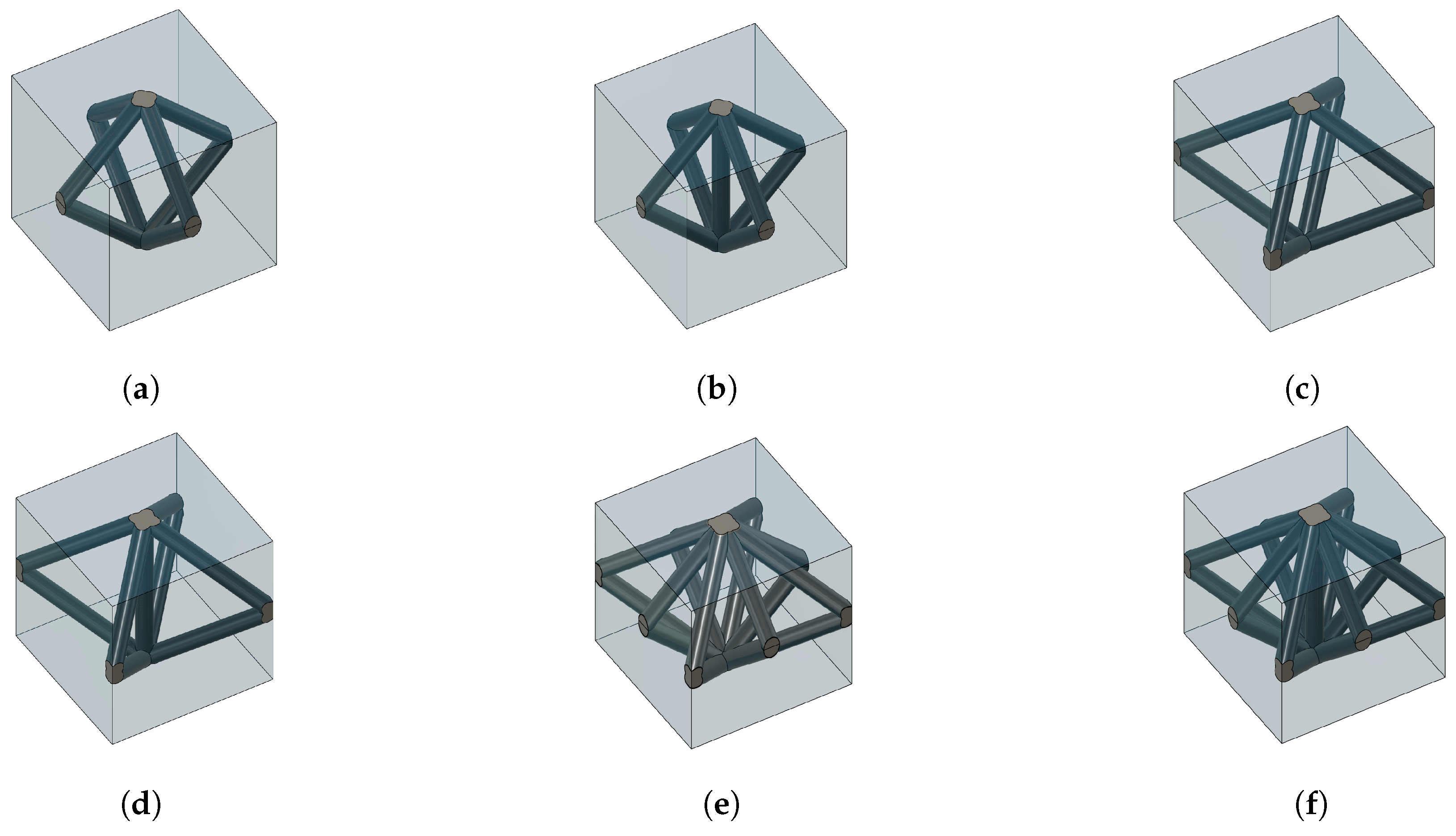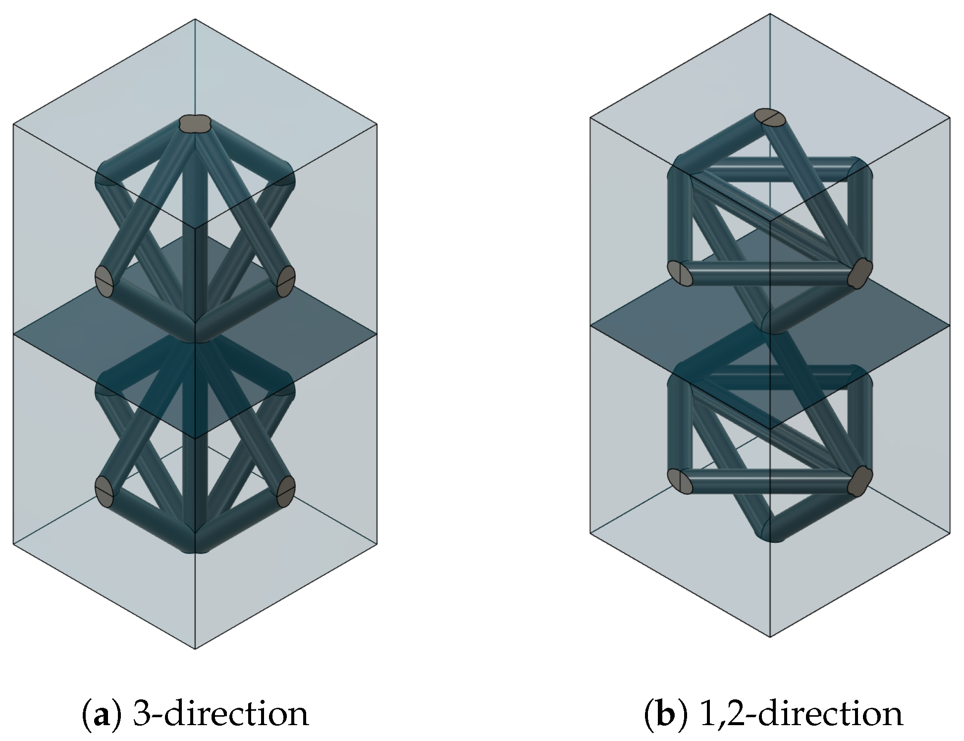Due to their large surface area, such lattices are often investigated for applications such as heat exchangers [5]. The unit cells of strut-based lattices are prismatic, and the struts join different vertices via segments lying either on the face diagonals of the prism (face-centered) or via volume diagonals (body-centered). 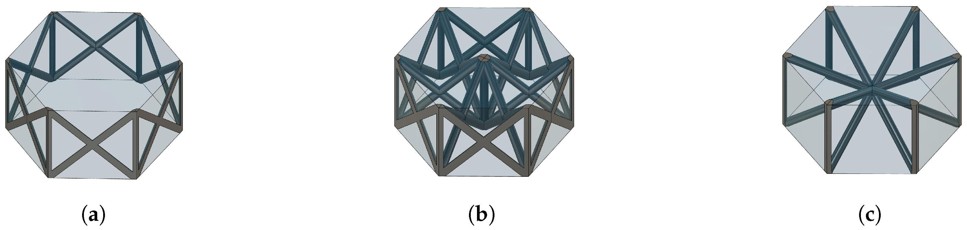A schematic representation of the most common ones is given in Figure 1, while novel unit cells with a hexagonal shape are shown in Figure 2. These are also studied in this work.

These structures can be tailored to exhibit specific geometries and properties, including enhanced thermal conductivity. Moreover, the versatility in design made possible by additive manufacturing techniques enables the fine-tuning of the lattice parameters, such as the strut diameter, strut angle, cell size, porosity, and the overall structural geometry. This fine-tuning aims to maximize the enhancement in thermal conductivity.

Several authors have investigated, both numerically and experimentally, the thermal performance of composites composed of strut-based lattice structures and PCMs. Righetti et al. [6] analyzed the effect of varying cell sizes for different bcc lattice samples with the same porosity. They concluded that the melting time was the lowest for the sample with the smallest cell size. In prior research, the authors of this work empirically demonstrated that the impact of the cell topology on the thermal behavior of the composite is a primary factor. They also found that, in comparison to metal foams, the effect of natural convection on the thermal performance of lattice structure–PCM composites is enhanced. This is mainly attributed to the geometries of some lattice structures, which can exhibit larger pore sizes for the same porosity [7]. While architectured lattice structures are becoming increasingly popular, the description of the effective thermophysical properties has been approached by only a few authors and it still represents a challenge. 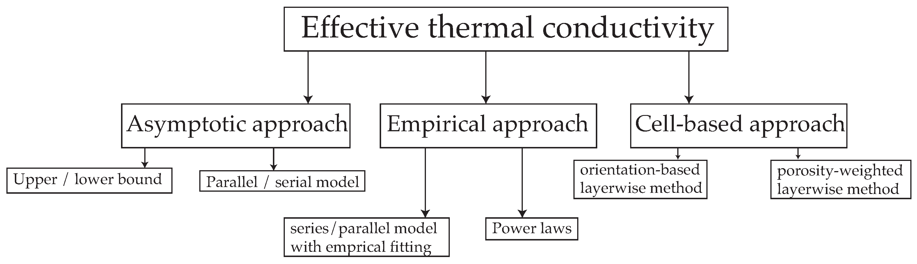The effective density and heat capacity can be determined with the help of simple volumetric mixing laws [8]. However, the effective thermal conductivity is strongly dependent on the geometry of the porous material. The methods to determine the effective thermal conductivity of a lattice structure are similar to the ones developed in the last few decades to describe foams. These can be divided into three categories: asymptotic, empirical, and cell-based approaches [9], as schematically shown in Figure 3.

The asymptotic approach, mainly attributed to Maxwell, univocally relates the effective thermal conductivity to the porosity and sets upper and lower bounds to the effective thermal conductivity. According to Ranut et al. [9], the method is poor in predicting the ETC. However, several authors have adapted this method by using empirical correction factors. Calmidi and Mahajan [10] fitted the parallel model with a coefficient A and an exponential factor n. Bhattachaeya et al. [11] used both parallel and serial models to assess the contribution of each model to the effective thermal conductivity (ETC) of high-porosity metal foams. Mendes et al. [12] examined different methods of calculating the upper bound and lower bound, such as the Hashin–Shtrikman bounds [13] or the effective medium theory, along with a combination of these methods. They obtained good results with certain combinations of the different bound methods. Wang et al. [14] investigated the effective thermal conductivity of sandwich panels based on lattice cores for high-temperature applications and delivered a power law correlation for the effective thermal conductivity. Similarly, several authors have developed correlations based on power laws to describe the effective thermal conductivity for a variety of lattice structures, both with and without PCMs as fillers [15,16,17]. The empirical models demonstrate a high level of accuracy in estimating the effective thermal conductivity (ETC) for various material combinations. Nonetheless, these models exhibit limited flexibility when it comes to accommodating different geometries. For small changes in the matrices, new empirical factors have to be determined to make the equations match reality. To improve the flexibility of ETC models, cell-based approaches were introduced by Calmidi and Mahajan [10] to describe the effective thermal conductivity of metal foams approximating random cells with hexagons. Using this method, the effect of the geometry of the porous medium can be considered. However, due to the randomness of the foam geometry, empirical factors are usually used to adapt the models to the experimental or numerical results. The thermal network method is frequently used to calculate the conductivity of different layers in series. Alternatively, the conductivity can be determined with a porosity-weighted approach [10,18], which does not take into account the strut or the ligament orientation, unlike the strut orientation-based methods [19,20,21]. To model the structure precisely, the ligament orientation needs to be respected, as a longer distance of the ligament leads to higher thermal resistance. Due to the high regularity and periodicity of the geometry of a lattice structure, cell-based models can offer high reliability and robustness to predict the ETC, and they are theoretically superior to purely empirical methods. To the authors’ knowledge, only Hubert et al. [22] have used a cell-based approach to obtain the ETC of a lattice structure with a PCM as a filler. They used fitting coefficients to model the complex intersections between struts and nodes at which struts cross each other. Such coefficients are determined from experimental data and are different for different topologies. The nodes are modeled as cubic elements, with their dimensions determined by the empirical coefficients provided experimentally. The model presented in [22] is capable of modeling the ETC for the $bcc$, $bccz$, $f_{2}cc$, and $f_{2}ccz$ cell topologies, taking into account different porosities and with a fixed aspect ratio of 1. However, the number of investigated cell types is limited. There is a large number of cell topologies and new cell shapes, such as hexagonal cells (Figure 2), which can offer a higher packaging density of struts with respect to cubic unit cells. Furthermore, the model in [22] only applies to cubic cells, i.e. the aspect ratio between edge lengths is 1. Variations in the aspect ratio lead to different strut angles and thus to significant changes in the ETC. This is especially interesting for multifunctional use cases. The aspect ratio, being an additional parameter, enables more flexibility in tailoring the material properties. Additionally, in [22], the idealization of the cell nodes is based only on empirical factors. In this work, instead, a novel model is presented. Generic topological parameters are introduced, which allows one to consider a much wider spectrum of geometries with respect to previous works.

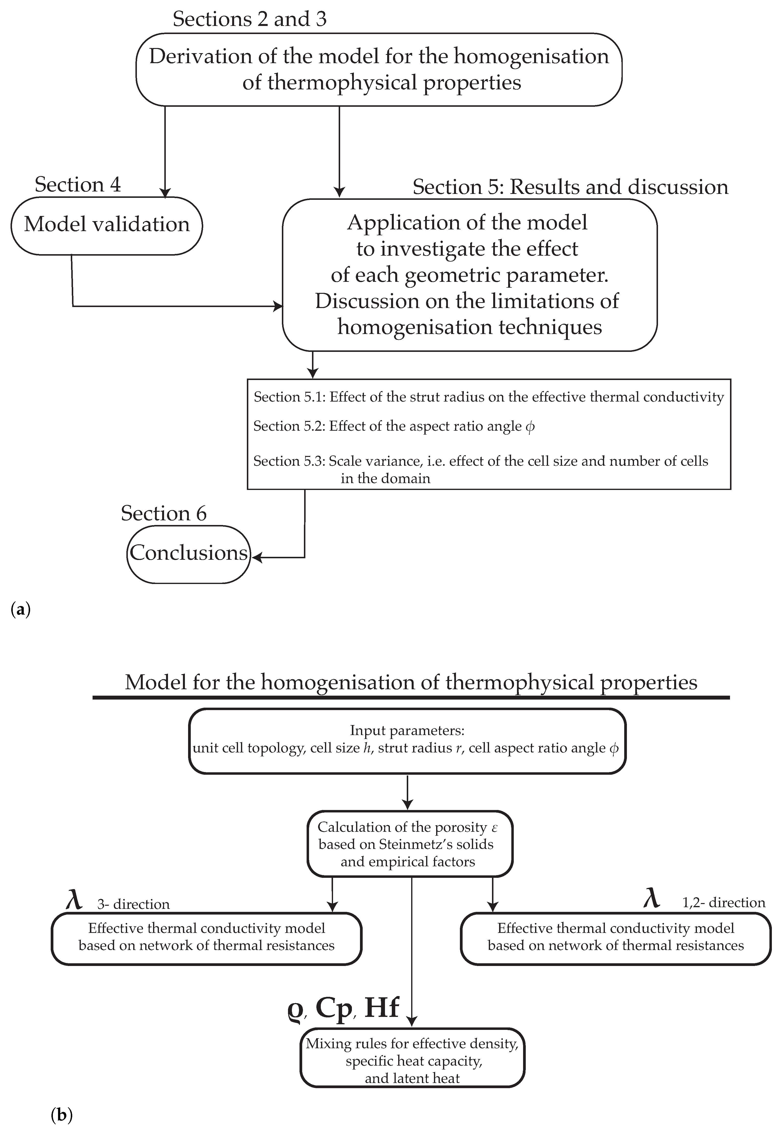
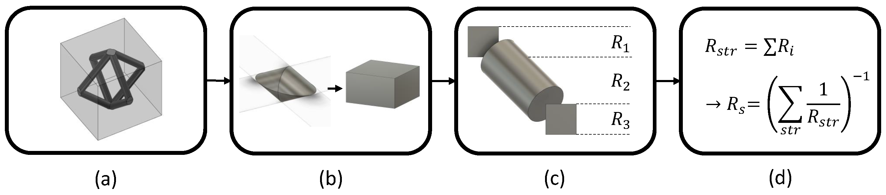
The work is structured as schematically shown in Figure 4. Section 2 focuses on deriving formulae to describe the geometry of the lattice unit cells based on the input parameters (Figure 4b).

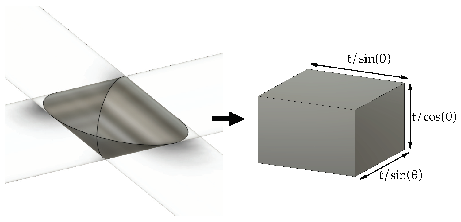
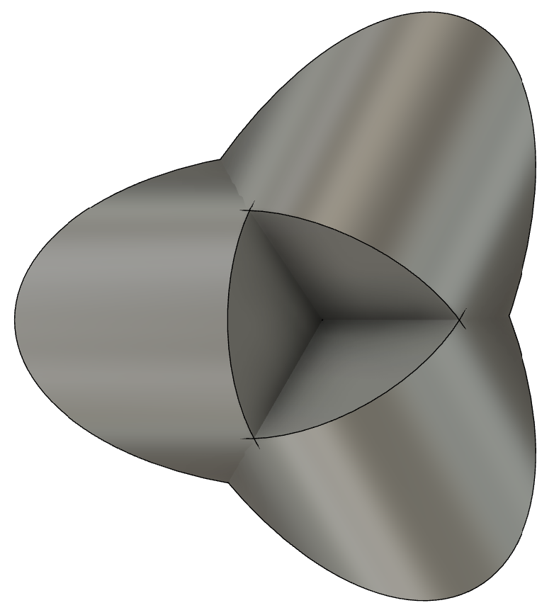
In order to more accurately describe the nodes at the intersection of the struts, Steinmetz’s solids are used [23]. Due to the complex geometry of the cells and in order to account for eventual manufacturing imperfections, the analytical formulae that derive the unit cell porosity are accompanied by empirical factors obtained via numerical investigations. In particular, the model introduced here has the capability to individually analyze the impact of various geometric parameters. These parameters include the cell height, cell aspect ratio (strut angle), strut radius, and cell type. In addition to cubic or parallelepiped unit cells (Figure 1, cells based on hexagonal prisms are treated as well (Figure 2). Although less investigated, such unit cells exhibit the highest packaging density for cylindrical struts in the z direction, which enables the most efficient arrangement of conductive struts for a given porosity. Once the porosity is determined as a function of all the other geometric parameters, the effective thermal conductivity (ETC) can be calculated. The derivation of the ETC, described in Section 3, is based on a network of thermal resistances composed of nodes and struts. The same approach is used to obtain both the ETC in the direction of z struts (3-direction) and in the orthogonal direction (1,2-direction). Simple volume mixing rules are presented in Section 4, where the validation of the presented model is discussed. 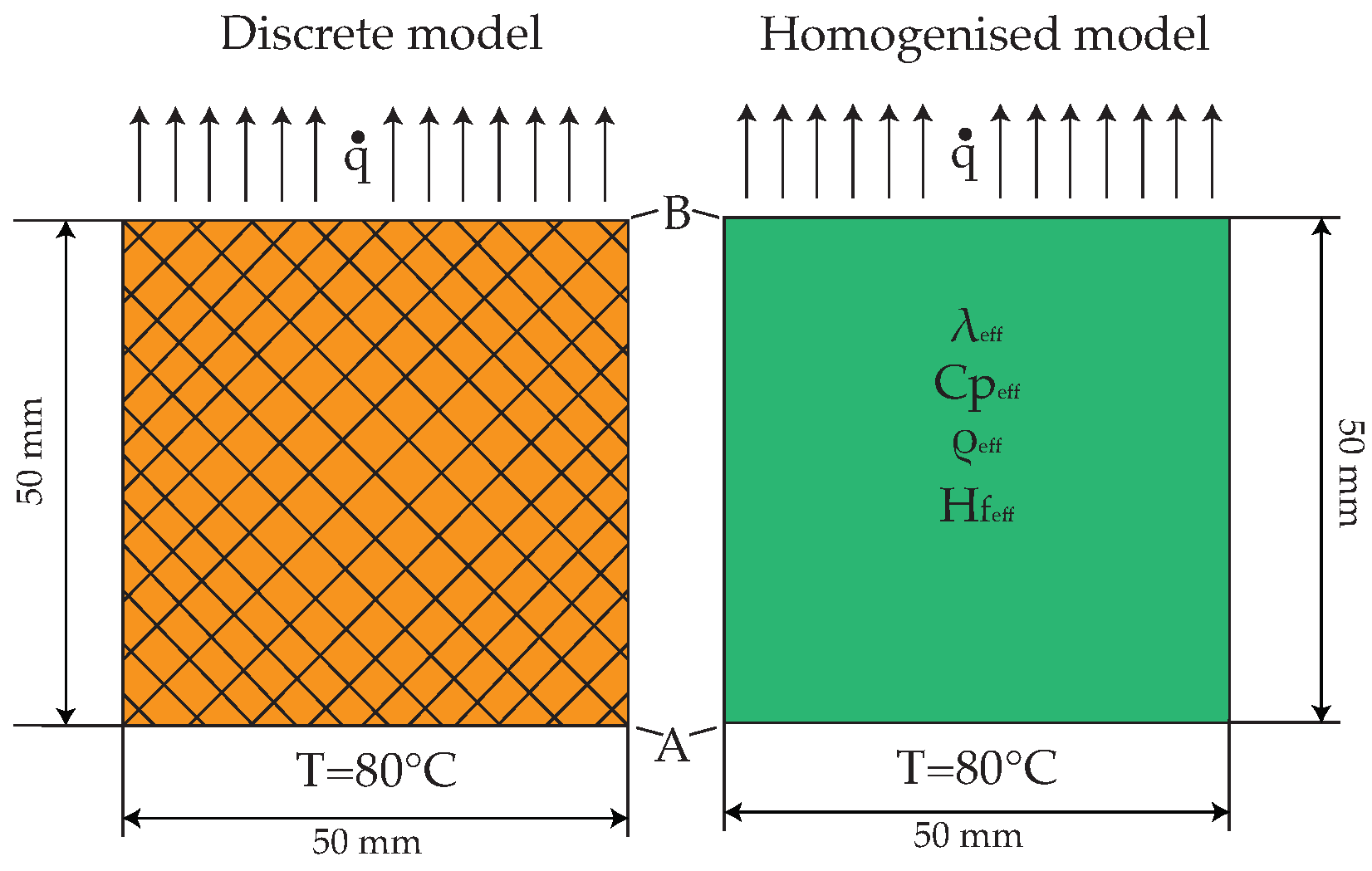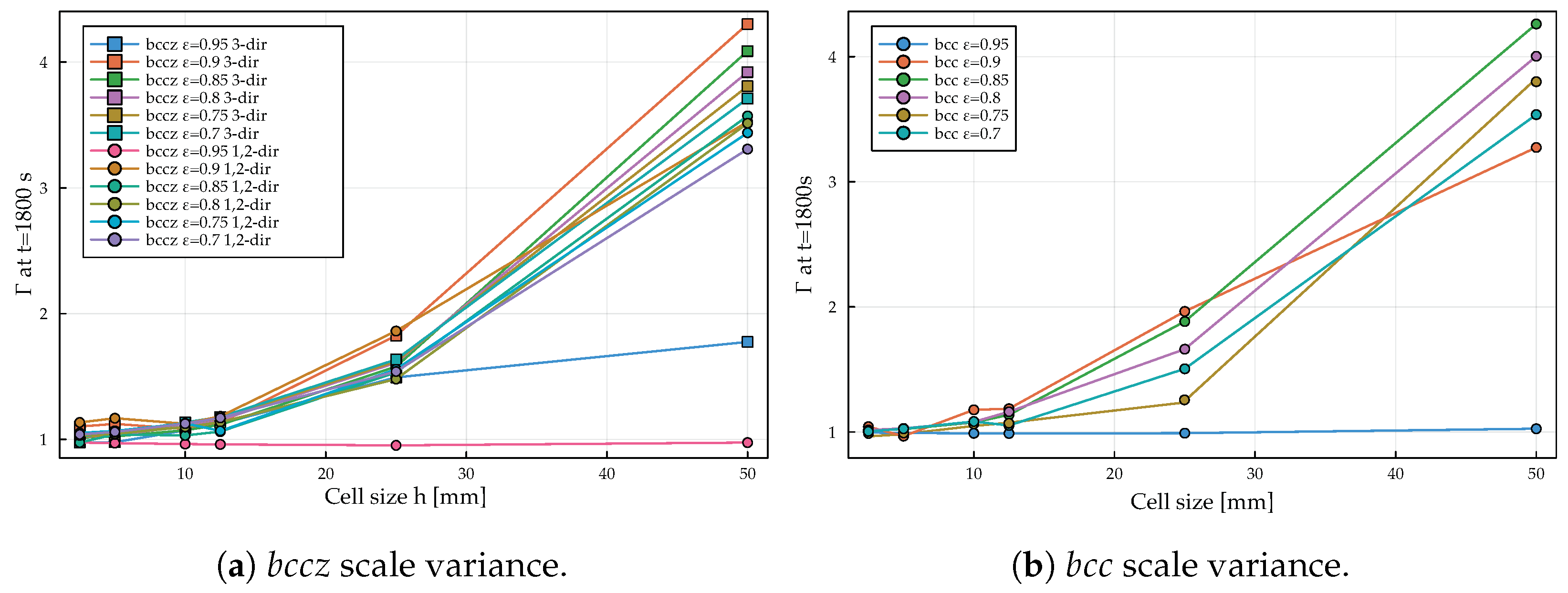Section 5 (Figure 4a) presents an analysis of the quantitative results, with a major focus on the effect of each geometric parameter on the variation in the effective thermal conductivity. Furthermore, the validity of the homogenization techniques, which come with the use of effective thermophysical properties, is discussed. In particular, the scale variance is addressed. According to several authors [12,20], if convection and radiation can be neglected, the ETC of a cellular solid with a filler (e.g., a PCM) can be considered scale-invariant, i.e., a variation in the cell size and strut radius maintaining the same porosity does not lead to a variation in the ETC. While this can be a valid assumption, the transient thermal behavior of the composite is affected by the cell size and by the number of cells present in the domain. Therefore, this work presents the first approach to account for scale variance when treating the composite by means of effective thermophysical properties.

2. Derivation of the Lattice Cell Geometric Properties

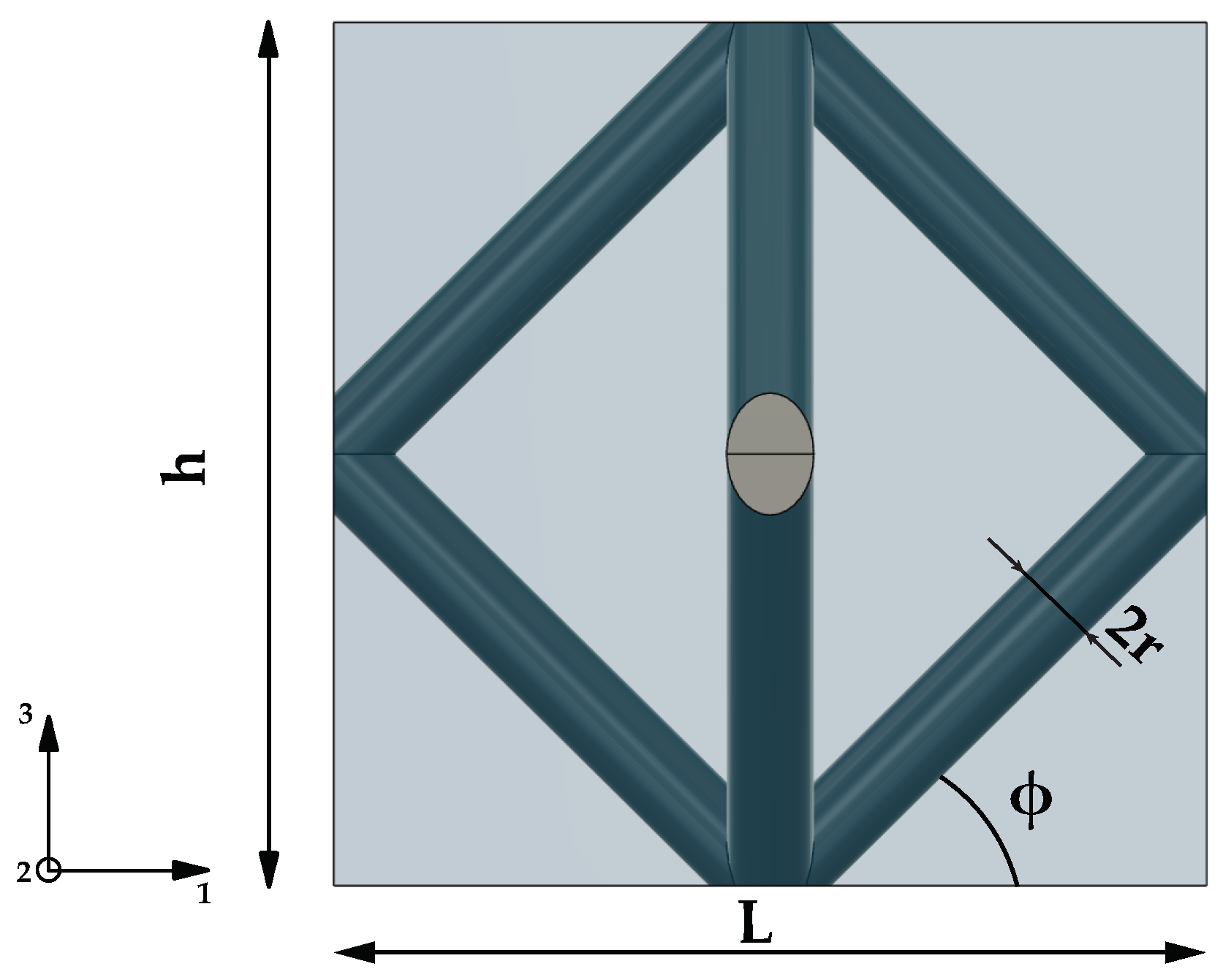
To effectively characterize various cell topologies and make meaningful comparisons between them, it is essential to take into account all geometric parameters within a lattice structure. These variables are the cell height h, the cell width L, the aspect ratio of the cell height h to the cell width L expressed by the angle $\phi =arctan\frac{h}{L}$, the strut radius r, and the cell type. For face-centered (fc) cells, $\phi$ corresponds to the strut angle. For body-centered (bc) cells, the strut angle $\Omega$ follows from Equation (1). For hexagonal cells, $\phi$ corresponds to the ratio of cell height to edge length $L_{side}$. The face-centered struts thus have an angle of $\phi$, while the body-centered strut angle ${\Omega }_{hex}$ is calculated using Equation (2). The following cell types are investigated: $f_{2}cc$, $f_{2}ccz$, $bcc$, $bccz$, $f_{2}bcc$, $f_{2}bccz$, $hpfcz$, $hpbcz$, $tpfcz$. In Figure 5, definitions of the geometric variables of a unit cell are shown.

$$\begin{array}{cc}\hfill \Omega & =arctan\left(tan\left(\phi \right)/\sqrt{2}\right).\hfill \end{array}$$

(1)

$$\begin{array}{cc}\hfill {\Omega }_{hex}& =arctan\left(tan\left(\phi \right)/2\right).\hfill \end{array}$$

(2)

Prior to introducing the analytical models employed in this study, it is pertinent to elucidate their domain of applicability. In order to consider the composite material as a cellular solid infiltrated by a PCM, it is necessary that the unit cells are open on all sides. This condition imposes constraints on the geometric parameters of each individual unit cell. It is important to note that the range of validity varies due to the different topological configurations. 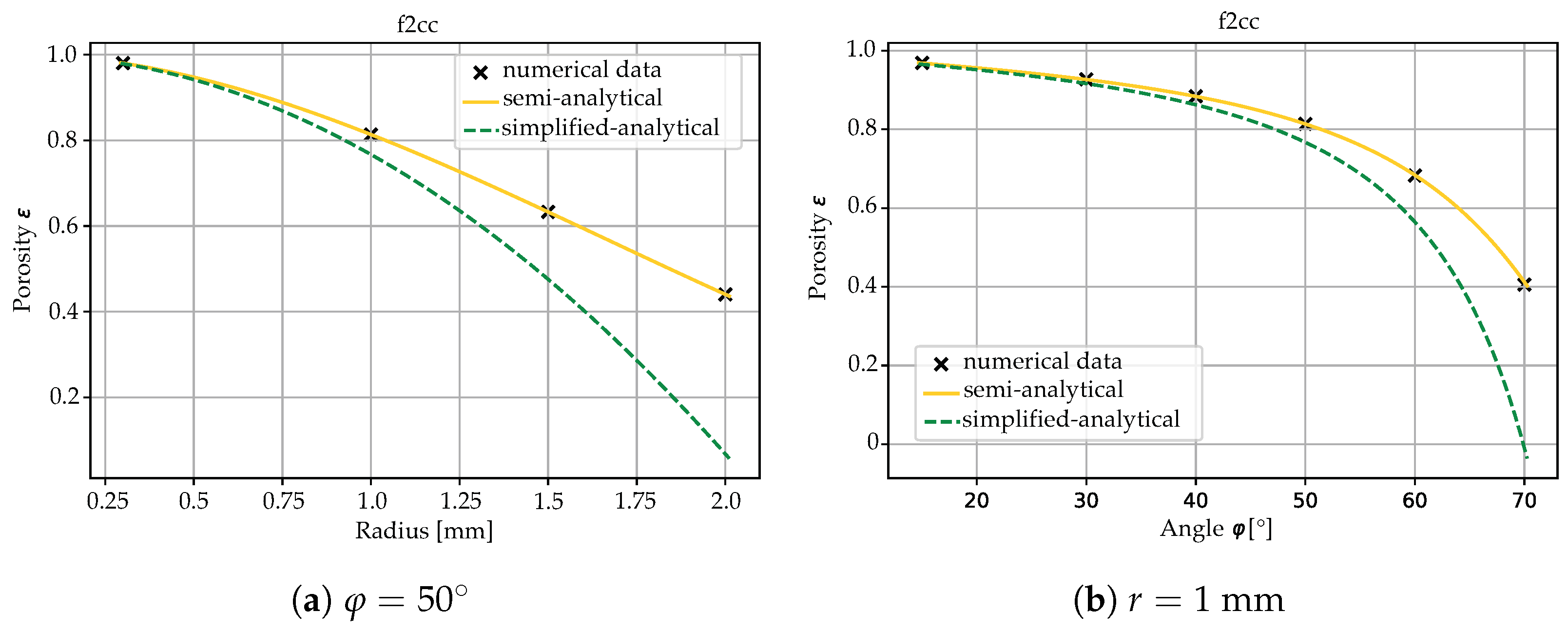For instance, unit cells with a relatively low number of struts, such as the $f_{2}cc$ topology, maintain their status as open cells at porosities below those required for densely packed unit cells, i.e., the $f_{2}bccz$ topology. In summary, the semi-analytical models employed for porosity calculations have been determined to consistently hold true for porosities $\epsilon >0.4$ and aspect ratio angles ${15}^{\circ }<\phi <{75}^{\circ }$. Conversely, the simplified models outlined in Section 3.4 are applicable only when dealing with porosities exceeding 0.9 and aspect ratio angles up to ${45}^{\circ }$. Furthermore, the equations used for the semi-analytical estimation of the ETC exhibit validity within a narrower range of porosities ($\epsilon >0.65$) and aspect ratio angles (${15}^{\circ }<\phi <{65}^{\circ }$). For a comprehensive examination of the scope of validity of the presented models, we refer the reader to Section 4.

2.1. Derivation of the Porosity

For the exact calculation of the ETC, knowledge of the lattice porosity is necessary. The struts are modeled as cylinders. The volume of the cylinder depends on several parameters, introduced in Equation (3). The strut’s length is related to the cell size h and to the strut type, which is taken into account by making use of the strut angle $\vartheta$. The angle $\vartheta$ corresponds to the angle between the horizontal plane (1,2-plane in Figure 5) and the strut. For face-centered (fc) struts, i.e., struts that run across the cell sides, this is the angle $\phi$. For body-centered (bc) struts, which run through the center of the cell, this corresponds to the angle $\Omega$ or ${\Omega }_{hex}$. For z struts, $\vartheta ={90}^{\circ }$.

$$V_{str}\left(\vartheta \right)=\pi r^2\frac{h}{sin\left(\vartheta \right)}$$

(3)

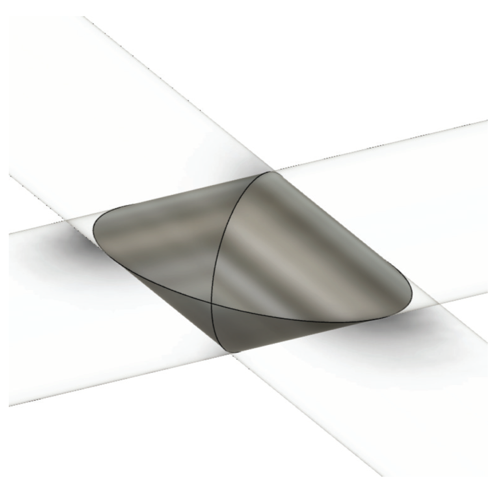
The intersection of two struts creates a generic angle $\alpha$ between the two struts.

Table 1. Value of the angle $\alpha$ for intersections of different types of struts.

Intersection	$\mathit{\alpha }$
2 fc struts	$\pi -2\phi$
2 bc struts	$\pi -2\Omega$
fc and z strut	$\pi /2-\phi$
bc and z strut	$\pi /2-\Omega$

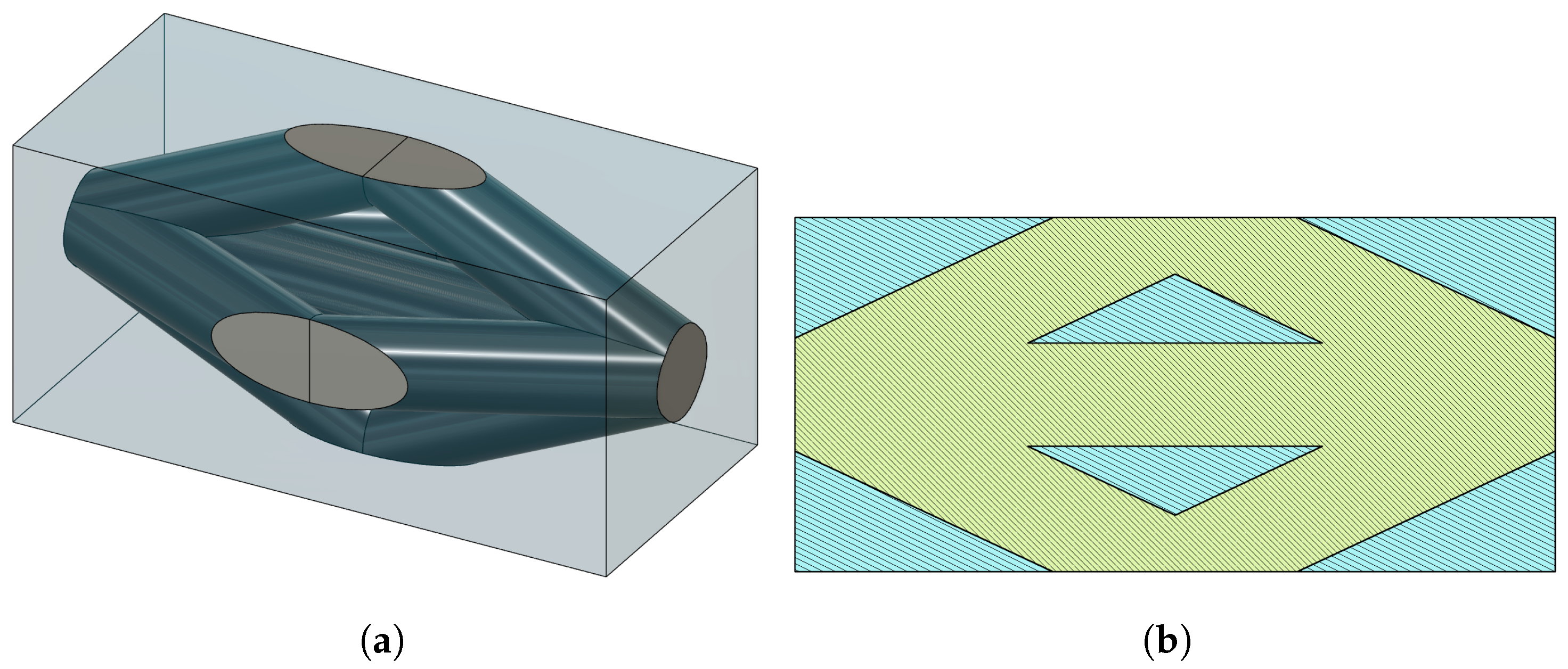
shows the values of $\alpha$ for simple intersections. The volume of the intersection can be described via Steinmetz’s solid, shown in Figure 6. Its volume is

$$V_2\left(\vartheta \right)=\frac{16}{3sin\left(\alpha \right)}{r}^3$$

(4)

Four-fold intersections occur at the top and bottom interfaces of most cells and in the central nodes of body-centered cells. Their volume is calculated according to Equation (5). The equation contains two double intersections from Equation (4), and the overlap between them is subtracted in the last term. The last term corresponds to the volume of a four-fold Steinmetz solid.

$$V_4\left(\vartheta \right)=2V_2\left(\vartheta \right)-12(\sqrt{8}-\sqrt{6})r^3$$

(5)

Eight-fold intersections result from a combination of two four-fold intersections, as indicated in Equation (6). These intersections occur at the interfaces of the cell types $f_{2}bcc$ and $f_{2}bccz$. Here, a body-centered four-fold intersection and a face-centered four-fold intersection are added together for the calculation. The overlap of these two volumes is subtracted from the sum. The subtracted volume can be approximated by a six-fold Steinmetz’s solid, as its volume can be determined analytically and it deviates only slightly from the volume of the eight-fold body [23]. However, as Steinmetz’s solids have analytical solutions only for a constrained amount of intersection angles, the intersection of the fc and bc struts with each other is not taken into account in the subtracting term, leading to inaccuracies that must be corrected with an empirical coefficient.

$$V_8(\phi ,\Omega )=V_{4,bc}(\Omega )+V_{4,fc}\left(\phi \right)-\frac{16}{3}(3+\sqrt{12}-\sqrt{32})r^3$$

(6)

The porosity $\epsilon$ results from the proportion of the lattice volume $V_s$ to the total volume $V_{tot}$ according to Equation (7).

$$\epsilon =\frac{V_{tot}-V_s}{V_{tot}}$$

(7)

The volume fraction $\chi$ is simply the strut volume compared to the total volume and can be calculated from Equation (8).

$$\chi =1-\epsilon =\frac{V_s}{V_{tot}}$$

(8)

The strut volume is calculated via the cylinder volume of a strut together with the number of fc struts, ${\delta }_{fc}$, the number of bc struts, ${\delta }_{bc}$, and the number of z struts, ${\delta }_z$, minus the volumes of the intersections. In general, Equation (9) applies to all cell types. This is composed of Equation (3) with the three different strut types that occur in the cells. The volumes from Equation (4) are subtracted with the respective strut intersection angles that occur.

$$\begin{array}{c}\epsilon =1-\frac{1}{V_{tot}}[\pi r^2{h}_{cell}\left(\frac{{\delta }_{bc}}{sin(\Omega )}+\frac{{\delta }_{fc}}{sin\left(\phi \right)}+{\delta }_z\right)\hfill \\ -\frac{16}{3}{r}^3\left(\frac{F_1}{sin(\pi -2\phi )}+\frac{F_2}{sin(\pi /2-\phi )}+\frac{F_3}{sin(\pi -2\Omega )}+\frac{F_4}{sin(\pi /2-\Omega )}\right)]\end{array}$$

(9)

The first term in the square brackets of Equation (9) models the number of struts with their respective cylinder volumes. The second term subtracts the intersections. The factors $F_1$, $F_2$, $F_3$, and $F_4$ are associated with the number of volumes that need to be subtracted because of the intersection of the struts. The factors can either be derived geometrically or determined empirically. At some intersections, multiple struts cross. In the case of the cell $f_{2}bccz$, for example, nine struts cross at one intersection. This leads to intersection volumes that cannot be determined analytically. Therefore, for such cases, a semi-empirical approach is used to determine the intersection volumes of the struts that need to be subtracted from the cylinder volumes of the struts. The factors $F_i$ are empirically determined and serve as coefficients to adjust or correct the model introduced in this context. The factors $F_1$ and $F_3$ take into account intersections of equal struts. The factors $F_2$ and $F_4$ account for the number of intersections between diagonal struts and z struts.

To obtain an appropriate value of the porosity, the cell topology is accounted for by making use of the coefficients ${\delta }_i$. A $f_{2}ccz$ cell has four fc struts, no bc struts, and a single z strut. Thus, ${\delta }_{bc}=0$ four fc struts ${\delta }_{fc}=4$ and one z strut ${\delta }_z=1$. As $f_{2}ccz$ does not contain bc struts, also the factors $F_3$ and $F_4$ are set to zero. The empirical factors are fitted and evaluated based on the volume measurement functions of CAD-generated geometries. Such factors can be adapted in the future to account for different manufacturing tolerances.

Table 2. Coefficients for the empirical porosity calculation. The RMSE indicates the root mean squared error over the used parameter set.

Cell Type	${\mathit{V}}_{\mathit{tot}}$	${\mathit{\delta }}_{\mathit{bc}}$	${\mathit{\delta }}_{\mathit{fc}}$	${\mathit{\delta }}_{\mathit{z}}$	${\mathit{F}}_1$	${\mathit{F}}_2$	${\mathit{F}}_3$	${\mathit{F}}_4$	RMSE [%]
$f_{2}cc$	$\frac{h_{cell}^3}{{tan}^2\left(\phi \right)}$	0	4	0	3.061	1.954	0	0	0.38
$f_{2}ccz$	$\frac{h_{cell}^3}{{tan}^2\left(\phi \right)}$	0	4	1	2.935	3.667	0	0	0.18
$bcc$	$\frac{h_{cell}^3}{{tan}^2\left(\phi \right)}$	4	0	0	0	0	2.993	3.340	0.13
$bccz$	$\frac{h_{cell}^3}{{tan}^2\left(\phi \right)}$	4	0	1	0	0	3.137	4.923	0.33
$f_{2}bcc$	$\frac{h_{cell}^3}{{tan}^2\left(\phi \right)}$	4	4	1	3.940	4.380	3.706	4.190	0.07
$f_{2}bccz$	$\frac{h_{cell}^3}{{tan}^2\left(\phi \right)}$	4	4	1	3.741	5.874	3.340	4.779	0.61
$hpfcz$	$\frac{3\sqrt{3}{h}_{cell}^3}{2{tan}^2\left(\phi \right)}$	0	6	2	5.133	4.756	0	0	0.98
$hpbcz$	$\frac{3\sqrt{3}{h}_{cell}^3}{2{tan}^2\left(\phi \right)}$	6	0	2	0	0	5.093	8.334	0.18
$tpfcz$	$\frac{3\sqrt{3}{h}_{cell}^3}{2{tan}^2\left(\phi \right)}$	0	18	3	12.907	20.254	0	0	0.28

shows the fitted factors of the respective cells with the numerically obtained volumes. A gradient descent algorithm is used to find appropriate values for the parameters $F_i$. The root mean squared error (RMSE) of the derived equations is shown in Table 2. The empirical fits show very good approximation over a wide porosity range with errors below 1%. The equations can be used for porosities of $\epsilon >0.5$. Once this threshold is reached, the pores created by the cells are no longer open.

3. Effective Thermal Conductivity Model

The effective thermal conductivity depends both on the porosity of the unit cell and on the other geometric parameters. In general, the effective thermal conductivity of a lattice structure is orthotropic; thus, a model is derived for the 3-direction and the 1,2 ones. The following assumptions are made:

• no convection or radiation is present;
• the thermophysical properties remain constant over the temperature interval across a unit cell;
• thermal equilibrium is assumed.

A thermal network is used to calculate the ETC. The network is divided into three layers. The first layer contains the node at the top or bottom cell interface. The second layer covers the strut that connects the two nodes. The third layer contains the second node at the intersection point of the struts, halfway through the cell. To determine the conductivity, the thermal resistance of the individual layers is determined first. The following simplifications are used for the calculation procedure.

• All unit cells are symmetric in all three spatial directions lying on planes that pass through the center point. Thus, such symmetry is exploited to simplify the calculations.
• The thermal resistance of the strut intersections is modeled as a cuboid node (Figure 8). Since the cuboid is obtained as an equivalent volume of Steinmetz’s solid, the number and type of struts (i.e., face-centered or body-centered) that cross at a specific node are important in defining its resistance.
• Only the lattice structure is taken into account. The filler, i.e., PCM, is included as thermal resistance placed in parallel to one of the lattice unit cells.

Figure 7 schematically describes the procedure of deriving the ETC.

3.1. Three-Direction

The edge lengths of the cube representing the intersection nodes result from the strut angle $\vartheta$ and the volume of the struts, as schematically shown in Figure 8. If a bc strut is considered, the angle $\Omega$ is used to calculate the edge length. If a fc strut is used, $\vartheta =\phi$. This procedure is also applied to the eight-fold intersections where both strut types meet at the intersection. The cube is different for every strut type, even if the struts meet at the same intersection. For the calculation of the edge length t of the n-fold intersection of the cube, Equation (10) is obtained.

$$t_n(\vartheta ,V_n)={\left(V_n\left(\vartheta \right){sin}^2\left(\vartheta \right)cos\left(\vartheta \right)\right)}^{1/3}$$

(10)

Thus, for the resistance of the first section, Equation (11) follows:

$$R_1(n,\vartheta )=\frac{n{t}_n/(2cos\left(\vartheta \right))}{{\sigma }_1{t}_n^2/{sin}^2\left(\vartheta \right){\lambda }_s}=\frac{1}{{\sigma }_1}\frac{n{sin}^2\left(\vartheta \right)}{2t_{n}cos\left(\vartheta \right){\lambda }_s}$$

(11)

where n represents the number of struts involved in the intersection. The z strut is not counted. $\sigma$ is an empirical factor introduced to take into account the complex intersections at the nodes. It is assumed that the resistance is reduced by the accumulation of material. ${\lambda }_s$ is the conductivity of the strut material. The same procedure applies to the third layer. Equation (12) calculates the resistance for the third layer at half cell height.

$$R_3(n,\vartheta )=\frac{1}{{\sigma }_3}\frac{n{sin}^2\left(\vartheta \right)}{2t_{n}cos\left(\vartheta \right){\lambda }_s}$$

(12)

A different procedure is used for the second layer. Here, the longitudinal resistance of a cylinder is used. To obtain the new strut length, the distance from the node center to the corner of the node is subtracted from the strut length. Equation (13) follows for the new strut length $L_{str}$.

$$L_{str}(\vartheta ,n_1,n_3)=\frac{h}{2sin\left(\vartheta \right)}-\frac{t_{n_1}(\vartheta ,V_{n_1})+t_{n_3}(\vartheta ,V_{n_3})}{2}{\left(\frac{1}{{cos}^2\left(\vartheta \right)}+\frac{2}{{sin}^2\left(\vartheta \right)}\right)}^{0.5}$$

(13)

With $L_{str}$, we have Equation (14) for the resistance of the second layer.

$$R_2(\vartheta ,n_1,n_3)=\frac{L_{str}(\vartheta ,n_1,n_3)}{\pi r^2{\lambda }_s}$$

(14)

Overall, the resistance through the entire cell of a single strut results from a series system of the individual layer resistances in Equation (15). As only the half strut length is used for the resistances $R_1$, $R_2$, $R_3$, they are multiplied by two to obtain the resistance of a strut through the cell.

$$R_{str}(\vartheta ,n_1,n_3)=2\left(R_1(\vartheta ,n_1)+R_2(\vartheta ,n_1,n_3)+R_3(\vartheta ,n_3)\right)$$

(15)

A simpler model is used for the z strut, which is assumed to pass through the complete cell height. The influence of the accumulation in the nodes is taken into account by the empirical factors $\sigma$ of the other diagonal struts. The overall resistance of the lattice can be calculated from the number of struts together with $R_{str}$. Equation (16) shows the total resistance of the struts.

$$R_s={\left[\frac{{\delta }_{bc}}{R_{str,bc}(\Omega ,n_1,n_3)}+\frac{{\delta }_{fc}}{R_{str,fc}(\phi ,n_1,n_3)}+\frac{{\delta }_z}{R_z}\right]}^{-1}$$

(16)

3.2. One- and Two-Direction

The same approach is used for the ETC in the 1,2-direction. The calculation of the node volumes remains the same. The cell is rotated by 90° around one of the horizontal axes. The layers are divided along the investigated direction (1- or 2-direction). Figure 9 shows the stacked cells in different orientations. In the figure, the cell is rotated around the 2-axis. The volume of the prism at the intersections of the struts changes compared to the modeling in the 3-direction. In the 1,2 direction, the edge length of the prism becomes $t/sin\left(\vartheta \right)$. The guiding surface of the prism corresponds to ${(t/cos\left(\vartheta \right))}^2$. Thus, Equation (17) for the edge length parameter t is obtained.

$$t_n(\vartheta ,V_n)={\left(V_n\left(\vartheta \right)sin\left(\vartheta \right){cos}^2\left(\vartheta \right)\right)}^{1/3}$$

(17)

The resistances of the nodes result from Equation (18) for the node of the first layer and Equation (19) for the node of the third layer.

$$\begin{array}{cc}\hfill R_1(n,\vartheta )& =\frac{1}{{\sigma }_1}\frac{n{cos}^2\left(\vartheta \right)}{2t_{n}sin\left(\vartheta \right){\lambda }_s}\hfill \end{array}$$

(18)

$$\begin{array}{cc}\hfill R_3(n,\vartheta )& =\frac{1}{{\sigma }_3}\frac{n{cos}^2\left(\vartheta \right)}{2t_{n}sin\left(\vartheta \right){\lambda }_s}\hfill \end{array}$$

(19)

Due to the rotation, not all struts contribute efficiently to the conductivity anymore. The z strut in Figure 9b does not connect the bottom and top interfaces of the cell anymore. Nevertheless, these struts improve the conductivity of the cells because the intersections of the nodes become thicker. The additional material increases the conductive surface and reduces the path length, thus lowering the resistance. This influence can be taken into account by the empirical parameter $\sigma$ (Equation (20)).

$${\sigma }_i=\sigma tan\left(\vartheta \right)$$

(20)

The conductivity of layer two is calculated from the same equations for the 3-direction (Equations (13) and (14)), but with the new strut length from Equation (17). The conductivity of the lattice can thus be calculated from Equations (21) and (22). For a $f_{2}bccz$ cell, it thus follows that there are two fc struts (${\delta }_{fc}=2$), since the remaining struts do not contribute directly to the conductivity, four bc struts (${\delta }_{bc}=4$), and zero z-struts (${\delta }_z=0$) per unit cell.

$$\begin{array}{cc}\hfill R_{str}(\vartheta ,n_1,n_3)& =2\left(R_1(\vartheta ,n_1)+R_2(\vartheta ,n_1,n_3)+R_3(\vartheta ,n_3)\right)\hfill \end{array}$$

(21)

$$\begin{array}{cc}\hfill R_s& ={\left[\frac{{\delta }_{bc}}{R_{str,bc}(\Omega ,n_1,n_3)}+\frac{{\delta }_{fc}}{R_{str,fc}(\phi ,n_1,n_3)}\right]}^{-1}\hfill \end{array}$$

(22)

3.3. Cell Topology

3.3.1. Cuboid Prisms

For the cuboid cells (i.e., cubic or parallelepiped with rectangular faces), the ETC can be determined as follows. For example, a cell of type $f_{2}bccz$ has four fc struts (${\delta }_{fc}=4$), four bc struts (${\delta }_{bc}=4$), and one z strut (${\delta }_z=1$) per unit cell. For the strut resistance $R_{str,bc}$, there is an eight-fold intersection in the first layer and a four-fold intersection in the third layer. Thus, $R_{str,bc}(\Omega ,8,4)$ is used. The fc struts have an eight-fold intersection in layer one and a two-fold intersection in layer three. This results in $R_{str,fc}(\phi ,8,2)$. The empirical coefficients are determined numerically. A gradient descent algorithm is used to find accurate values.

Table 3. Coefficients to calculate the ETC in 3-direction for cubic cell types. The RMSE is calculated varying the topological cell setups.

Cell Type	${\mathit{\delta }}_{\mathit{fc}}$	${\mathit{\delta }}_{\mathit{bc}}$	${\mathit{\delta }}_{\mathit{z}}$	${\mathit{n}}_{1,\mathit{fc}}$	${\mathit{n}}_{3,\mathit{fc}}$	${\mathit{n}}_{1,\mathit{bc}}$	${\mathit{n}}_{3,\mathit{bc}}$	${\mathit{\sigma }}_{1,\mathit{fc}}$	${\mathit{\sigma }}_{3,\mathit{fc}}$	${\mathit{\sigma }}_{1,\mathit{bc}}$	${\mathit{\sigma }}_{3,\mathit{bc}}$	RMSE
$f_{2}cc$	4	0	0	4	2	-	-	2.024	1.793	-	-	2.09
$f_{2}ccz$	4	0	1	4	2	-	-	1.448	1.168	-	-	1.65
$bcc$	0	4	0	-	-	4	4	-	-	1.903	1.903	1.59
$bccz$	0	4	1	-	-	4	4	-	-	1.537	1.537	1.85
$f_{2}bcc$	4	4	0	8	2	8	4	2.145	1.311	2.145	1.311	1.01
$f_{2}bccz$	4	4	1	8	2	8	4	1.654	1.185	1.654	1.133	1.00

and

Table 4. Coefficients to calculate the ETC in 1- and 2-direction for cuboid cell types. The RMSE is calculated with different topological cell setups. For this direction, high angles $\phi$ cannot be respected as it leads to large material accumulation at the intersections. For the cells marked with a *, the factor is multiplied by $tan\vartheta$ as in Equation (20).

Cell Type	${\mathit{\delta }}_{\mathit{fc}}$	${\mathit{\delta }}_{\mathit{bc}}$	${\mathit{n}}_{1,\mathit{fc}}$	${\mathit{n}}_{3,\mathit{fc}}$	${\mathit{n}}_{1,\mathit{bc}}$	${\mathit{n}}_{3,\mathit{bc}}$	${\mathit{\sigma }}_{1,\mathit{fc}}$	${\mathit{\sigma }}_{3,\mathit{fc}}$	${\mathit{\sigma }}_{1,\mathit{bc}}$	${\mathit{\sigma }}_{3,\mathit{bc}}$	RMSE
$f_{2}cc$	2	0	4	2	-	-	2.618	3.316	-	-	1.14
$f_{2}ccz$	2	0	4	2	-	-	1.732	2.836	-	-	1.54
$bcc$	0	4	-	-	4	4	-	-	4.277	4.277	1.52
$bccz$	0	4	-	-	4	4	-	-	10.95 *	4.073	1.61
$f_{2}bcc$	4	4	8	2	8	4	10.86 *	2.420	10.86 *	3.840	1.87
$f_{2}bccz$	4	4	8	2	8	4	9.576 *	3.468	9.576 *	4.564	2.38

show the coefficients to be used and values for $\sigma$ for the cuboid cells.

In the 3-direction, the empirical factors $\sigma$ decrease when a z strut is added. This is reasonable because the z strut occupies a fraction of the node of the first layer and the diagonal struts thus have less conducting surface. If $\sigma$ decreases, the resistance of the strut increases. Once the resistance $R_s$ of the lattice is derived, the effective conductivity can be calculated via Equations (23) and (24) with the inputs cell type, radius r, cell height h, and angle $\phi$ of the cell. The conductivity of the filler ${\lambda }_f$ is taken into account, weighted with the porosity $\epsilon$.

$${\lambda }_{ef{f}_3}(\phi ,r,h)=\frac{{tan}^2\left(\phi \right)}{h{R}_s}+\epsilon {\lambda }_f$$

(23)

$${\lambda }_{ef{f}_{1-2}}(\phi ,r,h)=\epsilon {\lambda }_f+\frac{1}{h{R}_s}$$

(24)

3.3.2. Hexagonal Prismatic Cells

The hexagonal prismatic cells $hpfcz$, $tpfcz$, and $hpbcz$ have different types of intersections. A six-fold intersection occurs at the center of the $hpbcz$ cell and at the corners of the $tpfcz$ cell. Thus, three two-fold intersections are combined and the volume of their overlap is subtracted (Equation (25)). The subtracted volume is similar to the volume already subtracted for four-fold intersections. The difference is that the nodes intersect with the angle $\pi /3$ instead of $\pi /2$, so that the subtracted volume is larger.

$$V_6\left(\vartheta \right)=3V_2\left(\vartheta \right)-2\frac{12(\sqrt{8}-\sqrt{6})}{sin(\pi /3)}{r}^3$$

(25)

The volume on the edges requires a different treatment because the struts are not fully compenetrating. Figure 10 shows the intersecting half Steinmetz’s solids. The volume is referred to as a three-fold intersection and can be determined by Equation (26).

$$V_3\left(\vartheta \right)=\frac{3}{2}{V}_2\left(\vartheta \right)-\frac{1}{2}\frac{12(\sqrt{8}-\sqrt{6})}{sin(\pi /3)}{r}^3$$

(26)

The edge length of the cube and the resistances of the layers are calculated according to the previously presented procedure (Equations (10)–(16)). For the cells $hpfcz$ and $tpfcz$, the angle $\phi$ shall be used for the struts. For the cell $hpbcz$, the angle ${\Omega }_{hex}$ is considered. Equation (27) follows for the effective conductivity in the 3-direction of the hexagonal cells.

$${\lambda }_{ef{f}_3}(\phi ,r,h)=\frac{2{tan}^2\left(\phi \right)}{3\sqrt{3}h{R}_s}+\epsilon {\lambda }_f$$

(27)

Table 5. Coefficients to calculate the ETC in 3-direction for hexagonal cell types. The RMSE is calculated with different topological cell setups.

Cell Type	${\mathit{\delta }}_{\mathit{fc}}$	${\mathit{\delta }}_{\mathit{bc}}$	${\mathit{\delta }}_{\mathit{z}}$	${\mathit{n}}_{1,\mathit{fc}}$	${\mathit{n}}_{3,\mathit{fc}}$	${\mathit{n}}_{1,\mathit{bc}}$	${\mathit{n}}_{3,\mathit{bc}}$	${\mathit{\sigma }}_{1,\mathit{fc}}$	${\mathit{\sigma }}_{3,\mathit{fc}}$	${\mathit{\sigma }}_{1,\mathit{bc}}$	${\mathit{\sigma }}_{3,\mathit{bc}}$	RMSE
$hpfcz$	6	0	2	3	2	-	-	1.027	1.803	-	-	1.27
$tpfcz$	18	0	3	6	2	-	-	1.671	1.178	-	-	2.75
$hpbcz$	0	6	2	-	-	3	6	-	-	1.484	1.754	2.93

shows the parameters to be used for the different cell types.

The edge length of the nodes is calculated using Equation (17), while the resistances of the first and third layers are calculated using Equations (18) and (19). The second layer is calculated using Equations (13) and (14). Setting up the total resistance in the 1,2-direction of the struts requires a different approach for the hexagonal cells. For the $hpfcz$ cell, two total strut lengths are needed to pass from one side of the hexagon to the other. Two strut paths effectively lead from the top to bottom interface. For the $tpfcz$ cell, two struts are needed as well, which have six different paths. In the $hpbcz$ cell, four struts conduct directly through the hexagon. Due to the obvious assumption that one strut is composed of two half struts, Equations (28)–(30) follow for the thermal resistances in the 1,2-directions of the struts for the cells $hpfcz$, $tpfcz$, and $hpbcz$, respectively.

$$\begin{array}{cc}\hfill R_{s,hpfcz}& =\frac{1}{2}4\left(R_1+R_2+R_3\right),\hfill \end{array}$$

(28)

$$\begin{array}{cc}\hfill R_{s,tpfcz}& =\frac{1}{6}4\left(R_1+R_2+R_3\right),\hfill \end{array}$$

(29)

$$\begin{array}{cc}\hfill R_{s,hpbcz}& =\frac{1}{4}2\left(R_1+R_2+R_3\right).\hfill \end{array}$$

(30)

Equation (31) follows for the ETC of the hexagonal cells in the 1,2-direction. All coefficients to calculate the ETC are summarized in

Table 6. Coefficients to calculate the ETC in 1- and 2-direction for hexagonal cell types. The RMSE is calculated with different topological cell setups. For this direction, high angles $\phi$ cannot be respected as it leads to large material accumulation at the intersections. For the cells marked with a *, the factor is multiplied by $tan\vartheta$ as in Equation (20).

Cell Type	${\mathit{\delta }}_{\mathit{fc}}$	${\mathit{\delta }}_{\mathit{bc}}$	${\mathit{n}}_{1,\mathit{fc}}$	${\mathit{n}}_{3,\mathit{fc}}$	${\mathit{n}}_{1,\mathit{bc}}$	${\mathit{n}}_{3,\mathit{bc}}$	${\mathit{\sigma }}_{1,\mathit{fc}}$	${\mathit{\sigma }}_{3,\mathit{fc}}$	${\mathit{\sigma }}_{1,\mathit{bc}}$	${\mathit{\sigma }}_{3,\mathit{bc}}$	RMSE
$hpfcz$	2/2	0	3	2	-	-	2.815	2.483	-	-	2.5
$tpfcz$	6/2	0	6	2	-	-	8.880 *	2.584	-	-	1.81
$hpbcz$	0	4	-	-	3	6	-	-	8.080 *	8.192	2.86

.

$${\lambda }_{ef{f}_{1,2}}(\phi ,r,h)=\epsilon {\lambda }_f+\frac{2\sqrt{3}}{3h{R}_s}$$

(31)

3.4. Simplified Models

The derived equations of Section 2.1 and Section 3 are valid across a broad range of parameters. Above all, porosity plays a decisive role. As the porosity decreases, the degree of strut overlap increases. This makes the modeling complex and thus necessitates the use of empirical correlation factors in order to accurately describe the geometric and thermal model. With high porosities, on the other hand, the overlaps are small, so a simplification of the model is reasonable. In this case, the general Equation (9) for the porosity yields the simplified formulation in Equation (32). The minimum porosity for which the simplified modeling is widely applicable is $\epsilon =0.9$. Neglecting the overlaps simplifies also the derivation of the ETC, which is provided in

Table 7. Simplified analytical equations to calculate the ETC in 3-direction.

Cell Type	${\mathit{\delta }}_{\mathit{fc}}$	${\mathit{\delta }}_{\mathit{bc}}$	${\mathit{\delta }}_{\mathit{z}}$	ETC
$f_{2}cc$	4	0	0	${\lambda }_{eff}=\epsilon {\lambda }_f+{\lambda }_s{tan}^2\left(\phi \right)\pi \frac{r^2}{h^2}4sin\left(\phi \right)$
$f_{2}ccz$	4	0	1	${\lambda }_{eff}=\epsilon {\lambda }_f+{\lambda }_s{tan}^2\left(\phi \right)\pi \frac{r^2}{h^2}\left(4sin\left(\phi \right)+1\right)$
$bcc$	0	4	0	${\lambda }_{eff}=\epsilon {\lambda }_f+{\lambda }_s{tan}^2\left(\phi \right)\pi \frac{r^2}{h^2}4sin(\Omega )$
$bccz$	0	4	1	${\lambda }_{eff}=\epsilon {\lambda }_f+{\lambda }_s{tan}^2\left(\phi \right)\pi \frac{r^2}{h^2}\left(4sin(\Omega )+1\right)$
$f_{2}bcc$	4	4	0	${\lambda }_{eff}=\epsilon {\lambda }_f+{\lambda }_s{tan}^2\left(\phi \right)\pi \frac{r^2}{h^2}\left(4sin\left(\phi \right)+4sin(\Omega )\right)$
$f_{2}bccz$	4	4	1	${\lambda }_{eff}=\epsilon {\lambda }_f+{\lambda }_s{tan}^2\left(\phi \right)\pi \frac{r^2}{h^2}\left(4sin\left(\phi \right)+4sin(\Omega )+1\right)$
$hpfcz$	6	0	2	${\lambda }_{eff}=\epsilon {\lambda }_f+2\frac{2\pi r^{2}tan{\phi }^2{\lambda }_s}{3\sqrt{3}{h}^2}+6\frac{2\pi r^{2}tan{\phi }^2{\lambda }_s}{3\sqrt{3}{h}^2}sin\phi$
$tpfcz$	18	0	3	${\lambda }_{eff}=\epsilon {\lambda }_f+3\frac{2\pi r^{2}tan{\phi }^2{\lambda }_s}{3\sqrt{3}{h}^2}+18\frac{2\pi r^{2}tan{\phi }^2{\lambda }_s}{3\sqrt{3}{h}^2}sin\phi$
$hpbcz$	0	6	2	${\lambda }_{eff}=\epsilon {\lambda }_f+2\frac{2\pi r^{2}tan{\phi }^2{\lambda }_s}{3\sqrt{3}{h}^2}+6\frac{2\pi r^{2}tan{\phi }^2{\lambda }_s}{3\sqrt{3}{h}^2}sin{\Omega }_{hex}$

and

Table 8. Simplified analytical equations to calculate the ETC in 1- and 2-direction.

Cell Type	${\mathit{\delta }}_{\mathit{fc}}$	${\mathit{\delta }}_{\mathit{bc}}$	${\mathit{\delta }}_{\mathit{z}}$	ETC
$f_{2}cc$	2	0	0	${\lambda }_{eff}=\epsilon {\lambda }_f+{\lambda }_s\pi \frac{r^2}{h^2}2sin\left(\phi \right)$
$f_{2}ccz$	2	0	0	${\lambda }_{eff}=\epsilon {\lambda }_f+{\lambda }_s\pi \frac{r^2}{h^2}2sin\left(\phi \right)$
$bcc$	0	4	0	${\lambda }_{eff}=\epsilon {\lambda }_f+{\lambda }_s\pi \frac{r^2}{h^2}4sin(\Omega )$
$bccz$	0	4	0	${\lambda }_{eff}=\epsilon {\lambda }_f+{\lambda }_s\pi \frac{r^2}{h^2}4sin(\Omega )$
$f_{2}bcc$	2	4	0	${\lambda }_{eff}=\epsilon {\lambda }_f+{\lambda }_s\pi \frac{r^2}{h^2}\left(2sin\left(\phi \right)+4sin(\Omega )\right)$
$f_{2}bccz$	2	4	0	${\lambda }_{eff}=\epsilon {\lambda }_f+{\lambda }_s\pi \frac{r^2}{h^2}\left(2sin\left(\phi \right)+4sin(\Omega \right)$
$hpfcz$	2/2	0	0	${\lambda }_{eff}=\epsilon {\lambda }_f+{\lambda }_s\frac{2\sqrt{3}\pi r^{2}sin\left(\phi \right)}{3h^2}$
$tpfcz$	6/2	0	0	${\lambda }_{eff}=\epsilon {\lambda }_f+3{\lambda }_s\frac{2\sqrt{3}\pi r^{2}sin\left(\phi \right)}{3h^2}$
$hpbcz$	0	6	0	${\lambda }_{eff}=\epsilon {\lambda }_f+4{\lambda }_s\frac{2\sqrt{3}\pi r^{2}sin(\Omega )}{3h^2}$

.

$$\epsilon =1-\frac{1}{V_{tot}}\pi r^2{h}_{cell}\left(\frac{{\delta }_{bc}}{sin(\Omega )}+\frac{{\delta }_{fc}}{sin\left(\phi \right)}+{\delta }_z\right)$$

(32)

4. Validation

4.1. Porosity

Figure 11 shows the derived functions for the porosity with the numerical values obtained from a CAD model. As the semi-analytical equations are calibrated with empirical coefficients obtained from the CAD model, they obviously show very high accuracies and almost no deviation from the numerical results. The simplified model equations have a limited range of validity. Starting from porosities below 0.85, deviations of more than 5% occur. This deviation results from neglecting the Steinmetz’s solids. The more overlaps that occur within the cell, the higher the underestimation of the porosity. Consequently, the porosity is always underestimated by the simplified equations. The simplified model is therefore only viable for cells with porosities $\epsilon >0.9$. The semi-analytical equations are valid for porosities from $\epsilon >0.5$ and angles ${15}^{\circ }<\phi <{75}^{\circ }$.

4.2. Effective Thermal Conductivity

To determine the empirical factors, numerical models based on the Finite Element Method are employed. Furthermore, a validation procedure is conducted, involving a comparison between the outcomes generated by these computational models and the empirical data presented in the model developed by Hubert et al. [22]. Additionally, the current model is assessed by comparing it to experimental results obtained in previous research by the same authors [7].

4.2.1. Finite Element Model

The numerical models are built with the help of the commercial software COMSOL Multiphysics^®. The assumption is made that the only relevant heat transfer mode is heat conduction. A stationary and a transient model are developed. The stationary model is used to determine the ETC. The transient model is used to investigate the time-dependent behavior of the composite PCM and the effect of the cell size on it.

In the stationary model, the material properties are assumed to be constant over the investigated range. To limit the computational effort, a quarter of the cell cross-section is used. As shown before, the cells are symmetrical through the center point so that the cell is fully represented. Hubert et al. [22] have already demonstrated that this assumption is valid. In this approach, several cells are stacked on top of each other. A minimum of seven cells delivers stable results, i.e., an increase in the number of stacked cells does not lead to a variation in the ETC. Figure 12a shows the simulation model and Figure 12b shows the applied boundary conditions for it. The central unit cell is selected as the location for the measurement of the temperature difference, which is used to determine the conductivity. By means of Equation (33), the ETC of a cell can be determined.

$${\lambda }_{eff}=\frac{\dot{q}h}{T_2-T_1}$$

(33)

In Equation (33), $\dot{q}$ is the heat flux flowing through the cell, h is the cell size, $T_1$ is the temperature at the top interface of the cell, and $T_2$ is the temperature at the bottom interface.

Figure 12. Simulation model for the calculation of the ETC and the applied boundary conditions, with a constant value of $\dot{q}$.

Figure 12. Simulation model for the calculation of the ETC and the applied boundary conditions, with a constant value of $\dot{q}$.

A convergence analysis is carried out for each cell. The maximum element size of 1.82 mm and minimum element sizes of 0.078 mm for the cell dimensions $h=10$ mm and $\phi ={45}^{\circ }$ were found to deliver an error $<0.1\%$. The number of elements required depends on the cell complexity. In each case, the smallest radius examined is used for the cells, since this case requires the highest number and smallest size of elements for an accurate calculation. Figure 13 shows the convergence plot for the cell $f_{2}bccz$.

4.2.2. Three-Direction

To validate the equations derived for the ETC in the 3-direction, both numerical results and literature data from [7,22] are used. Figure 14 shows the results of the derived equations, which are compared to the numerical results. However, since Hubert et al. [22] only provide a solution for the cells $f_{2}cc$, $f_{2}ccz$, $bcc$, and $bccz$ with an angle of $\phi ={45}^{\circ }$, the model is only compared in a few plots. The equations are validated for the parameter range ${15}^{\circ }<\phi <{65}^{\circ }$ and $0.01<r/h<0.13$. In general, the equations are valid for porosities $\epsilon >0.65$. Since the applications of the structures mainly target high porosities, this range is suitable for the characterization of the composite.

The simple analytical equations are also plotted in Figure 14. They show good agreement with the experiments for the aspect ratio angle $\phi ={45}^{\circ }$. The conductivity of the cells with bc struts is generally underestimated at this angle. The cells with fc struts are overestimated. As the angle increases, the inaccuracy of the analytical model becomes significantly higher. With higher angles, the ETC is generally overestimated. For small angles, the equations underestimate the ETC. This is due to the overlap of the struts at the cell interfaces.

4.2.3. One- and Two-Direction

The comparison of the derived equations with the numerical results in the 1,2-direction can be seen in Figure 15. In general, good agreement of the analytical results with the numerical ones can be seen. However, the equations have difficulties in predicting the conductivity for high angles (>${60}^{\circ }$). This is due to the struts that are not directly involved in conducting the heat in the 1- and 2-direction, such as the z struts. At high angles, the struts significantly shorten the conduction path and lead to large material accumulation; see Figure 16. However, this is not taken into account in the equations. The semi-analytical equations can therefore only be used for angles $\phi <{60}^{\circ }$. In this parameter range, the equations are accurate, with errors below 5% for porosities above $\epsilon >0.65$. The simple analytical models quickly deviate from the numerical results.

Additionally, the presented equations are validated against experimental results present in the literature. For such purpose, a homogenized composite is considered. The other effective properties are obtained via mixture laws:

$${\rho }_{eff}=\epsilon {\rho }_{PCM}+\chi {\rho }_s$$

(34)

$$C_{p_{eff}}=\epsilon {\displaystyle \frac{{\rho }_{PCM}}{{\rho }_{eff}}}{C}_{p_{PCM}}+\chi {\displaystyle \frac{{\rho }_s}{{\rho }_{eff}}}{C}_{p_s}$$

(35)

$$H_{f_{eff}}=\epsilon {\displaystyle \frac{{\rho }_{PCM}}{{\rho }_{eff}}}{H}_{f_{PCM}}$$

(36)

where $\rho$ is the density, $\epsilon$ is the porosity of the lattice, $\chi$ is its volume fraction, $C_p$ is the specific heat capacity, and $H_f$ is the latent heat of fusion. The effective thermal conductivity is obtained with the model presented in this work. The lattice geometric properties are the ones provided in the previous work [7] and summed up in

Table 9. Unit cell geometries considered for experimental validation based on [7].

	${\mathit{f}}_2\mathit{ccz}$	$\mathit{bccz}$
Cell size	5 mm	5 mm
Radius	1 mm	1 mm
$\phi$	45°	45°

. Using the aforementioned parameters, a homogenized PCM composite is simulated. The energy equation for the PCM is solved using the apparent heat capacity method, implemented in COMSOL^® Multiphysics. Figure 17 shows two plots where the $f_{2}ccz$ and the $bccz$ unit cells are validated against experimental results at a heating orientation opposite to gravity, so that the influence of natural convection can be neglected. While the maximum deviation amounts to 8.58%, this can be attributed to the approximation introduced by the apparent heat capacity method, rather than an error in the calculation of the thermophysical properties.

5. Results and Discussion

The presented semi-analytical ETC model, together with the mixture laws, enables the homogenization of the thermophysical properties of the composite PCM. This in turn facilitates the detailed investigation of the effect of a wide variety of geometric parameters on the thermal behavior of the composite. This section is dedicated to the investigation of such an effect, isolating each parameter from the others.

5.1. Strut Radius

In Figure 18, the effective thermal conductivity in the 3- and in 1,2-directions for all considered unit cells at varying porosity is shown. The effective thermal conductivity (${\lambda }_{eff}$) is normalized against the bulk material from which the lattice structure is made (${\lambda }_s$). A variation in porosity can be obtained by varying any of the geometric parameters while keeping the others constant. For the case shown in Figure 18, the unit cell size is fixed at 5 mm and the angle $\phi$ is kept at 45°, thus maintaining a cubic or regular hexagonal prismatic unit cell.

Figure 18 shows that, clearly, unit cells exhibiting struts in the 3-direction (z struts) are also the ones that exhibit the highest effective thermal conductivity in this direction. Face-centered unit cells for both cuboids and hexagonal prisms exhibit the highest thermal conductivity in the 3-direction. Body-centered unit cells exhibit the lowest thermal conductivity. Body-centered struts have a smaller strut angle $\Omega$ than face-centered ones with the same aspect ratio. Thus, due to the resulting longer struts, represented by space diagonals instead of face diagonals, the cells with predominantly body-centered struts perform worse than the cells with face-centered struts. For the 1,2-direction, different conclusions can be made. The gap between the effective thermal conductivity of one unit cell and the next is reduced as the z struts are ineffective in this direction. In this case, face-centered cells with z struts exhibit the lowest effective thermal conductivity, while body-centered ones demonstrate the highest effective thermal conductivity. The cells with a smaller number of struts and fewer intersecting struts at the nodes, i.e., $f_{2}cc$ and $bcc$, overtake the previously better-conducting cells with decreasing porosity. This can be explained by the fact that the struts overlap more in the cells with many struts as the radius increases and the conductivity no longer increases as effectively. The $hpfcz$ cell has an advantage over the $f_{2}ccz$ cell. Although both cells have the same strut types, the ratio of z struts to fc struts is higher in the $hpfcz$ cell (${\delta }_z/{\delta }_{fc}=1/4$ to ${\delta }_z/{\delta }_{fc}=2/6$). In addition, the number of intersecting struts at the nodes of the top and bottom cell interfaces is lower for $hpfcz$. This also explains the lower ETC for the $tpfcz$ cell. This cell has a ratio ${\delta }_z/{\delta }_{fc}=3/18$, the lowest of the three hexagonal cells, and the struts at the interfaces meet with seven other struts.

5.2. Effect of Aspect Ratio (Angle $\phi$)

Figure 19 shows the effect of varying the angle $\phi$ for the $f_{2}ccz$ unit cell. At high porosity, high values of $\phi$ are beneficial to the ETC. The trend is reversed for decreasing porosity. The accumulation of material at the strut nodes becomes ever more relevant with decreasing porosity. A low value of $\phi$ increases the material accumulation for a given porosity. When the porosity is high, material accumulation at the nodes plays a marginal role and the heat conduction path is shortened if the angle $\phi$ is increased. Cells with a high ${\delta }_z$ to ${\delta }_{fc/bc}$ ratio and high strut angles achieve high ETC at high porosity. Figure 20 and Figure 21 show the effect of $\phi$ for all considered cells in a range of different porosities obtained by keeping the cell size h fixed at 5 mm and varying the strut radius r. The porosity corresponding to each angle and strut radius combination is reported as a dashed line. In Figure 20, the ETC in the 3-direction is reported for strut radii r = 0.1, 0.2, 0.3 mm, respectively. The variation in the angle $\phi$ at a constant strut radius implies porosity variations. One can notice that the lowest ETC is obtained for the cells in which the variation in $\phi$ has the least effect on the porosity of the unit cell. However, as shown in Figure 21 for the 1,2-direction, exceptions can be noticed for cells that exhibit few intersections.

5.3. Scale Variance: Effect of Cell Size and Number of Cells

The cell size has no direct effect on the effective thermal conductivity. If the cell size is increased, keeping the porosity constant, i.e., by accordingly increasing the strut radius, the effective thermal conductivity is not affected, as evident from Figure 22. Here, the cell size of each unit cell is varied in a range between 5 and 30 mm, while the strut radius is accordingly varied between 0.5 and 3 mm, respectively. The porosity of each cell is reported in

Table 10. Porosity of the unit cells considered in the stationary case, with cell size ranging from 5 to 30 mm and radius from 0.5 to 3 mm.

	${\mathit{f}}_2\mathit{cc}$	${\mathit{f}}_2\mathit{ccz}$	$\mathit{bcc}$	$\mathit{bccz}$	${\mathit{f}}_2\mathit{bcc}$	${\mathit{f}}_2\mathit{bccz}$	$\mathit{hpfcz}$	$\mathit{hpbcz}$	$\mathit{tpfcz}$
$\epsilon$	0.85	0.83	0.82	0.80	0.71	0.68	0.90	0.84	0.74

. The result shown in Figure 22 is in good agreement with results presented in the literature regarding the effect of the cell size for metal foams [12,20].

However, while the values obtained correctly predict the effective thermophysical properties, this is not sufficient to describe the transient behavior of a composite made of a PCM and a cellular solid. In particular, lattice structures manufactured via additive manufacturing or investment casting can be designed with a wide range of cell sizes. In realistic applications, both the cell size and the number of cells can be changed depending on a variety of boundary conditions, especially if the volume of a system is constrained. Thus, it is relevant to investigate the effect of the scale variance on the transient thermal behavior of such systems. To do so, a numerical investigation is performed. Both a discrete model and a homogenized one are generated and tested under the same boundary conditions, as schematically sketched in Figure 23. A range of geometric parameters are varied for all considered cells.

With reference to Figure 23, the value of $\dot{q}$ is 1000 W/m${}^2$ and represents one boundary condition for the numerical problem. The other boundary condition is on the opposite side of the domain and is represented by a temperature boundary condition fixed at 80 °C. The considered materials are n-octadecane paraffin wax and aluminium alloy 6061. The properties are reported in Appendix A. Each tested geometry represents a cube with a 50 mm side and varying geometric properties of the lattice structures embedded within such a domain. The simulation time is fixed at $t=1800$ s so that, for all porosities, a steady-state condition is reached. The cell sizes are chosen so that an integer number of cells fit within the same domain of 50 mm size, as, for demonstrative purposes, shown in

Table 11. Example of the geometric variables for the study of the scale variance considered for the case of a $f_{2}ccz$ cell with porosity 0.95.

Number of Cells	Cell Size [mm]	Radius [mm]	Aspect Ratio Angle $\mathit{\phi }$ [°]	$\mathit{ϵ}$
20	2.5	0.129	45	0.95
10	5	0.259	45	0.95
5	10	0.517	45	0.95
4	12.5	0.647	45	0.95
2	25	1.294	45	0.95
1	50	2.587	45	0.95

. The radius is adapted to obtain constant porosity for all cell sizes.

The considered porosity range is varied between $ϵ=0.95$ and $ϵ=0.7$ with steps of 0.05. The simulations are performed for both orientations, i.e., 3-direction and 1,2-direction for each cell type. This leads to a matrix of 36 simulations for each orientation of each cell type. The temperature variation $\Delta T$ between point A and point B of Figure 23 is measured. The value for a time $t=1800$ s is considered so that full melting is reached for all samples. A normalized $\Delta T$ is considered, i.e.,

$$\Gamma ={\displaystyle \frac{\Delta T_{discrete}(t=t^{\ast })}{\Delta T_{homogenised}(t=t^{\ast })}}$$

(37)

The results for the unit cells $f_{2}ccz$, $f_{2}cc$, $bcc$, $bccz$ are reported in Figure 24 and Figure 25.

One can notice that the cell size and the consequent reduction in the number of cells in the domain lead to a deviation from the results obtained with the homogenized model. The homogenized model correlates well with the discrete model only for a large amount of cells, which, in this case, implies small cell sizes. However, the deviation is not independent of the other cell parameters. As one can notice, for all unit cells, high porosities, i.e., low-effect thermal conductivities, lead to a lower to null deviation, indicating that the thermal behavior is similar to the one of a pure PCM and the metallic matrix has a minimal influence on it. With decreasing porosity, the deviation increases and its quantitative value is strongly dependent on the cell type. An additional general trend that can be recognized is that the deviation tends first to increase, to later slightly decrease again with increasing porosity. Furthermore, additional analyses are performed to differentiate the influence of the cell size from that of the number of cells. Figure 26 shows the results of an additional parametric study in which the size of the domain is varied accordingly with the cell size and the number of cells. The porosity of $ϵ=0.85$ for cell type $bccz$ is chosen to guarantee that for, large cell sizes and a small number of cells, a deviation is present.

A large number of cells within a domain always leads to accurate predictions of the homogenized model, independently of the cell size. However, with a reduction in the amount of cells, a different trend is evident. Although large deviations exist between the discrete modeling and the homogenized one already at small cell sizes (5 mm in Figure 26), the deviation tends to increase with the cell size. Thus, one can conclude that reliable estimations with the presented model are possible as long as a sufficient number of cells with the same geometric parameters is present within the domain.

6. Conclusions

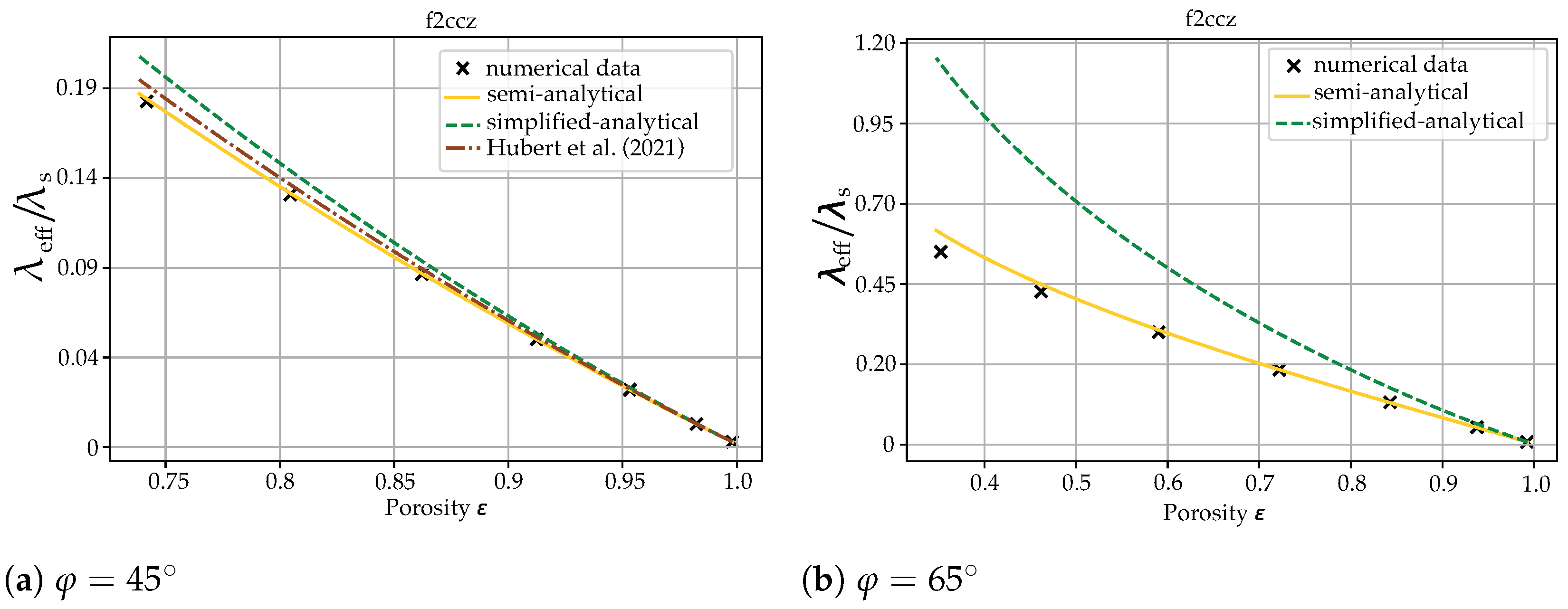
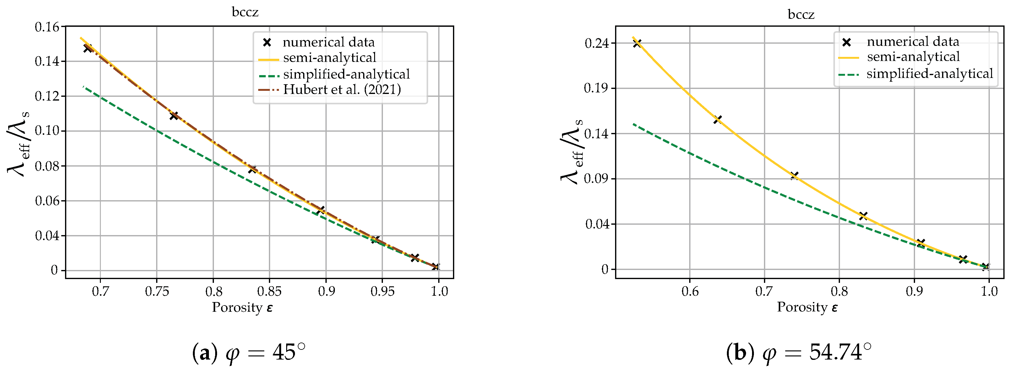
In this work, the effective thermophysical properties of composites based on PCMs embedded with metallic lattice structures are described. Generic geometric parameters are introduced in order to allow the free treatment of all geometric variables and the future topology optimization of such composites. For this purpose, a semi-analytical model for the calculation of the effective thermal conductivity is introduced. The nodes at which the lattice struts cross are described via semi-analytical expressions derived from the use of Steinmetz’s solids. This allows an accurate description of both the porosity of the unit cells and their effective thermal conductivity for a variety of geometric parameters. In the general case, empirical factors must be introduced as analytical solutions for the description of Steinmetz’s solids are limited. Additionally, due to wide manufacturing tolerances, the structures will exhibit non-negligible deviations from the theoretical volume, especially at the nodes where the struts cross. Thus, the empirical factors introduced here can be calibrated in the future depending on the different manufacturing parameters. The model is validated against the existing literature of both previously existing models, which are, however, limited in the number of geometric parameters and experimental results.

A variety of unit cells are considered in a wide range of porosities, i.e., from $ϵ$ = 0.65 to $ϵ$ = 0.99. The main findings of this work are listed below.

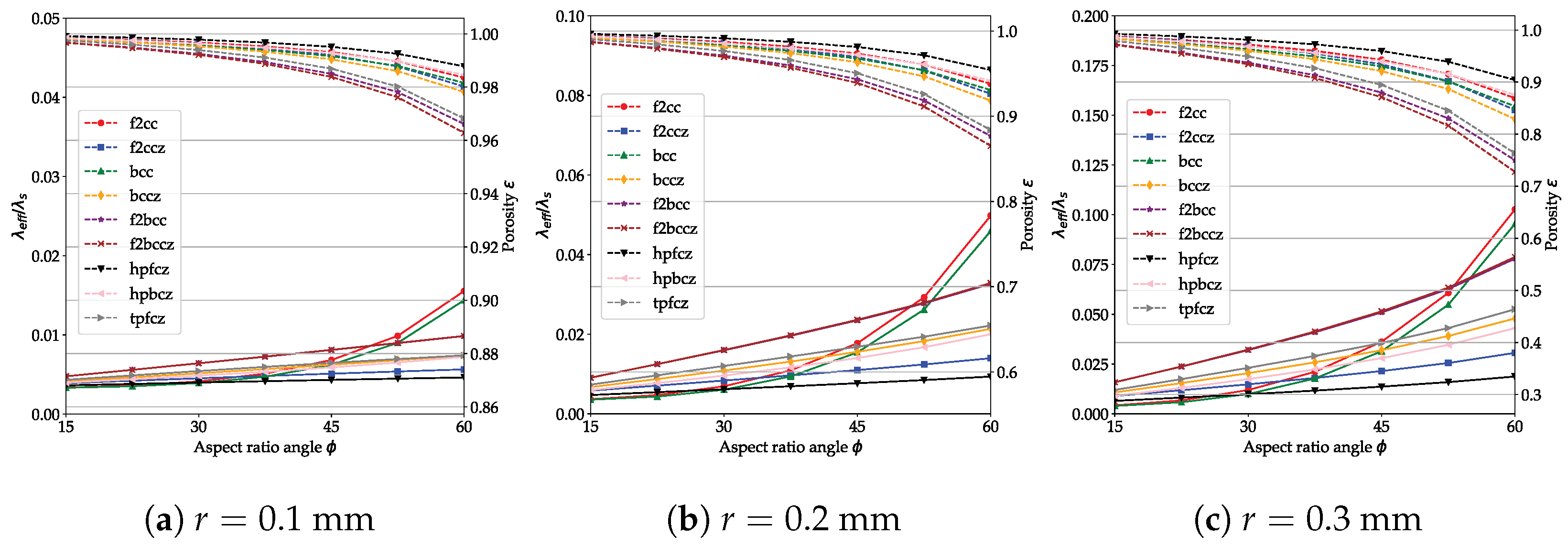
• The cells exhibiting the highest effective thermal conductivity in the 3-direction, i.e., the direction of the z struts, at a given porosity, are the face-centered ones, i.e., $f_{2}cc$,$f_{2}ccz$, $hpfcz$, $tpfcz$.
• In the 1,2-direction, the effective thermal conductivity is obviously reduced for all cells presenting a z strut, and the trends are partially inverted. Body-centered lattices exhibit higher effective thermal conductivity than face-centered ones. Hexagonal cells exhibit the peculiarity of showing the highest and the lowest effective thermal conductivities. The $hpfcz$ consistently shows the highest value in the 3-direction, while the $hpbcz$ exhibits the lowest value. In the 1,2-direction, the trend is reversed and the $hpbcz$ shows the highest effective thermal conductivity.
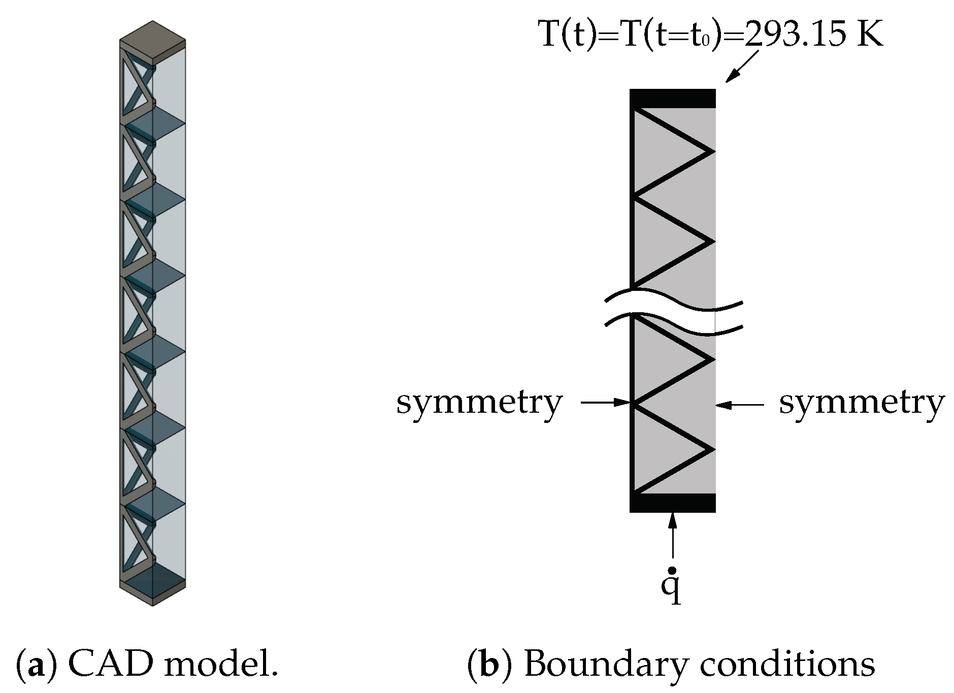
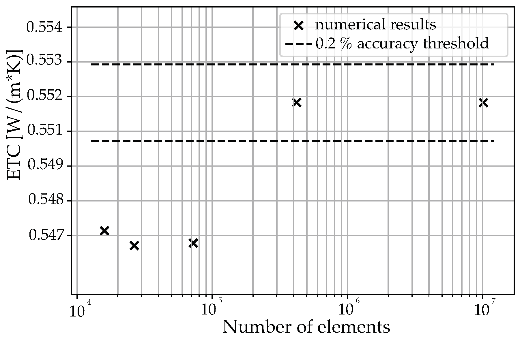
• In general, an increase in the aspect ratio, i.e., increasing the strut angle, leads to higher effective thermal conductivities for unit cells with porosity within ca. 75%.
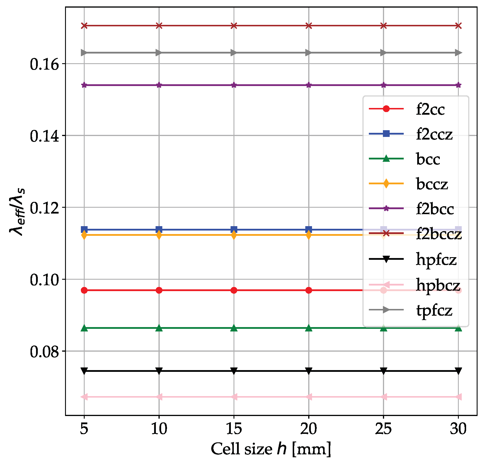
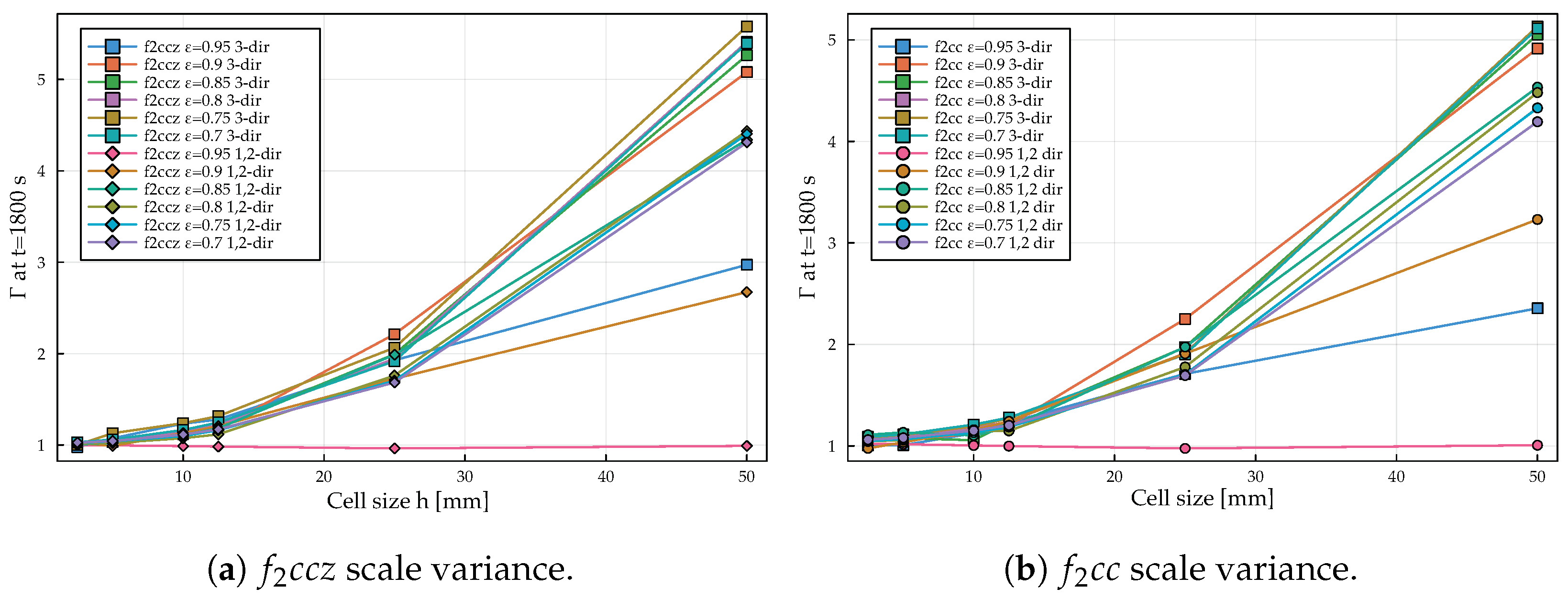
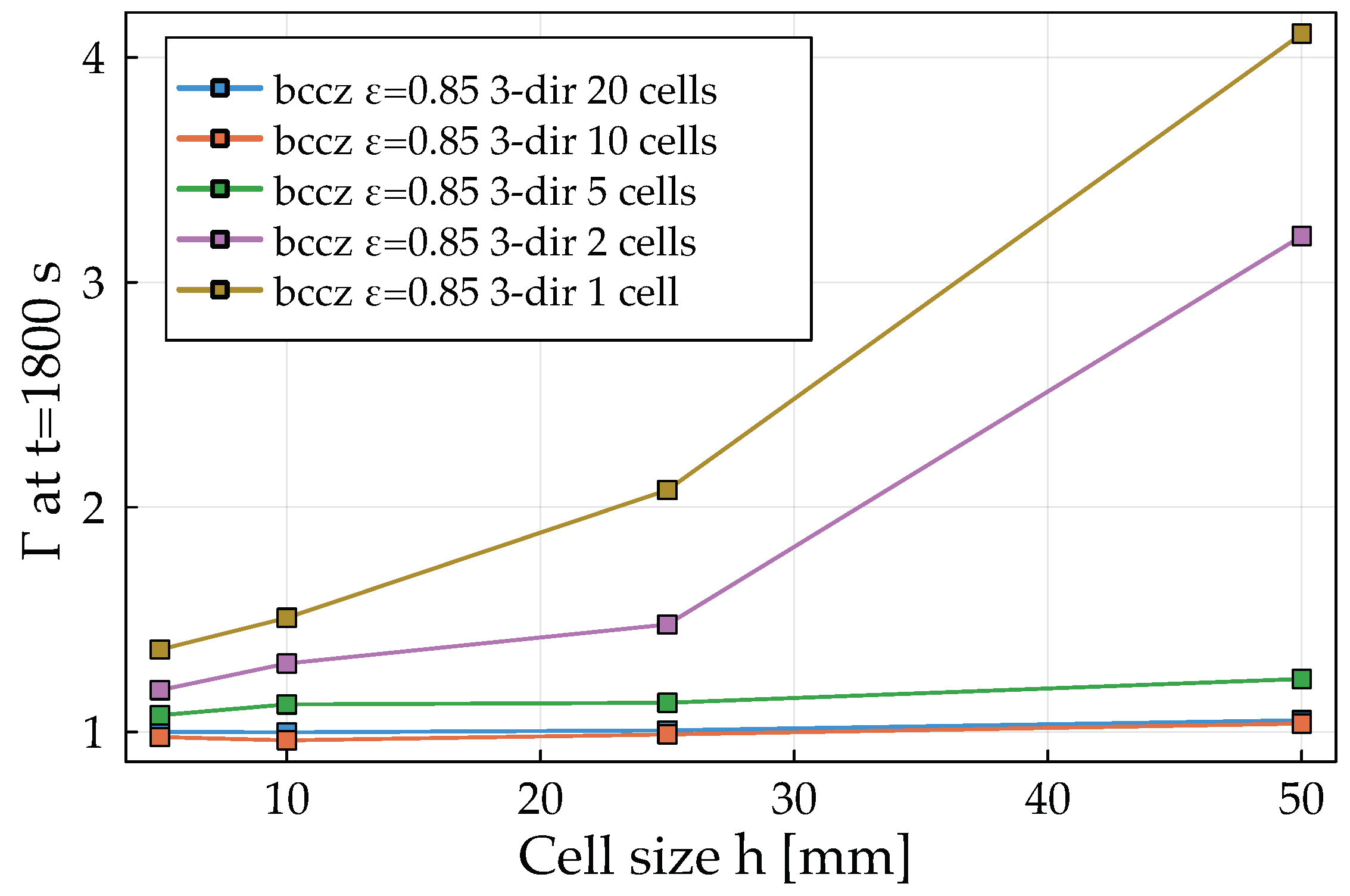
• The effect of the cell size, also called scale variance, indirectly affects the accuracy of the proposed analytical equations. Indeed, if the domain volume is fixed, the variation in the cell size directly influences the number of cells that can fit within such a volume. The number of cells directly affects the transient thermal behavior. A minimum number of cells of 10 is identified as appropriate to describe the transient thermal behavior of the analyzed composites via homogenized models based on effective thermophysical properties. If this threshold is maintained, the cell size has no effect on the transient thermal behavior of the composite. Otherwise, a coupled effect of the reduction in the number of cells and of increasing the cell size can be evidenced. Additionally, the porosity has a direct influence on the scale variance. Indeed, at high porosities, the scale variance, related to the variable $\mathsf{\Gamma }$ of Equation (37), is reduced, while it increases with decreasing porosity.

All in all, the relations delivered in the present work can be flexibly used to estimate the effective thermophysical properties of a variety of composite PCMs. Care should be taken when dealing with a low number of cells and large cell sizes, as homogenization techniques start to fail.

Future works shall address the extension of the presented methodology to additional strut-based cellular solids, in order to extend the comparability of the thermal performance among the different manufacturable geometries. Additionally, prospective activities shall focus on developing methods to perform the same analysis with surface-based lattices, i.e., TPMS. Furthermore, it is well known that natural convection in the melt does have a measurable effect on the speed and shape of the expanding melting front of the PCM, thus affecting the transient thermal performance of the composite. With variable geometric parameters and, in particular, varying the cell size, the influence of natural convection becomes increasingly relevant due to the variation in the permeability of the lattice structure. Future works should extend the presented homogenization approaches to include this additional phenomenon.

References

1. Diaconu, B.M.; Cruceru, M.; Anghelescu, L. Phase Change Materials—Applications and Systems Designs: A Literature Review. Designs 2022, 6, 117. [Google Scholar] [CrossRef]
2. Aramesh, M.; Shabani, B. Metal foam-phase change material composites for thermal energy storage: A review of performance parameters. Renew. Sustain. Energy Rev. 2021, 155, 111919. [Google Scholar] [CrossRef]
3. Gibson, L.J.; Ashby, M.F. Cellular Solids: Structure and Properties, 2nd ed.; Cambridge University Press: Cambridge, UK, 1997. [Google Scholar] [CrossRef]
4. Nazir, A.; Abate, K.M.; Kumar, A.; Jeng, J.Y. A state-of-the-art review on types, design, optimization, and additive manufacturing of cellular structures. Int. J. Adv. Manuf. Technol. 2019, 104, 3489–3510. [Google Scholar] [CrossRef]
5. Yeranee, K.; Rao, Y. A Review of Recent Investigations on Flow and Heat Transfer Enhancement in Cooling Channels Embedded with Triply Periodic Minimal Surfaces (TPMS). Energies 2022, 15, 8994. [Google Scholar] [CrossRef]
6. Righetti, G.; Savio, G.; Meneghello, R.; Doretti, L.; Mancin, S. Experimental study of phase change material (PCM) embedded in 3D periodic structures realized via additive manufacturing. Int. J. Therm. Sci. 2020, 153, 106376. [Google Scholar] [CrossRef]
7. Piacquadio, S.; Schirp-Schoenen, M.; Mameli, M.; Filippeschi, S.; Schröder, K.U. Experimental analysis of the thermal energy storage potential of a phase change material embedded in additively manufactured lattice structures. Appl. Therm. Eng. 2022, 216, 119091. [Google Scholar] [CrossRef]
8. Kaviany, M. Principles of Heat Transfer in Porous Media; Mechanical Engineering Series; Springer: New York, NY, USA, 1995. [Google Scholar] [CrossRef]
9. Ranut, P.; Nobile, E. On the effective thermal conductivity of metal foams. J. Phys. Conf. Ser. 2014, 547, 012021. [Google Scholar] [CrossRef]
10. Calmidi, V.V.; Mahajan, R.L. The Effective Thermal Conductivity of High Porosity Fibrous Metal Foams. J. Heat Transf. 1999, 121, 466–471. [Google Scholar] [CrossRef]
11. Bhattacharya, A.; Calmidi, V.; Mahajan, R. Thermophysical properties of high porosity metal foams. Int. J. Heat Mass Transf. 2002, 45, 1017–1031. [Google Scholar] [CrossRef]
12. Mendes, M.A.; Ray, S.; Trimis, D. A simple and efficient method for the evaluation of effective thermal conductivity of open-cell foam-like structures. Int. J. Heat Mass Transf. 2013, 66, 412–422. [Google Scholar] [CrossRef]
13. Hashin, Z.; Shtrikman, S. A variational approach to the theory of the elastic behaviour of multiphase materials. J. Mech. Phys. Solids 1963, 11, 127–140. [Google Scholar] [CrossRef]
14. Wang, X.; Wei, K.; Wang, K.; Yang, X.; Qu, Z.; Fang, D. Effective thermal conductivity and heat transfer characteristics for a series of lightweight lattice core sandwich panels. Appl. Therm. Eng. 2020, 173, 115205. [Google Scholar] [CrossRef]
15. Kaur, I.; Mahajan, R.L.; Singh, P. Generalized correlation for effective thermal conductivity of high porosity architectured materials and metal foams. Int. J. Heat Mass Transf. 2023, 200, 123512. [Google Scholar] [CrossRef]
16. Gariboldi, E.; Li, Z.; Rawson, A.J. Effective thermal conductivity in BCC and FCC lattices for all volume fractions and conductivity ratios: Analyses by microstructural efficiency and morphology factor and analytic models. Mater. Today Commun. 2022, 33, 104253. [Google Scholar] [CrossRef]
17. Moeini Sedeh, M.; Khodadadi, J. Thermal conductivity improvement of phase change materials/graphite foam composites. Carbon 2013, 60, 117–128. [Google Scholar] [CrossRef]
18. Boomsma, K.; Poulikakos, D. On the effective thermal conductivity of a three-dimensionally structured fluid-saturated metal foam. Int. J. Heat Mass Transf. 2001, 44, 827–836. [Google Scholar] [CrossRef]
19. Dai, Z.; Nawaz, K.; Park, Y.; Bock, J.; Jacobi, A. Correcting and extending the Boomsma–Poulikakos effective thermal conductivity model for three-dimensional, fluid-saturated metal foams. Int. Commun. Heat Mass Transf. 2010, 37, 575–580. [Google Scholar] [CrossRef]
20. Yang, X.H.; Bai, J.X.; Yan, H.B.; Kuang, J.J.; Lu, T.J.; Kim, T. An Analytical Unit Cell Model for the Effective Thermal Conductivity of High Porosity Open-Cell Metal Foams. Transp. Porous Media 2014, 102, 403–426. [Google Scholar] [CrossRef]
21. Yang, H.; Zhao, M.; Gu, Z.; Jin, L.; Chai, J. A further discussion on the effective thermal conductivity of metal foam: An improved model. Int. J. Heat Mass Transf. 2015, 86, 207–211. [Google Scholar] [CrossRef]
22. Hubert, R.; Bou Matar, O.; Foncin, J.; Coquet, P.; Tan, D.; Li, H.; Teo, E.H.T.; Merlet, T.; Pernod, P. An effective thermal conductivity model for architected phase change material enhancer: Theoretical and experimental investigations. Int. J. Heat Mass Transf. 2021, 176, 121364. [Google Scholar] [CrossRef]
23. Angell, I.O.; Moore, M. Symmetrical intersections of cylinders. Acta Crystallogr. Sect. A Found. Crystallogr. 1987, 43, 244–250. [Google Scholar] [CrossRef]
Figure 1. Cubic unit cells. (a) Face-centered cubic,  f 2 c c ; (b) face-centered cubic with z strut,  f 2 c c z ; (c) body-centered cubic,  b c c ; (d) body-centered cubic with z strut,  b c c z ; (e) combined face-centered and body-centered cubic,  f 2 b c c ; (f) combined face-centered and body-centered cubic with z strut,  f 2 b c c z .
Thermo 03 00034 g001
Figure 2. The investigated hexagonal prism unit cells: (a) hexagonal prism with face-centered struts and vertical struts,  h p f c z ; (b) triangular prism with face-centered and vertical struts (i.e., the hexagon is split into triangles, on which the face-centered struts lie),  t p f c z ; (c) hexagonal prism with body-centered and vertical struts,  h p b c z .
Thermo 03 00034 g002
Figure 3. Schematic diagram of the existing effective thermal conductivity models for cellular solids, i.e., foams and lattices. The model presented in this work belongs to the orientation-based layerwise methods.
Thermo 03 00034 g003
Figure 4. Flowcharts introducing the framework of this study and its fundamental steps. (a) Framework of the present study. (b) Detailed description of the framework for the presented model.
Thermo 03 00034 g004
Figure 5. Illustration of the unit cell geometric parameters based on a cell with face-centered struts. The 3-direction corresponds to the z strut direction.
Thermo 03 00034 g005
Figure 6. Steinmetz’s solid for an intersection of two cylinders.
Thermo 03 00034 g006
Figure 7. Workflow to obtain the effective thermal conductivity. (a) Determining the strut types and the quantity of each type, (b) transforming the intersections into cubes and calculating the intersection volumes, (c) modeling the struts in three layers and determining the resistance of each layer, (d) calculating the overall strut resistance using thermal network calculations.
Thermo 03 00034 g007
Figure 8. Transformation of the node intersection into equivalent prismatic volume.
Thermo 03 00034 g008
Figure 9. (a) Two  f 2 c c z  cells stacked in 3-direction; (b) two cells stacked in 1,2-direction.
Thermo 03 00034 g009
Figure 10. Intersection of the struts at the cell corner of the hexagonal cells  h p f c z  and  h p b c z .
Thermo 03 00034 g010
Figure 11. Comparison of the different models for calculation of the porosity of the cell type  f 2 c c . Either the radius r or the angle  φ  is varied. The height of all cells is  h c e l l = 10  mm.
Thermo 03 00034 g011
Figure 13. Convergence study of the stationary model for the  f 2 b c c z  cell, which requires the most elements.
Thermo 03 00034 g013
Figure 14. Comparison of the different models for calculation of the ETC in 3-direction of the cell type  f 2 c c z . The radius is varied between  r = 0.1  mm and  r = 1.3  mm. The height of all cells is  h = 10  mm, while the angle is specified in the caption under the plot. The model for aspect ratio 1 ( φ = 45 ) is validated against the results of Hubert et al. [22]
Thermo 03 00034 g014
Figure 15. Comparison of the different models for calculation of the ETC in 1,2-direction of the cell type  b c c z . The radius is varied between  r = 0.1  mm and  r = 1.3  mm. The height of all cells is  h = 10  mm, while the angle is specified below the plot. The model for aspect ratio 1 ( φ = 45 ) is validated against the results of Hubert et al. [22].
Thermo 03 00034 g015
Figure 16. Example of the overlap of the struts at high angles for the  f 2 c c z  cell. In (a), the cell is shown from an isometric view; in (b), a cross-section cut in the middle vertical plane is shown.
Thermo 03 00034 g016
Figure 17. Comparison of the simulation results based on a homogenized composite and the experimental data from [7].
Thermo 03 00034 g017
Figure 18. Effective thermal conductivity of all considered cells for varying porosity obtained by varying only the strut radius.
Thermo 03 00034 g018
Figure 19. Effect of angle (i.e., aspect ratio) variation for the  f 2 c c z  unit cell at varying porosities, in the 3-direction.
Thermo 03 00034 g019
Figure 20. Effect of varying the aspect ratio angle on the effective thermal conductivity (continuous lines) and on the porosity (dashed lines), respectively, in the 3-direction. Three different radii and thus different porosity ranges are considered. The cell size is fixed at 5 mm.
Thermo 03 00034 g020
Figure 21. Effect of varying the aspect ratio angle on the effective thermal conductivity (continuous lines) and porosity (dashed lines) in the 1,2-direction. Three different radii and thus different porosity ranges are considered. The cell size is fixed at 5 mm.
Thermo 03 00034 g021
Figure 22. Cell size effect on the effective thermal conductivity obtained by scaling the strut radius according to the cell size variation.
Thermo 03 00034 g022
Figure 23. Schematic view of the compared numerical models to investigate the scale variance.
Thermo 03 00034 g023
Figure 24. Scale variance for face-centered cells.
Thermo 03 00034 g024
Figure 25. Scale variance for body-centered cells.
Thermo 03 00034 g025
Figure 26. Isolated effect of varying the number of cells.
Thermo 03 00034 g026